

Abstract
When people try to find particular objects in natural scenes they make extensive use of knowledge about how and where objects tend to appear in a scene. Although many forms of such “top-down” knowledge have been incorporated into saliency map models of visual search, surprisingly, the role of object appearance has been infrequently investigated. Here we present an appearance-based saliency model derived in a Bayesian framework. We compare our approach with both bottom-up saliency algorithms as well as the state-of-the-art Contextual Guidance model of Torralba et al. (2006) at predicting human fixations. Although both top-down approaches use very different types of information, they achieve similar performance; each substantially better than the purely bottom-up models. Our experiments reveal that a simple model of object appearance can predict human fixations quite well, even making the same mistakes as people.
Keywords: Attention, Saliency, Eye movements, Visual search, Natural statistics
The arboreal environments that early primates evolved within demanded keen eyesight to support their ability to find targets of interest (Ravosa & Savakova, 2004; Regan et al., 2001). The ability to visually search for fruits and other foods while avoiding camouflaged predators such as snakes is essential for survival. However, the amount of information in the visual world presents a task too overwhelming for the visual system to fully process concurrently (Tsotsos, 1990). Saccadic eye movements are an overt manifestation of the visual system’s attempt to focus the fovea on important parts of the visual world in a serial manner (Henderson, 1992). In order to accomplish this feat, numerous brain structures, including visual cortex, the frontal eye fields, superior colliculus, the posterior parietal cortex, and the lateral geniculate nucleus (O’Connor, Fukui, Pinsk, & Kastner, 2002) are involved in determining where the next fixation should be directed (Schall, 2002). These brain regions are thought to compute, or influence the computation of, saliency maps, which guide eye movements to regions of interest (Koch & Ullman, 1985; see Itti & Koch, 2001, for a review).
Although the saliency map was originally intended to model covert attention, it has achieved great prominence in models of overt visual attention. In this context, saliency maps attach a value to each location in the visual field given the visual input and the current task, with regions of higher salience being more likely to be fixated. This framework has been extensively used to model eye movements, an overt form of attentional shift. What makes something salient depends on many factors. Generally in the modelling literature it has been assumed a region is salient if it differs greatly from its surroundings (Bruce & Tsotsos, 2006; Gao & Vasconcelos, 2007; Itti, Koch, & Niebur, 1998; Rosenholtz, 1999). Our model, SUN (Saliency Using Natural statistics; Zhang, Tong, & Cottrell, 2007; Zhang, Tong, Marks, Shan, & Cottrell, 2008), defines bottom-up saliency as deviations from the natural statistics learned from experience, and is a form of the kind of “novelty” detector useful in explaining many search asymmetries (see Wolfe, 2001, for a review of the asymmetries).
Recently, the ability of purely bottom-up models to predict human fixations during free viewing has been questioned. It is not clear if bottom-up saliency plays a causal role in human fixation, even if the correlations between predictions and fixations were stronger (Einhäuser & König, 2003; Tatler, 2007; Underwood, Foulsham, van Loon, Humphreys, & Bloyce, 2006). However, it has long been clear that bottom-up models are inadequate for modelling eye movements when top-down task requirements are involved, both intuitively and via some of the earliest studies of eye movements (Buswell, 1935; Einhäuser, Rutishauser, & Koch, 2008; Hayhoe & Ballard, 2005; Yarbus, 1967). For example, when searching for a person in an image, looking for something relatively tall, skinny, and on the ground will provide a more efficient search than hunting for the scene’s intrinsically interesting features.
Several approaches have attempted to guide attention based on knowledge of the task, the visual appearance, or features, of the target. Perhaps the best known is Wolfe’s Guided Search model (1994), which modulates the response of feature primitives based on a number of heuristics. Others have incorporated top-down knowledge into the computation of a saliency map. Gao and Vasconcelos (2005) focus on features that minimize classification error of the class or classes of interest with their Discriminative Saliency model. The Iconic Search model (Rao & Ballard, 1995; Rao, Zelinsky, Hayhoe, & Ballard, 1996; Rao, Zelinsky, Hayhoe, & Ballard, 2002) uses the distance between an image region and a stored template-like representation of feature responses to the known target. Navalpakkam and Itti’s work (2005) finds the appropriate weight of relevant features by maximizing the signal to noise ratio between the target and distractors. Turano, Garuschat, and Baker (2003) combine basic contextual location and appearance information necessary to complete a task, showing vast improvements in the ability to predict eye movements. The Contextual Guidance model (Ehinger, Hidalgo-Sotelo, Torralba, & Oliva, this issue 2009; Oliva, Torralba, Castelhano, & Henderson, 2003; Torralba, Oliva, Castelhano, & Henderson, 2006) uses a holistic representation of the scene (the gist) to guide attention to locations likely to contain the target, combining top-down knowledge of where an object is likely to appear in a particular context with basic bottom-up saliency.
One of the virtues of probabilistic models is that experimenters have absolute control over the types of information the model can use in making its predictions (Geisler & Kersten, 2002; Kersten & Yuille, 2003). As long as the models have sufficient power and training to represent the relevant probability distributions, the models make optimal use of the information they can access. This allows researchers to investigate what information is being used in a biological system, such as the control of human eye fixations.
In this paper we examine two probabilistic models, each using different types of information, that predict fixations made while counting objects in natural scenes. Torralba et al.’s (2006) Contextual Guidance model makes use of global features to guide attention to locations in a scene likely to contain the target. Our model, SUN, contains a top-down component that guides attention to areas of the scene likely to be a target based on appearance alone. By comparing the two approaches, we can gain insight into the efficacy of these two types of knowledge, both clearly used by the visual system, in predicting early eye movements.
THE SUN FRAMEWORK
It is vital for animals to rapidly detect targets of interest, be they predators, food, or targets related to the task at hand. We claim this is one of the goals of visual attention, which allocates computational resources to potential targets for further processing, with the preattentive mechanism actively and rapidly calculating the probability of a target’s presence at each location using the information it has available. We have proposed elsewhere (Zhang et al., 2007, 2008) that this probability is visual saliency.
Let z denote a point in the visual field. In the context of this paper, a point corresponds to a single image pixel, but in other contexts, a point could refer to other things, such as an object (Zhang et al., 2007). We let the binary random variable C denote whether or not a point belongs to a target class,1 let the random variable L denote the location (i.e., the pixel coordinates) of a point, and let the random variable F denote the visual features of a point. Saliency of a point z is then defined as p(C = 1 | F = fz, L = lz) where fz represents the feature values observed at z, and lz represents the location (pixel coordinates) of z. This probability can be calculated using Bayes’ rule:
After making the simplifying assumptions that features and location are independent and conditionally independent given C = 1, this can be rewritten as:
These assumptions can be summarized as entailing that a feature’s distribution across scenes does not change with location, regardless of whether or not it appears on a target.
SUN can be interpreted in an information theoretic way by looking at the log salience, log sz. Since the logarithm is a monotonically increasing function, this does not affect the ranking of salience across locations in an image. For this reason, we take the liberty of using the term saliency to refer both to sz and to log sz, which is given by:
Our first term, −log p(F = fz), depends only on the visual features observed at the point, and is independent of any knowledge we have about the target class. In information theory, −log p(F = fz) is known as the self-information of the random variable F when it takes the value fz. Self-information increases when the probability of a feature decreases—in other words, rarer features are more informative. When not actively searching for a particular target (the free-viewing condition), a person or animal’s attention should be directed to any potential targets in the visual field, despite the features associated with the target class being unknown. Therefore, the log-likelihood and location terms are omitted in the calculation of saliency. Thus, the overall saliency reduces to the self-information term: log sz = −log p(F = fz). This is our definition of bottom-up saliency, which we modelled in earlier work (Zhang et al., 2007, 2008). Using this term alone, we were able to account for many psychological findings and outperform many other saliency models at predicting human fixations while free-viewing.
Our second term, log p(F = fz|C = 1), is a log-likelihood term that favours feature values consistent with our knowledge of the target’s appearance. The fact that target appearance helps guide attention has been reported and used in other models (Rao et al., 1996; Wolfe, 1994). For example, if we know the target is green, then the log-likelihood term will be much larger for a green point than for a blue point. This corresponds to the top-down effect when searching for a known target, consistent with the finding that human eye movement patterns during iconic visual search can be accounted for by a maximum likelihood procedure which computes the most likely location of a target (Rao et al., 2002).
The third term, log p(C = 1|L = lz), is independent of the visual features and reflects any prior knowledge of where the target is likely to appear. It has been shown that if the observer is given a cue of where the target is likely to appear, the observer attends to that location (Posner & Cohen, 1984). Even basic knowledge of the target’s location can be immensely useful in predicting where fixations will occur (Turano et al., 2003).
Now, consider what happens if the location prior is uniform, in which case it can be dropped as a constant term. The combination of the first two terms leads to the pointwise mutual information between features and the presence of a target:
This implies that for known targets the visual system should focus on locations with features having the most mutual information with the target class. This is very useful for detecting objects such as faces and cars (Ullman, Vidal-Naquet, & Sali, 2002). This combination reflects SUN’s predictions about how appearance information should be incorporated into overall saliency, and is the focus of the present paper. SUN states that appearance-driven attention should be directed to combinations of features closely resembling the target but that are rare in the environment. Assuming targets are relatively rare, a common feature is likely caused by any number of nontargets, decreasing the feature’s utility. SUN looks for regions of the image most likely to contain the target, and this is best achieved by maximizing the pointwise mutual information between features and the target class.
In the special case of searching for a single target class, as will be the case in the experiments we are trying to model, p(C = 1) is simply a constant. We can then extract it from the mutual information, thus:
Hence, what we have left can be implemented using any classifier that returns probabilities.
In summary, SUN’s framework is based on calculating the probability of a target at each point in the visual field and leads naturally to a model of saliency with components that correspond to bottom-up saliency, target appearance, and target location. In the free-viewing condition, when there is no specific target, saliency reduces to the self-information of a feature. This implies when one’s attention is directed only by bottom-up saliency, moving one’s eyes to the most salient points in an image can be regarded as maximizing information sampling, which is consistent with the basic assumption of Bruce and Tsotsos (2006). When a particular target is being searched for, as in the current experiments, our model implies the best features to attend to are those having the most pointwise mutual information, which can be modelled by a classifier. Each component of SUN functionally corresponds to probabilities we think the brain is computing. We do not know precisely how the brain implements these calculations, but as a functional model, SUN invites investigators to use the probabilistic algorithm of their choice to test their hypotheses.
EXPERIMENT
When searching for a target in a scene, eye movements are influenced by both the target’s visual appearance and the context, or gist, of the scene (Chun & Jiang, 1998). In either case the pattern of fixations differs significantly compared to when a person is engaged in free-viewing. Although the development of robust models of object appearance is complicated by the number of scales, orientations, nonrigid transformations, and partial occlusions that come into play when viewing objects in the real world, even simple models of object appearance have been more successful than bottom-up approaches in predicting human fixations during a search task (Zelinsky, Zhang, Yu, Chen, & Samaras, 2006). These issues can be evaded to some extent through the use of contextual guidance. Many forms of context can be used to guide gaze ranging from a quick holistic representation of scene content, to correlations of the objects present in an image, to a deeper understanding of a scene.
Here we examine SUN’s appearance-driven model p(C = 1|F = fz), denoted p(C = 1|F) hereafter with other terms abbreviated similarly, and the Contextual Guidance model described by Torralba et al. (2006). Our appearance model leaves out many of the considerations listed previously, but nevertheless it can predict human eye movements in task-driven visual search with a high level of accuracy. The Contextual Guidance model forms a holistic representation of the scene and uses this information to guide attention instead of relying on object appearance.
METHODS
Human data
We used the human data described in Torralba et al. (2006), which is available for public download on Torralba’s website (http://people.csail.mit.edu/torralba/GlobalFeaturesAndAttention/). For completeness, we give a brief description of their experiment. Twenty-four Michigan State University undergraduates were assigned to one of three tasks: Counting people, counting paintings, or counting cups and mugs. In the cup- and painting-counting groups, subjects were shown 36 indoor images (the same for both tasks), and in the people-counting groups, subjects were shown 36 outdoor images. In each of them, targets were either present or absent, with up to six instances of the target appearing in the present condition. Images were shown until the subject responded with an object count or for 10 s, whichever came first. Images were displayed on an NEC Multisync P750 monitor with a refresh rate of 143 Hz and subtended 15.8° × 11.9°. Eye tracking was performed using a Generation 5.5 SRI Dual Purkinje Image Eye tracker with a refresh rate of 1000 Hz, tracking the right eye.
Stimuli used in simulations
The training of top-down components was performed on a subset of the LabelMe dataset (Russell, Torralba, Murphy, & Freeman, 2008), excluding the set used in the human experiments and the data from video sequences. We trained on a set of 329 images with cups/mugs, and 284 with paintings, and 669 with people in street scenes. Testing was performed using the set of stimuli shown to human subjects.
Contextual Guidance model and implementation
Torralba et al. (2006) present their Contextual Guidance model, which is a Bayesian formulation of visual saliency incorporating the top-down influences of global scene context. Their model is
where G represents a scene’s global features, a set of features that captures a holistic representation or gist of an image. F, C, and L are defined as before. Global features are calculated by forming a low dimensional representation of a scene by pooling the low-level features (the same composing F) over large portions of the image and using principal component analysis (PCA) to reduce the dimensionality further. The p(F | G)−1 term is their bottom-up saliency model and the authors approximate this conditional distribution with p(F)−1, using the statistics of the current image (a comparison of this form of bottom-up saliency with SUN’s was performed in (Zhang et al., 2008)). The remaining terms are concerned with top-down influences on attention. The second term, p(F | C = 1, L, G), enhances features of the attended location L that are likely to belong to class in the current global context. The contextual prior term p(L | C = 1, G) provides information about where salient regions are in an image when the task is to find targets from class C. The fourth and final term p(C = 1 | G) indicates the probability of class being present within the scene given its gist. In their implementation both p(F | C = 1, L, G) and p(C = 1 | G) are omitted from the final model. The model that remains is p(C = 1, L | F, G) ≈ p(F)−1 p(L | C = 1, G), which combines the bottom-up saliency term with the contextual priors in order to determine the most salient regions in the image for finding objects of class. To avoid having saliency consistently dominated by one of the two terms, Torralba et al. apply an exponent to the local saliency term: p(C = 1, L | F, G) ≈ p(F)−γ p(L | C = 1, G), where γ is tuned using a validation set.
Our use of Bayes’ rule to derive saliency is reminiscent of the Contextual Guidance model’s approach, which contains components roughly analogous to SUN’s bottom-up, target appearance, and location terms. However, aside from some semantic differences in how overall salience is defined, the conditioning of each component on a coarse description of the scene, the global gist, separates the two models considerably. SUN focuses on the use of natural statistics learned from experience to guide human fixations to areas of the scene having an appearance similar to previously observed instances of the target, whereas the Contextual Guidance model guides attention to locations where the object has been previously observed using the scene’s gist. Although both probabilistic models rely on learning the statistics of the natural world from previous experience, the differences between the formulations affect the meaning of each term, from the source of statistics used in calculating bottom-up saliency to how location information is calculated.
As was done in Torralba et al. (2006), we train the gist model p(L | C = 1, G) on a set formed by randomly cropping each annotated training image 20 times, creating a larger training set with a more uniform distribution of object locations. One difference from Torralba et al. is that we use a nonparametric bottom-up salience model provided to us by Torralba that performs comparably to the original, but is faster to compute. Otherwise, we attempted to be faithful to the model described in Torralba et al. For our data, the optimal γ was 0.20, which is different than what was used in Torralba et al., but is within the range that they found had good performance. Our reimplementation of the Contextual Guidance model performs on par with their reported results; we found no significant differences in the performance measures.
SUN implementation
Recall when looking for a specific target, guidance by target appearance is performed using the sum of the self-information of the features and the log-likelihood of the features given a class. Although we developed efficient ways of estimating the self-information of features in earlier work (Zhang et al., 2008), accurately modelling log p(F | C = 1) or p(F, C = 1) for high dimensional feature spaces and many object classes is difficult. Instead, as described earlier, we extract the log p(C = 1) term (equations repeated here for convenience), which results in a formulation easily implementable as a probabilistic classifier:
The probabilistic classifier we use is a support vector machine (SVM) modified to give probability estimates (Chih-Chung & Chih-Jen, 2001). SVMs were chosen for their generally good performance with relatively low computational requirements. An SVM is simply a neural network with predefined hidden unit features that feed into a particularly well-trained perceptron. The bottom-up saliency term, −log p(F), is still implicitly contained in this model. For the remainder of the paper, we omit the logs for brevity since as a monotonic transform it does not influence saliency.
The first step in our algorithm for p(C = 1 | F) is to learn a series of biologically inspired filters that serve as the algorithm’s features. In SUN’s bottom-up implementation (Zhang et al., 2008), we used two different types of features to model p(F)−1: Difference of Gaussians at multiple scales and filters learned from natural images using independent component analysis (ICA; Bell & Sejnowski, 1995; Hyvärinen & Oja, 1997). Quantitatively, the ICA features were superior, and we use them again here. When ICA is applied to natural images, it yields filters qualitatively resembling those found in visual cortex (Bell & Sejnowski, 1997; Olshausen & Field, 1996). The Fast ICA algorithm2 (Hyvärinen & Oja, 1997) was applied to 11-pixel × 11-pixel colour natural image patches drawn from the Kyoto image dataset (Wachtler, Doi, Lee, & Sejnowski, 2007). This window size is a compromise between the total number of features and the amount of detail captured. We used the standard implementation of Fast ICA with its default parameters. These patches are treated as 363 (11 × 11 × 3) dimensional feature vectors normalized to have zero mean. After all of the patches are extracted, they are whitened using PCA, where each principal component is normalized to unit length. This removes one dimension due to mean subtraction, resulting in 362 ICA filters of size 11 × 11 × 3. When used this way, ICA permits us to learn the statistical structure of the visual world. This approach has been used in biologically inspired models of both face and object recognition (Shan & Cottrell, 2008) and visual attention (Bruce & Tsotsos, 2006; Zhang et al., 2008).
To learn p(C = 1 | F), we find images from the LabelMe dataset (Russell et al., 2008) containing the current class of interest, either people, cups, or paintings. Each image is normalized to have zero mean and unit standard deviation. Using the target masks in the annotation data, d × d × 3 square training patches centred on the object are cropped from the images, with each patch’s size d chosen to ensure the patch contains the entire object. Random square patches of the same size are also collected from the same images, which serve as negative, background examples for C = 0. These came from the same images used to train the Contextual Guidance model. In selecting positive training example patches from the image set, our algorithm ignored objects that consumed over 50% of the training image (permitting negative examples to be taken from the same image) or less than 0.2% of the image (which are too small to extract reliable appearance features). Given the large number of images containing people in street scenes, we chose 800 patches of people randomly from those available. This resulted in 800 patches of people (533 negative examples3), 385 patches of mugs (385 negative examples), and 226 patches of paintings (226 negative examples).
We apply our filters to the set of patches, resizing the filters to each patch’s size to produce one response from each filter per patch. We multiply each response by 112/d2 to make the responses invariant to d’s value and then take the absolute value to obtain its magnitude. The dimensionality of these responses was reduced using PCA to 94 dimensions, a number chosen by cross-validation as explained next.
Three probabilistic SVMs (Chih-Chung & Chih-Jen, 2001) were trained, using the ν-SVC algorithm (Scholkopf, Smola, Williamson, & Bartlett, 2000) with a Gaussian kernel, to discriminate between people/background, paintings/background, and mugs/background. The number of principal components, the same for each SVM, and the kernel and ν parameters for each of the SVMs were chosen using five-fold cross-validation using the training data. The number of principal components was chosen to maximize the combined accuracy of the three classifiers. The kernel and ν parameters of the three SVMs were independently selected for a given number of principal components. We did not tune the classifiers’ parameters to match the human data. Even though our appearance-based features are quite simple, the average cross-validation accuracy across the three classifiers on the training patches was 89%.
Since the scale at which objects appear varies greatly, there is no single optimal scale to use when applying our classifier to novel images. However, objects do tend to appear at certain sizes in the images. Recall that we resized the filters based on the patch size, which was in turn based on the masks people placed on the objects. Hence, we have a scale factor for each training example. Histogramming these showed that there were clusters of scales that differed between the three classes of objects. To take advantage of this information and speed up classification, we clustered the resizing factors by training a one-dimensional Gaussian mixture model (GMM) with three Gaussians using the Expectation-Maximization algorithm (Dempster, Laird, & Rubin, 1977). The cluster centres were initialized using the k-Means+ + algorithm (Arthur & Vassilvitskii, 2007). The three cluster centres found for each class are used to resize the filters when computing p(C = 1 | F). By learning which scales are useful for object recognition, we introduce an adaptive approach to scale invariance, rather than the standard approach of using an image pyramid at multiple octaves. This lets us avoid excessive false positives that could arise in the multiple octave approach. For example, at a very coarse scale, a large filter applied to an image of a person visiting an ancient Greek temple would probably not find the person salient, but might instead find a column that looks person-like.
To calculate p(C = 1 | F), for a test image I, we preprocess the image in the same way as the training images. First, we normalize I to have zero mean and unit variance, then we apply the three scale factors indicated by the cluster centres in the GMM for the object class. For each of our three scales, we enlarge the ICA filter according to the cluster’s mean and normalize appropriately. We convolve each of these filters with the image and take the absolute value of the ICA feature response. These responses are projected onto the previously learned principal components to produce a 94 dimensional feature vector. The SVM for class C provides an estimate of p(C = 1 | F, S = s) for each scale s. This procedure is repeated across the image for all three scales. Each of the maps at scale s is then smoothed using a Gaussian kernel with a half-amplitude spatial width of 1° of visual angle, the same procedure that Torralba et al. (2006) used to smooth their maps in order to approximate the perceptual capabilities of their human subjects. Combining the probability estimates from the three scales at each location is done by averaging the three estimates and smoothing the combined map again using the same Gaussian kernel. This helps ensure the three maps are blended smoothly. Smoothing also provides a local centre of mass, which accounts for the finding that when two targets are in close proximity saccades are made to a point between the two salient targets, putting both in view (Deubel, Wolf, & Hauske, 1984; Findlay, 1983). The same SVM classifier is used for each of the three scales.
RESULTS
In order to compare the ability of SUN’s appearance-based saliency model and the Contextual Guidance model of Torralba et al. (2006) to predict human fixations, we have adopted two different performance measures. Our first measure is the same as used in Torralba et al.: It evaluates the percentage of human fixations being made to the top 20% most salient regions of the saliency map for each subject’s first five fixations. Our second measure of performance is the area under the ROC curve (AUC). It eliminates the arbitrary nature of the 20% threshold evaluation, assessing the entire range of saliency values and revealing the robustness of a particular approach. With this metric, pixels are predicted to be attended or unattended based on whether they are above or below the current saliency threshold; plotting the hit and false alarm rates through all thresholds creates an ROC curve, with the area under the ROC curve being a measure of a model’s ability to predict human fixations (Bruce & Tsotsos, 2006; Tatler, Baddeley, & Gilchrist, 2005). However, the patterns of performance with this second metric remained the same as with the first, so we focus on the first in our discussion (see Figure 3b for AUC data).
Figure 3.

Overall performance in predicting human gaze, across all images and tasks. See the text for a description of the models. (a) Performance assessed by looking at the percentage of fixations falling within the top 20% most salient regions of each image. (b) Performance assessed by looking at the area under the ROC curve. To view this figure in colour, please see the online issue of the Journal.
Due to the tendency of people to fixate near the centre of the screen in free-viewing experiments, it is frequently the case that a Gaussian (or other function decreasing with eccentricity) tuned to the distribution of human fixations will outperform state-of-the-art bottom-up saliency algorithms (Le Meur, Le Callet, & Barba, 2007; Tatler, 2007; Tatler et al., 2005; Zhang et al., 2008). Instead of compensating for these biases as was done in Tatler et al. (2005) and Zhang et al. (2008), we instead assessed whether performance was greater than what could be achieved by merely exploiting them. We examined the performance of a Gaussian fit to all of the human fixations in the test data for each task. Each Gaussian was treated as a saliency map and used to predict the fixations of each subject. Since this includes the current image, this may be a slight overestimate of the actual performance of such a Gaussian. As shown in Figure 3a, there is no significant difference between our implementation of Torralba et al.’s bottom-up saliency and the Gaussian blob, t(107) = 1.391, p = .0835. Furthermore, all methods incorporating top-down knowledge outperformed the static Gaussian, t(107) = 5.149276, p < .00001 for contextual guidance, t(107) = 6.356567, p < .0001 for appearance.
To evaluate how consistent the fixations are among subjects, we determined how well the fixations of seven of the subjects can predict the fixations of the eighth using the procedure of Torralba et al. (2006). This was done by creating a mixture of Gaussians, with a Gaussian of 1° of visual angle placed at each point of fixation for first five fixations from seven of the subjects, to create a map used to predict where the eighth will fixate. We use the same performance measure described earlier. Figures 3 and 4 include these results and Figures 5–8 include subject consistency maps made using this approach.
Figure 4.

Performance of each model by task and condition. The condition refers to whether or not at least one instance of the target was present. The three tasks were counting people, paintings, and cups. The text provides a description for the six models presented. The performance scores indicate what percentage of fixations fell within the top 20 most salient regions for each image. To view this figure in colour, please see the online issue of the Journal.
Figure 5.
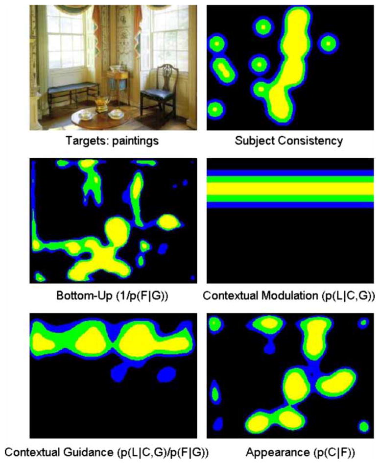
The human fixations and saliency maps produced during a search for paintings. Light grey (yellow), grey (green), and dark grey (blue) correspond to the top 10, 20, and 30% most salient regions respectively. Note that the horizontal guidance provided by contextual guidance is particularly ill-suited to this image, as the attention of both the human subjects and the appearance model is focused on the vertical strip of painting-like wallpaper between the two windows. This figure was selected by identifying images where the Contextual Guidance model and SUN most differed. To view this figure in colour, please see the online issue of the Journal.
Figure 8.
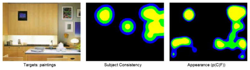
When instructed to find paintings and shown this image, the subjects fixate the television embedded in the cabinet, since it qualitatively looks very much like a painting. SUN makes a similar mistake. To view this figure in colour, please see the online issue of the Journal.
We find appearance provides a better match to the human data, with the overall performance of SUN’s appearance model outperforming the contextual-guidance model when their performance on each task-image pair is compared, t(107) = 2.07, p < .05. Surprisingly, even though the two models of task-based saliency differ considerably in the kind of information they use they both perform similarly overall, with most differences losing statistical significance when a smaller number of images are used in finer levels of analysis (e.g., over tasks or individual fixations).
However, great insight can be gained on the strengths and weaknesses of the two approaches by examining the kinds of saliency maps they produce in greater detail. In order to examine this question, we computed the Euclidean distance between the salience map for each image and task between the Contextual Guidance model, p(L | C, G) p(F | G)−1, and SUN, p(C | F). In Figures 5 and 6, we show two of the maps where the disagreement is large. As can be seen from these images, in these cases, the gist model tends to select single horizontal bands (it is restricted to modelling L along the vertical dimension only) making it difficult to model human fixations that stretch along the vertical dimension, or are bimodal in the vertical dimension. Our appearance model has no such restriction and performs well in these situations. However, these are both limitations of the Contextual Guidance model as implemented, and not necessarily with the concept of contextual guidance itself.
Figure 6.
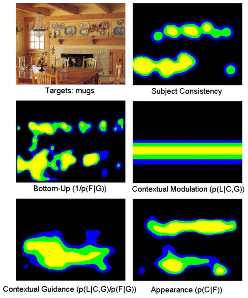
The human fixations and saliency maps produced during a search for cups. Contextual guidance outperformed appearance modelling on this image, although it does not capture the two distinct regions where cups seem most likely two appear. Note than both human subjects and the attention-guidance system are drawn to the cup-like objects above the fireplace. As in Figure 5, light grey (yellow), grey (green), and dark grey (blue) correspond to the top 10, 20, and 30% most salient regions respectively, and this figure was also selected by identifying images where the Contextual Guidance model and SUN most differed. To view this figure in colour, please see the online issue of the Journal.
In Figure 7, we show a case of maximal agreement. Here, the images tend to be “canonical” in that the objects of interest are well-described by a horizontal band, and hence both models can capture the salient regions. Furthermore, most of the interesting textures are confined to a small region of the scene, so even purely bottom-up methods perform comparably.
Figure 7.
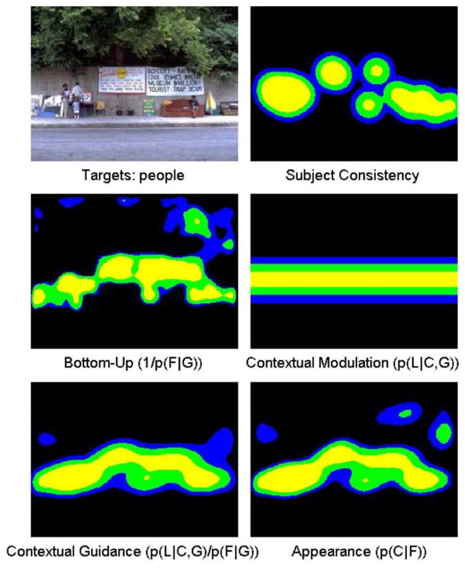
The human fixations and saliency maps produced during a search for people. Here the various models largely agree upon the most salient region of the image. This figure was selected by identifying the image where the Contextual Guidance model and SUN are most similar. As in Figures 5 and 6, light grey (yellow), grey (green), and dark grey (blue) correspond to the top 10, 20, and 30% most salient regions respectively. To view this figure in colour, please see the online issue of the Journal.
The predictions of the Contextual Guidance and our appearance model generally coincide quite well with the human data, but some differences are visually apparent when comparing the maps. This is partially due to thresholding them for display purposes—black regions are not expected to be devoid of fixations, but the models do predict that other regions are more likely to be attended. Additionally, the images in Figures 5 and 6 were chosen as examples where appearance and context differed most, suggesting that these images may be particularly interesting or challenging. However, the subject consistency results in Figures 3 and 4 demonstrate that both models are far from sufficient and must be improved considerably before a complete understanding of fixational eye movements is achieved.
The images in Figures 6 and 8 show the appearance model’s “hallucinations” of potential targets. In Figure 6, there are several objects that might be interpreted as cups and attract gaze during a cup search. In Figure 8, the model confuses the television embedded in the cabinet with a painting, which is the same mistake the subjects make. Torralba et al. (2006) predicted appearance will play a secondary role when the target is small, as is the case here where targets averaged 1° visual angle for people and cups. In support of this prediction, they evaluated the target masks as a salience model, and found the target’s location was not a good indicator of eye fixations. What was missing from this analysis is that an appearance model can capture fixations that would be considered false alarms under the “fixate the target” goal assumed by using the target’s locations. Both our model and the subjects’ visual attention are attracted by objects that appear similar to the target. In this experiment, appearance seemed to play a large role in guiding humans fixations, even during early saccades (we report averages over the first five) and the target absent condition.
We also evaluated how well the task-based models compare to purely bottom-up models. The appearance model of SUN and the Contextual Guidance model both perform significantly better than the Torralba et al. (2006) bottom-up saliency model, t(107) = − 6.440620, p < .0001 for contextual guidance, t(107) = − 7.336285, p < .0001 for appearance. The top-down models also perform significantly better than SUN’s bottom-up saliency model, which was outlined in the Framework section. Since the two bottom-up models perform comparably on this task, t(107) = − 1.240, p = .109, and SUN’s bottom-up component is not of particular interest in the current work, we use the bottom-up component of the Contextual Guidance model in our comparison. See Zhang et al. (2008) for a discussion of how these two models of saliency relate.
Finally, we evaluated how the full SUN model would perform when the location term was included. The LabelMe set provides an object mask indicating the location of each object. We fit a Gaussian with a diagonal covariance matrix to each relevant mask and then averaged the Gaussian responses at each location, after adjusting appropriately to the scale of a given image. The resulting masks provide an estimation of p(L|C). The term p(C|L) is simply p(L|C) × p(C)/p(L), which is constant over an image and does not affect overall salience. We see that its inclusion improves our overall performance significantly, t(107) = 5.105662, p < .0001. We intend to explore these findings further in future work.
DISCUSSION
The experiments we conducted were designed to elucidate the similarities and differences between two models of visual saliency that are both capable of modelling human gaze in a visual search task involving finding and counting targets. Our results support previous findings showing models of bottom-up attention are not sufficient for visual search (Einhäuser et al., 2008; Henderson et al., 2007), and that when top-down knowledge is used, gaze can be better predicted (Torralba et al., 2006; Zelinsky et al., 2006). Although SUN performs significantly better than our reimplementation of the Contextual Guidance model, the differences are small, and both models can assuredly be improved. This coincides well with the results reported by Ehinger et al. (this issue 2009). It is still unclear which plays a larger role when performing visual search in images of real world scenes, appearance or contextual information; presumably, a combination of both could be better than either alone.
We provide computational evidence rejecting the assertion of Torralba et al. (2006) that appearance plays little role in the first few fixations when the target is very small. Their claim was based partly on the limitations of the human visual system to detect small objects, particularly in the periphery. In support of this hypothesis, they found using the labelled regions (e.g., the area labelled “painting”) as the salience model does not completely predict where people look. What their analysis overlooks is that the regions of the image containing targets cannot predict fixations in regions of the image that look like targets. Our coarse features capture the kind of similarity that could be computed by peripheral vision, resulting in the assignment of high salience to regions having an appearance similar to the target object class, allowing an appearance model to predict eye movements accurately even in the target-absent condition. The most recent version of the Contextual Guidance model (Ehinger et al., this issue 2009) incorporates object appearance (their target-feature model), and they find its performance is about the same as bottom-up saliency in the target absent condition using a dataset consisting of pedestrians in outdoor scenes. This may be because they used a sophisticated pedestrian detection algorithm in contrast to our coarse features, but a deeper investigation is needed.
In this work, we did not use the standard image pyramid with scales being separated by octaves, which has been the standard approach for over 20 years (Adelson, Anderson, Bergen, Burt, & Ogden, 1984). However, an image pyramid does not seem appropriate in our model since an object’s representation is encoded as a vector of filter responses. Besides wasting computational resources, using arbitrary scales can also lead to almost meaningless features during classification since the test-input is so different from the input the classifier was trained with. Instead, we learned which scales objects appear at from the training data. Torralba and Sinha (2001) use a similar approach to learn which scales should be used, except their model performs a regression using scene context to select a single scale for a target class. SUN’s scale selection may have been impaired since the distribution of object sizes in the training set is not the same as in the test set, which generally contains smaller objects. However, remedying this by screening the training data would be contrary to the importance we place on learning natural statistics.
Both SUN’s appearance model and the Contextual Guidance model suffer from several noticeable flaws. In both models a separate module is learned for each object class. This is especially a problem for SUN. Humans have the ability to rule out objects after fixating them because they can be identified. Our classifiers are only aware of how the object class they are trained on differs from the background. Hence, when searching for mugs, the mug model has not learned to discriminate paintings from mugs, and so it may produce false alarms on paintings. The use of a single classifier for all classes would remedy this problem; however, current state-of-the-art approaches in machine learning (e.g., SVMs) are not necessarily well suited for learning a large number of object classes. A one-layer neural network with softmax outputs trained on all the classes may be a feasible alternative, as its parameters scale linearly with the number of classes.
In future work, we intend to investigate how different types of top-down (and bottom-up) knowledge can be combined in a principled way. In Torralba et al. (2006), a fixed weighting parameter is used between bottom-up and top-down knowledge, but it seems unlikely that different types of top-down knowledge should be always weighted the same way. If searching for a target with an unreliable appearance but a consistent location, it seems reasonable to weight the location information higher. A method of dynamically selecting the weight depending on the task, visual conditions, and other constraints is likely to significantly improve visual saliency models.
Another important enhancement needed by many saliency models is the explicit incorporation of a retina to model scanpaths in scenes. This has been investigated a few times in models using artificial stimuli (Najemnik & Geisler, 2005; Renninger, Coughlan, Verghese, & Malik, 2005; Renninger, Verghese, & Coughlan, 2007) with each fixation selected to maximize the amount of information gained. Currently SUN produces a static saliency map, with equal knowledge of all parts of the image. Incorporating foveated vision would better model the conditions under which we make eye movements. Likewise, using experiments freed of the monitor would increase the realism of the experimental environment (e.g., Einhäuser et al., 2007); currently our findings are restricted to images displayed on a screen, and it is unclear how well they will generalize.
In conclusion, we have described and evaluated two distinct top-down visual attention models which both excel at modelling task-driven human eye movements, especially compared to solely bottom-up approaches, even though the type of top-down information each uses is considerably different. However, comparing the modelling results with human data it is clear that there is much room for improvement. Integrating appearance, location, and other pieces of top-down information is likely to further improve our ability to predict and understand human eye movements. The probabilistic frameworks we examined are powerful tools in these investigations, allowing investigators to develop models with tightly controlled information access and clearly stated assumptions permitting hypotheses about the information contributing to eye movement control and visual attention to be readily evaluated.
Figure 1.

The three Gaussian mixture model densities learned from the size of the objects in the training data. When searching for a particular object, the cluster centres, indicated by filled circles, are used to select the scales of the ICA filters used to extract features from the image. Note that since the inverse values are clustered a value of 0.1 corresponds to enlarging the original ICA filters to 110 × 110 × 3 while a value of 0.8 only enlarges the filter slightly to 14 × 14 × 3. To view this figure in colour, please see the online issue of the Journal.
Figure 2.
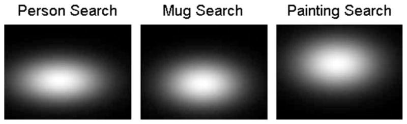
Gaussians fit to the eye movements of subjects viewing these scenes while performing these tasks. Data for eye movements came directly from the test set. By treating these as saliency masks, we can assess the performance of a model that solely makes use of the kinds of eye movements people make performing these tasks.
Acknowledgments
The authors would like to thank Antonio Torralba and his colleagues for sharing their dataset of human fixations, the LabelMe image database and toolbox, and a version of their bottom-up saliency algorithm. We would also like to thank Paul Ruvolo, Matus Telgarsky, and everyone in GURU (Gary’s Unbelievable Research Unit) for their feedback and advice. This work was supported by the NIH (Grant No. MH57075 to GWC), the James S. McDonnell Foundation (Perceptual Expertise Network, I. Gauthier, PI), and the NSF (Grant No. SBE-0542013 to the Temporal Dynamics of Learning Center, GWC, PI and IGERT Grant No. DGE-0333451 to GWC and V. R. de Sa). CK is salso funded by a Eugene Cota-Robles fellowship.
Footnotes
In other contexts, we let C denote the particular class of interest, e.g., people, mugs, or paintings.
Software available at http://www.cis.hut.fi/projects/ica/fastica/
Due to the limited memory capacity of the development machine, the number of background examples for each class was chosen to be at most ⌊800(2/3)⌋ = 533 per object class.
References
- Adelson EH, Anderson CH, Bergen JR, Burt PJ, Ogden JM. Pyramid methods in image processing. RCA Engineer. 1984;29(6):33–41. [Google Scholar]
- Arthur D, Vassilvitskii S. K-means+ +: The advantages of careful seeding. SODA ’07: Proceedings of the eighteenth annual ACM-SIAM symposium on Discrete algorithms; Philadelphia, PA: Society for Industrial and Applied Mathematics; 2007. pp. 1027–1035. [Google Scholar]
- Bell A, Sejnowski T. An information-maximisation approach to blind separation and blind deconvolution. Neural Computation. 1995;7(6):1129–1159. doi: 10.1162/neco.1995.7.6.1129. [DOI] [PubMed] [Google Scholar]
- Bell A, Sejnowski T. The independent components of natural scenes are edge filters. Vision Research. 1997;37(23):3327–3338. doi: 10.1016/s0042-6989(97)00121-1. [DOI] [PMC free article] [PubMed] [Google Scholar]
- Bruce N, Tsotsos J. Saliency based on information maximization. Advances in neural information processing systems. 2006;18:155–162. [Google Scholar]
- Buswell G. How people look at pictures: A study of the psychology of perception in art. Chicago: University of Chicago Press; 1935. [Google Scholar]
- Chih-Chung C, Chih-Jen L. LIBSVM: A library for support vector machines [Computer software] 2001 Retrieved from http://www.csie.ntu.edu.tw/~cjlin/libsvm.
- Chun MM, Jiang Y. Contextual cueing: Implicit learning and memory of visual context guides spatial attention. Cognitive Psychology. 1998;36:28–71. doi: 10.1006/cogp.1998.0681. [DOI] [PubMed] [Google Scholar]
- Dempster A, Laird N, Rubin D. Maximum likelihood from incomplete data via the EM algorithm. Journal of the Royal Statistical Society. 1977;39:1–38. [Google Scholar]
- Deubel H, Wolf W, Hauske G. Theoretical and applied aspects of eye movement research. Amsterdam: North-Holland; 1984. The evaluation of the oculomotor error signal; pp. 55–62. [Google Scholar]
- Ehinger K, Hidalgo-Sotelo B, Torralba A, Oliva A. Modeling search for people in 900 scenes: Close but not there yet. Visual Cognition. 2009;00(00):000–000. doi: 10.1080/13506280902834720. [DOI] [PMC free article] [PubMed] [Google Scholar]
- Einhäuser W, König P. Does luminance-contrast contribute to a saliency map of overt visual attention? European Journal of Neuroscience. 2003;17:1089–1097. doi: 10.1046/j.1460-9568.2003.02508.x. [DOI] [PubMed] [Google Scholar]
- Einhäuser W, Rutishauser U, Koch C. Task-demands can immediately reverse the effects of sensory-driven saliency in complex visual stimuli. Journal of Vision. 2008;8(2):1–19. doi: 10.1167/8.2.2. [DOI] [PubMed] [Google Scholar]
- Einhäuser W, Schumann F, Bardins S, Bartl K, Böning G, Schneider E, König P. Human eye-head co-ordination in natural exploration. Network: Computation in Neural Systems. 2007;18(3):267–297. doi: 10.1080/09548980701671094. [DOI] [PubMed] [Google Scholar]
- Findlay JM. Visual information for saccadic eye movements. In: Hein A, Jeannerod M, editors. Spatially orientated behavior. New York: Springer-Verlag; 1983. pp. 281–303. [Google Scholar]
- Gao D, Vasconcelos N. Discriminant saliency for visual recognition from cluttered scenes. Advances in Neural Information Processing Systems. 2005;17:481–488. [Google Scholar]
- Gao D, Vasconcelos N. Bottom-up saliency is a discriminant process. Paper presented at the IEEE conference on Computer Vision and Pattern Recognition (CVPR); Rio de Janeiro, Brazil. 2007. [Google Scholar]
- Geisler WS, Kersten D. Illusions, perception and Bayes. Nature Neuroscience. 2002;5(6):508–510. doi: 10.1038/nn0602-508. [DOI] [PubMed] [Google Scholar]
- Hayhoe M, Ballard DH. Eye movements in natural behavior. Trends in Cognitive Sciences. 2005;9(4):188–194. doi: 10.1016/j.tics.2005.02.009. [DOI] [PubMed] [Google Scholar]
- Henderson JM. Object identification in context: The visual processing of natural scenes. Canadian Journal of Psychology. 1992;46:319–342. doi: 10.1037/h0084325. [DOI] [PubMed] [Google Scholar]
- Henderson JM, Brockmole JR, Castelhano MS, Mack ML. Visual saliency does not account for eye movements during visual search in real-world scenes. In: van Gompel R, Fischer M, Murray W, Hill R, editors. Eye movements: A window on mind and brain. Oxford, UK: Elsevier; 2007. [Google Scholar]
- Hyvärinen A, Oja E. A fast fixed-point algorithm for independent component analysis. Neural Computation. 1997;9(7):1483–1492. [Google Scholar]
- Itti L, Koch C. Computational modeling of visual attention. Nature Reviews Neuroscience. 2001;3(3):194–203. doi: 10.1038/35058500. [DOI] [PubMed] [Google Scholar]
- Itti L, Koch C, Niebur E. A model of saliency-based visual attention for rapid scene analysis. IEEE Transactions on Pattern Analysis and Machine Intelligence. 1998;20(11):1254–1259. [Google Scholar]
- Kersten D, Yuille A. Bayesian models of object perception. Current Opinion in Neurobiology. 2003;13:1–9. doi: 10.1016/s0959-4388(03)00042-4. [DOI] [PubMed] [Google Scholar]
- Koch C, Ullman S. Shifts in selective visual attention. Human Neurobiology. 1985;4:219–227. [PubMed] [Google Scholar]
- Le Meur O, Le Callet P, Barba D. Predicting visual fixations on video based on low-level visual features. Vision Research. 2007;14(19):2483–2498. doi: 10.1016/j.visres.2007.06.015. [DOI] [PubMed] [Google Scholar]
- Najemnik J, Geisler W. Optimal eye movement strategies in visual search. Nature. 2005;434:387–391. doi: 10.1038/nature03390. [DOI] [PubMed] [Google Scholar]
- Navalpakkam V, Itti L. Modeling the influence of task on attention. Vision Research. 2005;45:205–231. doi: 10.1016/j.visres.2004.07.042. [DOI] [PubMed] [Google Scholar]
- O’Connor DH, Fukui MM, Pinsk MA, Kastner S. Attention modulates responses in the human lateral geniculate nucleus. Nature Neuroscience. 2002;5(11):1203–1209. doi: 10.1038/nn957. [DOI] [PubMed] [Google Scholar]
- Oliva A, Torralba A, Castelhano M, Henderson J. Top-down control of visual attention in object detection. Proceedings of international conference on Image Processing; Barcelona, Catalonia: IEEE Press; 2003. pp. 253–256. [Google Scholar]
- Olshausen BA, Field DJ. Emergence of simple-cell receptive field properties by learning a sparse code for natural images. Nature. 1996;381(6583):607–609. doi: 10.1038/381607a0. [DOI] [PubMed] [Google Scholar]
- Posner MI, Cohen Y. Components of attention. In: Bouma H, Bouwhuis DG, editors. Attention and performance X. Hove, UK: Lawrence Erlbaum Associates Ltd; 1984. pp. 55–66. [Google Scholar]
- Rao R, Ballard D. An active vision architecture based on iconic representations. Artificial Intelligence. 1995;78:461–505. [Google Scholar]
- Rao R, Zelinsky G, Hayhoe M, Ballard D. Modeling saccadic targeting in visual search. Advances in Neural Information Processing Systems. 1996;8:830–836. [Google Scholar]
- Rao R, Zelinsky G, Hayhoe M, Ballard D. Eye movements in iconic visual search. Vision Research. 2002;42(11):1447–1463. doi: 10.1016/s0042-6989(02)00040-8. [DOI] [PubMed] [Google Scholar]
- Ravosa MJ, Savakova DG. Euprimate origins: The eyes have it. Journal of Human Evolution. 2004;46(3):355–362. doi: 10.1016/j.jhevol.2003.12.002. [DOI] [PubMed] [Google Scholar]
- Regan BC, Julliot C, Simmen B, Vienot F, Charlse-Dominique P, Mollon JD. Fruits, foliage and the evolution of primate colour vision. Philosophical Transactions of the Royal Society. 2001;356:229–283. doi: 10.1098/rstb.2000.0773. [DOI] [PMC free article] [PubMed] [Google Scholar]
- Renninger LW, Coughlan J, Verghese P, Malik J. An information maximization model of eye movements. Advances in Neural Information Processing Systems. 2005;17:1121–1128. [PubMed] [Google Scholar]
- Renninger LW, Verghese P, Coughlan J. Where to look next? Eye movements reduce local uncertainty. Journal of Vision. 2007;7(3):1–17. doi: 10.1167/7.3.6. [DOI] [PubMed] [Google Scholar]
- Rosenholtz R. A simple saliency model predicts a number of motion popout phenomena. Vision Research. 1999;39:3157–3163. doi: 10.1016/s0042-6989(99)00077-2. [DOI] [PubMed] [Google Scholar]
- Russell BC, Torralba A, Murphy KP, Freeman WT. LabelMe: A database and web-based tool for image annotation. International Journal of Computer Vision. 2008;77(1–3):157–173. [Google Scholar]
- Schall JD. The neural selection and control of saccades by the frontal eye field. Philosophical Transactions of the Royal Society. 2002;357:1073–1082. doi: 10.1098/rstb.2002.1098. [DOI] [PMC free article] [PubMed] [Google Scholar]
- Scholkopf B, Smola A, Williamson RC, Bartlett PL. New support vector algorithms. Neural Computation. 2000;12:1207–1245. doi: 10.1162/089976600300015565. [DOI] [PubMed] [Google Scholar]
- Shan H, Cottrell G. Looking around the backyard helps to recognize faces and digits. Paper presented at the IEEE conference on Computer Vision and Pattern Recognition (CVPR).2008. [Google Scholar]
- Tatler BW. The central fixation bias in scene viewing: Selecting an optimal viewing position independently of motor biases and image feature distributions. Journal of Vision. 2007;7(14):1–17. doi: 10.1167/7.14.4. Pt. 4. [DOI] [PubMed] [Google Scholar]
- Tatler BW, Baddeley RJ, Gilchrist ID. Visual correlates of fixation selection: Effects of scale and time. Vision Research. 2005;45(5):643–659. doi: 10.1016/j.visres.2004.09.017. [DOI] [PubMed] [Google Scholar]
- Torralba A, Oliva A, Castelhano MS, Henderson JM. Contextual guidance of eye movements and attention in real-world scenes: The role of global features in object search. Psychological Review. 2006;113(4):766–786. doi: 10.1037/0033-295X.113.4.766. [DOI] [PubMed] [Google Scholar]
- Torralba A, Sinha P. Statistical context priming for object detection. Proceedings of the International Conference on Computer Vision; Vancouver, Canada: IEEE Computer Society; 2001. pp. 763–770. [Google Scholar]
- Tsotsos J. Analyzing vision at the complexity level. Behavioral and Brain Sciences. 1990;13(3):423–445. [Google Scholar]
- Turano K, Garuschat D, Baker F. Oculomotor strategies for the direction of gaze tested with a real-world activity. Vision Research. 2003;43:333–346. doi: 10.1016/s0042-6989(02)00498-4. [DOI] [PubMed] [Google Scholar]
- Ullman S, Vidal-Naquet M, Sali E. Visual features of intermediate complexity and their use in classification. Nature Neuroscience. 2002;5(7):682–687. doi: 10.1038/nn870. [DOI] [PubMed] [Google Scholar]
- Underwood G, Foulsham T, van Loon E, Humphreys L, Bloyce J. Eye movements during scene inspection: A test of the saliency map hypothesis. European Journal of Cognitive Psychology. 2006;18:321–343. [Google Scholar]
- Wachtler T, Doi E, Lee T-W, Sejnowski TJ. Cone selectivity derived from the responses of the retinal cone mosaic to natural scenes. Journal of Vision. 2007;7(8):1–14. doi: 10.1167/7.8.6. Pt. 6. [DOI] [PMC free article] [PubMed] [Google Scholar]
- Wolfe JM. Guided Search 2.0: A revised model of visual search. Psychonomic Bulletin and Review. 1994;1:202–228. doi: 10.3758/BF03200774. [DOI] [PubMed] [Google Scholar]
- Wolfe JM. Asymmetries in visual search: An introduction. Perception and Psychophysics. 2001;63(3):381–389. doi: 10.3758/bf03194406. [DOI] [PubMed] [Google Scholar]
- Yarbus AL. Eye movements and vision. New York: Plenum Press; 1967. [Google Scholar]
- Zelinsky G, Zhang W, Yu B, Chen X, Samaras D. The role of top-down and bottom-up processes in guiding eye movements during visual search. Advances in Neural Information Processing Systems. 2006;18:1569–1576. [Google Scholar]
- Zhang L, Tong MH, Cottrell GW. In: McNamara DS, Trafton JG, editors. Information attracts attention: A probabilistic account of the cross-race advantage in visual search; Proceedings of the 29th annual conference of the Cognitive Science Society; Austin, TX: Cognitive Science Society; 2007. pp. 749–754. [Google Scholar]
- Zhang L, Tong MH, Marks TK, Shan H, Cottrell GW. SUN: A Bayesian framework for saliency using natural statistics. Journal of Vision. 2008;8(7):1–20. doi: 10.1167/8.7.32. Pt. 32. Retrieved from http://journalofvision.org/8/7/32/ [DOI] [PMC free article] [PubMed]