Multilevel Latent Class Analysis: An Application of Adolescent Smoking Typologies with Individual and Contextual Predictors

Abstract

Latent Class Analysis (LCA) is a statistical method used to identify subtypes of related cases using a set of categorical and/or continuous observed variables. Traditional LCA assumes that observations are independent. However, multilevel data structures are common in social and behavioral research and alternative strategies are needed. In this paper, a new methodology, multilevel latent class analysis (MLCA), is described and an applied example is presented. Latent classes of cigarette smoking among 10,772 European American females in 9th grade who live in one of 206 rural communities across the U.S. are considered. A parametric and non-parametric approach for estimating a MLCA are presented and both individual and contextual predictors of the smoking typologies are assessed. Both latent class and indicator-specific random effects models are explored. The best model was comprised of three Level 1 latent smoking classes (heavy smokers, moderate smokers, non-smokers), two random effects to account for variation in the probability of Level 1 latent class membership across communities, and a random factor for the indicator-specific Level 2 variances. Several covariates at the individual and contextual level were useful in predicting latent classes of cigarette smoking as well as the individual indicators of the latent class model. This paper will assist researchers in estimating similar models with their own data.

Latent Class Analysis (LCA) is a statistical method used to identify subtypes of related cases using a set of categorical and/or continuous observed variables. These subtypes are referred to as latent classes. The classes are latent in that the subtypes are not directly observed; rather they are inferred from the multiple observed indicators. This method has been used to answer many interesting research questions in the behavioral sciences. For example, recent applications of LCA have assessed alcohol dependence subtypes (Moss, Chen, & Yi, 2007), peer victimization subtypes (Nylund, Bellmore, Nishina, & Graham, 2007), and gambling subtypes (Cunningham-Williams & Hong, 2007).

Traditional LCA assumes that observations are independent of one another. However, in many data structures this assumption is not fulfilled. For example, observations are not independent when the data structure includes students nested in schools, children nested in families, or employees nested in companies. These nested data structures require multilevel techniques. In response to these needs, Vermunt (2003, 2008) and Asparouhov and Muthén (2008) presented a framework for assessing latent class models with nested data.

Consider a Level 1 latent class solution for cigarette smoking typologies that describes three types of smokers: heavy smokers, moderate smokers, and non-smokers. If these individuals were randomly selected from the population, then a traditional, fixed effects latent class analysis would be adequate. However, imagine that these individuals were drawn from 100 different communities across the country. Now, the independence assumption is violated and multilevel latent class analysis is needed.

Multilevel latent class analysis accounts for the nested structure of the data by allowing latent class intercepts to vary across Level 2 units and thereby examining if and how Level 2 units influence the Level 1 latent classes. These random intercepts allow the probability of membership in a particular Level 1 latent class to vary across Level 2 units (e.g., communities). For example, the probability that an individual will belong to the heavy smoking class is likely to vary significantly across communities. That is, in some communities there is a large probability that an individual will belong to the heavy smoker class and in other communities there is a small probability that an individual will belong to the heavy smoker class.

As described by Vermunt (2008) and Muthén and Asparouhov (2009), this multilevel latent class model is akin to a mixed-effects regression model for categorical outcomes (Hedeker, 2003, 2008; Wong & Mason, 1985). However, in the case of multilevel latent class analysis, the dependent variable is latent rather than observed. This latent specification has the added advantage of modeling the measurement error in the observed indicators of the latent class model (Bandeen-Roche, Miglioretti, Zeger, & Rathouz, 1997; Vermunt, 2008).

A new multilevel latent class model is also considered in this paper. This model allows variation across Level 2 units for the intercepts (thresholds) of each latent class indicator. In this way, it is possible to examine how Level 2 units influence the Level 1 indicators that define latent class membership.

In addition to correctly modeling the nested structure of multilevel data, a multilevel latent class analysis allows researchers to assess many interesting research questions. First, in this and any single level latent class analysis, individual (Level 1) covariates may be included in the model. These covariates predict the probability that an individual will belong to a certain Level 1 latent class (e.g., a certain smoking typology). However, multilevel latent class analysis extends the simple assessment of an individual level covariate by permitting the simultaneous assessment of contextual (Level 2) predictors. This feature allows for the possibility that individuals with the same Level 1 covariate values may differ in their probability to belong to a certain latent class (e.g., smoking typology) due to contextual or environmental differences in their community. For example, holding constant important individual level predictors of smoking type, an individual living in a community with a high density of poverty may be more likely to be classified in the heavy smoking latent class than an individual living in a community with a low density of poverty. Consideration and assessment of contextual level predictors in the framework of a latent class analysis has implications for many salient research questions in the social and behavioral sciences.

In this paper, latent classes of cigarette smoking among 10,772 European American adolescent females in 9th grade who live in one of 206 different rural communities across the contiguous U.S. is considered. This data structure represents a nested or multilevel design in which individuals represent Level 1 of the hierarchy and communities represent Level 2. We demonstrate two techniques for assessing a multilevel latent class analysis, a parametric and a non-parametric approach, and we also consider both individual and contextual level predictors of the smoking typologies. Student level predictors include age, attachment to school, school performance, educational aspirations, parental school expectations, parental involvement in school, friends' fondness for school, and association with friends who have dropped out of school. Community level predictors include proportion of minors in the community who live in poverty, total population of the community, and a binary variable to indicate whether or not each community is located in one of the tobacco growing states.

Random effects in a latent class model

A traditional, multilevel analysis for a binary outcome may be estimated using a logistic regression model. In an unconditional model the probability of the outcome (e.g., being a smoker vs. a non-smoker) is constant within each Level 2 unit; that is, in each Level 2 unit there is some probability of being a smoker. A random coefficient model considers the Level 2 units to be drawn from a population of Level 2 units, and the probability of the outcome (i.e., being a smoker) across groups is considered to be a random variable (Snijders & Bosker, 2002).

Thus, for an observed binary outcome C_ij, where i denotes the individual and j denotes the Level 2 unit, a logit link function is applied in a two-level logistic regression model. We define P_ij as the probability that C_ij = 1, and the log odds of P_ij, logit(P_ij), as the natural log of P_ij / (1- P_ij). The two-level logistic random intercept regression model can then be expressed as:

$$\mathit{\text{logit}}(P_{\mathit{\text{ij}}})={\beta }_{\mathit{0}j}+{\beta }_{\mathit{1}}{x}_{\mathit{\text{ij}}}(\text{Level}1)$$ (1)

$${\beta }_{\mathit{0}j}={\gamma }_{\mathit{0}}+{\gamma }_{\mathit{1}}{w}_j+U_{\mathit{0}j}.(\text{Level}2)$$ (2)

This implies that P_ij can be expressed as the logistic function:

$$P_{\mathit{\text{ij}}}=\frac{\text{exp}({\gamma }_0+{\beta }_1{x}_{\mathit{\text{ij}}}+{\gamma }_1{w}_j+U_{0j})}{1+\text{exp}({\gamma }_0+{\beta }_1{x}_{\mathit{\text{ij}}}+{\gamma }_1{w}_j+U_{0j})}.$$ (3)

Equations (1) and (2) show that the logit, or log odds, is formulated as a random intercept model, where β_0j is the random intercept. At Level 2, the log odds of the outcome for a particular Level 2 unit j is defined as the population average of the log odds (γ₀ + γ₁ w_j) plus the random deviation from this average for the group (U_0j). These random deviations are assumed to be normally distributed. The magnitude of the U₀ variance indicates the strength of the influence of the Level 2 units. That is, a larger variance indicates greater influence of the Level 2 units. As shown in equations 1 and 2, this model easily incorporates predictors at Level 1 (i.e., x_ij) and Level 2 (i.e., w_j). For example, one may use variables such as age, gender, or race as Level 1 predictors of the log-odds of smoking and variables such as unemployment rate or poverty rate of communities as Level 2 predictors of the Level 2 random intercept.

This same framework may be used to consider random effects within a latent class analysis. Here, an observed C_ij is replaced with a latent C_ij. First consider the case of two latent classes (e.g., a smoker latent class and a non-smoker latent class), where individuals (Level 1) are nested in communities (Level 2). In this case, let C_ij represent the latent classes variable. Here, we assess the log-odds of belonging to the smoker class rather than the non-smoker class and we allow the log-odds to vary across communities. That is, we specify one random intercept to capture this variability in the log-odds. For example, in some communities the log-odds of being a smoker are quite high, in other communities the log-odds of being a smoker are quite low. We assume that the variance in log-odds is normally distributed across Level 2 units.

If the Level 1 latent class model (i.e., smoking typologies) is best defined by more than two latent classes, a two-level multinomial logistic regression is used. Here, T-1 random intercepts are specified, where T equals the number of Level 1 latent classes. For example, consider three, Level 1 latent classes: heavy smokers, moderate smokers, and non-smokers. If we select non-smokers as the reference group, we then need to specify two random intercepts. One represents the variability in the log-odds of membership in the heavy smoker class across communities and one represents the variability in the log-odds of membership in the moderate smoker class across communities. Essentially this allows the probability that an individual will belong to a particular Level 1 latent class to vary across Level 2 units. This method of specifying a multilevel latent class analysis represents the parametric approach to multilevel latent class analysis proposed by Vermunt (2003, 2008) and Asparouhov and Muthén (2008).

As is the case in any latent class model, the latent class variable is defined by multiple observed indicators. This latent specification has the advantage of modeling the measurement error in the observed indicators of the latent class model (Bandeen-Roche, Miglioretti, Zeger, & Rathouz, 1997; Vermunt, 2008) and the indicators together contribute to better capture the true smoking status of the individual. For simplicity and in line with Vermunt (2003), random intercepts are typically not included for the latent class indicators, but it is assumed that cluster effects are sufficiently well represented by the latent class random effects (this assumption will be relaxed in the next section). Considering the case where the latent class indicators are binary indicators (U_ijk), the model may be written as follows for K indicators:

$$P(U_{\mathit{\text{ij}}1}=s_1,U_{\mathit{\text{ij}}2}=s_2,\dots U_{\mathit{\text{ijK}}}=s_K)=\sum _{t=1}^{T}P(C_{\mathit{\text{ij}}}=t)\prod _{k=1}^{K}P(U_{\mathit{\text{ijk}}}=s_k|C_{\mathit{\text{ij}}}=t)$$ (4)

where U_ijk represents the response of individual i in Level 2 unit j on indicator k and s_k is the specific response for the k^th indicator. The latent class variable denoting latent class membership is defined by C_ij, a specific latent class is referred to as t, and the total number of latent classes by T. The probability of a specific response pattern, P(U_ij=s), is the weighted average of the probabilities conditional on class membership. Using equation (3), the weight, P(C_ij=t),is the probability that person i in Level 2 unit j is a member of latent class t,

$$P(C_{\mathit{\text{ij}}}=t)=\frac{\text{exp}({\gamma }_0+{\beta }_1{x}_{\mathit{\text{ij}}}+{\gamma }_1{w}_j+U_{0j})}{1+\text{exp}({\gamma }_0+{\beta }_1{x}_{\mathit{\text{ij}}}+{\gamma }_1{w}_j+U_{0j})}$$ (5)

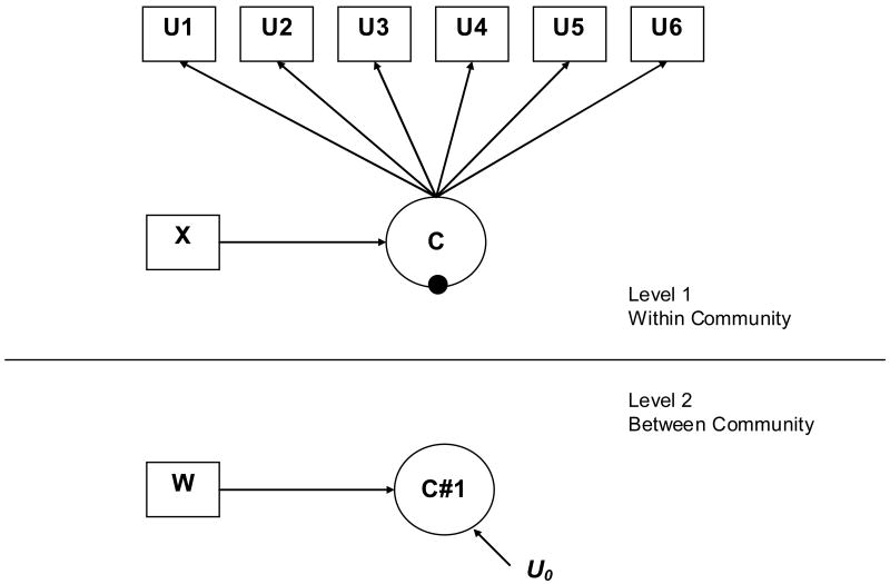
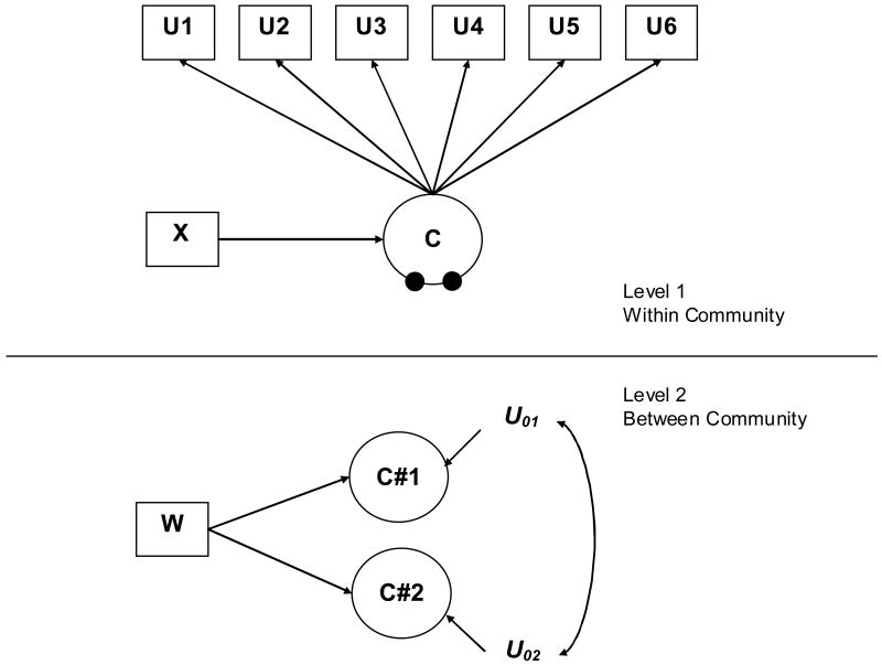
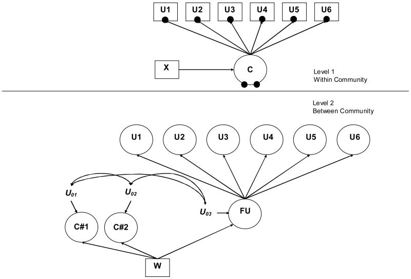
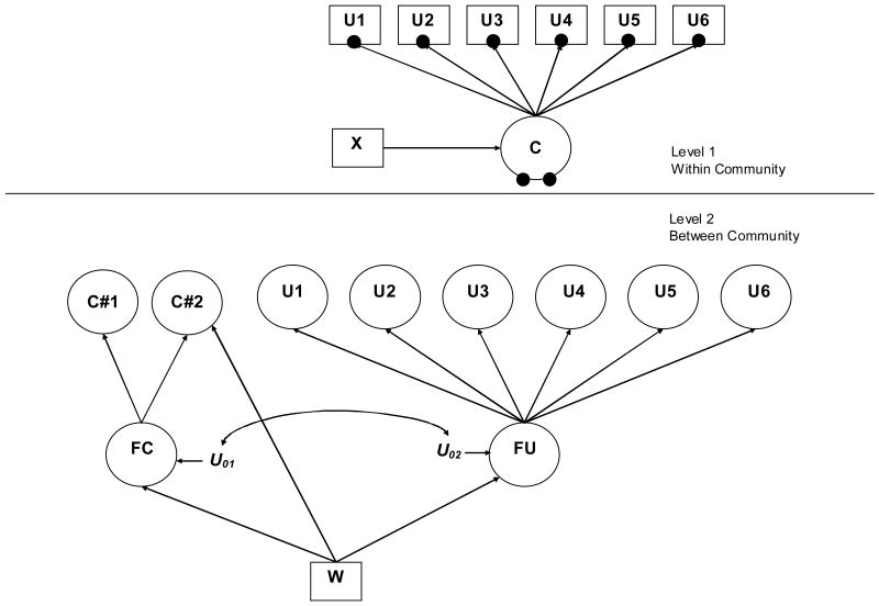
Figure 1 presents an example of a parametric multilevel latent class model where individuals are nested in communities. In this example there are two within-community (Level 1) latent classes (C). In the within-community model the single filled circle represents the random mean for the within-community latent classes (there are T-1 random means, where T equals the number of Level 1 latent classes). This random mean is referred to as C#1 in the between communities model. It is a continuous latent variable that varies across communities. In the parametric approach, the mean(s) from the Level 1 latent class solution is allowed to vary across communities. In the case of three or more latent classes, the T-1 random means are correlated with one another (see Figure 2 for a model with 3 latent classes).

Figure 1.

Multilevel Latent Class Model with Two Level 1 Latent Classes—Parametric Approach

Figure 2.

Multilevel Latent Class Model with Three Level 1 Latent Classes—Parametric Approach

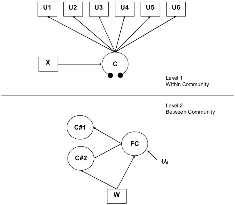
As discussed by Vermunt (2003) and Van Horn and colleagues (2008), this model can be computationally heavy, particularly as Level 1 latent classes increase. Following work by Bock (1972) and Hedeker (1999), Vermunt (2003) and Asparouhov and Muthén (2008) recommends the use of a common factor to model the random means and associated covariances. This model operates under the assumption that the random means are highly correlated, and these random means may be best represented by a single factor where different random means have different factor loadings. Specifying zero residual variances, this factor model reduces the dimensionality of the random means from T-1 to 1. This simplification avoids heavy computations due to numerical integration in the maximum-likelihood estimation. Whether or not this common factor model for the Level 2 random means provides a better fit than the fully random model described above is an empirical question. If a reasonable fit is obtained, this specification can drastically reduce computation time. This model is shown in Figure 3 for three classes (T=3).

Figure 3.

Multilevel Latent Class Model with Three Level 1 Latent Classes—Parametric Approach with Level 2 Factor on Random Latent Class Intercepts

Vermunt (2003, 2008) and Asparouhov and Muthén (2008) also proposed a non-parametric approach to multilevel latent class analysis. In this approach a second latent class model is specified at Level 2. The T -1 random means from the Level 1 latent class solution are used as indicators of a second latent class model at Level 2. The different Level 2 latent classes have different distributions of the random means; that is, the log-odds of membership in a particular Level 1 latent class. In this approach, the normal distribution that is assumed of the random means in the parametric approach is replaced with the assumption of a multinomial distribution (Vermunt, 2008). Essentially, this means that a normal distribution is replaced by a discrete distribution in the form of a histogram, where non-normality is allowed. As a result, the non-parametric approach avoids the assumption of normality and is less computationally demanding (Muthén & Asparouhov, 2008).

The resultant Level 2 latent classes describe differences in the probability of membership in each Level 1 latent class. The result is a finite number of Level 2 latent classes that capture the Level 2 variability in the distribution of Level 1 latent class membership probabilities. As such, Level 2 units that are similar with regard to the distribution of individual level typologies are grouped together and defined as separate from Level 2 units with a different distribution of individual level typologies. For example, using the 3-class, Level 1 smoking typology example (i.e., heavy smokers, moderate smokers, and non-smokers), the Level 2 latent class solution may be defined by two latent classes: one that represents communities where individuals have a high probability of being a non-smoker and one that represents communities where individuals have a high probability of being a heavy or moderate smoker.

In the nonparametric approach, the equation for the Level 1 latent class solution is defined as follows:

$$P(C_{\mathit{\text{ij}}}=t|C{B}_j=m)=\frac{\text{exp}({\gamma }_{\mathit{\text{tm}}})}{\text{∑}_{r=1}^T\text{exp}({\gamma }_{\mathit{\text{rm}}})},$$ (6)

where CB_j represents group j's score on the latent class variable that defines the discrete mixture distribution and m represents a specific mixture.

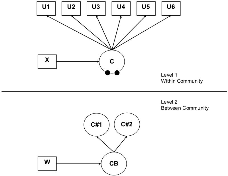
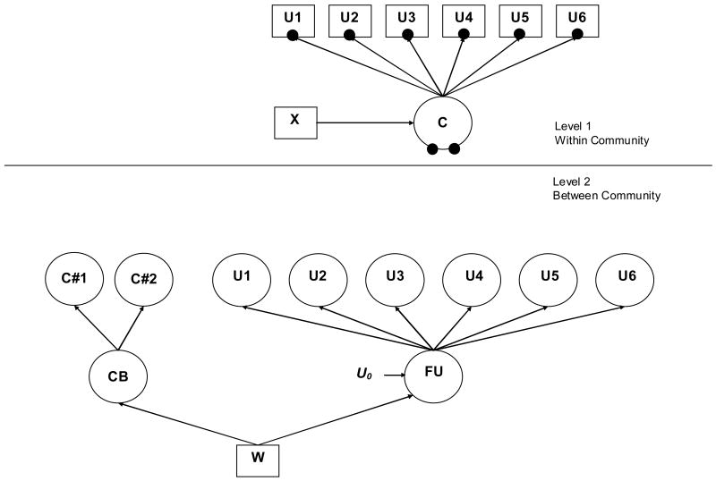
Figure 4 presents an example of the non-parametric approach to multilevel latent class analysis. In the non-parametric approach, the specification of the random means is different than in the parametric approach. As described by Bijmolt, Paas and Vermunt (2004), these random means vary across the Level 2, between communities latent classes (labeled CB in the figure). This variation of Level 1 parameters across Level 2 units is the key feature of any multilevel model, and in a multilevel latent class analysis it is this variation that defines the between-community latent classes. Specifically, the Level 2 (i.e., community level) latent classes are defined by the random means from the Level 1 latent class solution.

Figure 4.

Multilevel Latent Class Model with Three Level 1 Latent Classes—Non-Parametric Approach

Indicator-specific random effects

Although not discussed in the current literature, additional random effects based on the individual indicators that define the Level 1 latent class model may be specified within the framework of Asparouhov and Muthén (2008). Here, the conditional item probabilities of (4) are extended to have random intercepts (thresholds in Mplus):

$$\mathit{\text{logit P}}(U_{\mathit{\text{ijk}}}=S_k|C_{\mathit{\text{it}}}=t)={\tau }_{\mathit{\text{jkt}}},$$ (7)

with j varying over Level 2 units, k denoting the indicators, and t denoting the latent class. To reduce dimensionality between groups (i.e., Level 2) a common factor is defined by the indicator intercepts τ_jkt. This factor varies over the Level 2 units labeled j and captures indicator-specific cluster influence using different factor loadings for different random intercepts. Specifying zero residual variances, this factor model reduces the dimensionality of the random intercepts from 6 to 1. This simplification avoids heavy computations due to numerical integration in the maximum-likelihood estimation. This specification may provide a better fit to the data and also allows for the assessment of how Level 2 units may influence the individual indicators that define the Level 1 latent class model. This technique may be used in both the parametric and non-parametric approaches described above. Figures 5 and 6 present this model for the parametric approach (without and then with the Level 2 factor on the random intercepts respectively). Figure 7 presents this approach for the nonparametric approach.

Figure 5.

Multilevel Latent Class Model with Three Level 1 Latent Classes—Parametric Approach with Level 2 Factor on Random Latent Class Indicators

Figure 6.

Multilevel Latent Class Model with Three Level 1 Latent Classes—Parametric Approach with Level 2 Factor on Random Latent Class Intercepts and Level 2 Factor on Random Latent Class Indicators

Figure 7.

Multilevel Latent Class Model with Three Level 1 Latent Classes—Non-Parametric Approach with Level 2 Factor on Random Latent Class Indicators

Addition of covariates

Once a multilevel latent class structure is specified, covariates may be introduced at both level l and Level 2. For the parametric approach, Level 1 covariates predict membership in a certain Level 1 latent class. These analyses are carried out using multinomial logistic regression. In addition, Level 2 covariates may be specified to predict the T-1 random means. These analyses are carried out using linear regression. Level 2 covariates predict a community's probability that an individual will belong to a certain Level 1 latent class.

For the non-parametric approach, Level 1 latent classes can be predicted by Level 1 and Level 2 covariates (in the same fashion as the parametric approach) and Level 2 latent classes can be predicted by Level 2 covariates. In this case, a Level 2 covariate (poverty rate of the community) predicts the probability that a community will belong to a Level 2 latent class defined by a high probability of heavy smoking. In the non-parametric approach, covariate effects at both levels are tested using multinomial logistic regression.

Inclusion of a common factor on the Level 1 latent class indicators also permits assessment of Level 2 covariates on the individual indicators making up the Level 1 latent class model. For example, a Level 2 covariate may affect membership in a certain Level 1 latent class, but also an individual indicator of the latent class model.

Methods

Sample

Participants in this study are 10,772 European-American, female, 9th grade students from 206 communities in the contiguous United States who participated in a national study of substance use in rural communities between 1996 and 2000. We restrict the sample to European-American 9^th grade girls in order to simplify the example; however, assessment of this same model for girls of other ethnic backgrounds and boys is an important future step. The sample was constructed to, as closely as possible, yield a stratified, representative, sample of rural schools in the contiguous U.S. Details about the study design may be found in Stanley, Comello, Edwards and Marquart (2008).

Within each community, surveys were administered at a single public high school and the public feeder junior-high/middle school(s). In the relatively small percentage of cases where there was more than one high school in the community, the high school determined to be the most representative socio-demographically of the community and its feeder schools were chosen.

Procedure

Students were given the Community Drug and Alcohol Survey (CDAS)¹. The CDAS is a 99-item survey that asks a variety of questions related to substance use; school adjustment; relationships with family and peers; and other individual risk factors for substance use. The CDAS is a variation of the American Drug and Alcohol Survey (Oetting, Edwards, & Beauvais, 1985) which has been in use since the mid-1980s. Its measures have been through rigorous reliability and validity analysis (Oetting & Beauvais, 1990-1991), and it is one of the instruments listed in SAMHSA's Measures and Instruments Resource guide (SAMHSA, 2007). Surveys were given with passive parental consent, and procedures ensured complete confidentiality. Across schools, the percent of students surveyed ranged from 75-100% of the total student body.

Measures

Six categorical indicators were used to inform latent class membership. Lifetime incidence of cigarette smoking (1=yes, 0=no), current smoking status (0=non-smoker, 1=smokes “once in a while,” and 2=smokes everyday), self-identification as a smoker (0=non-smoker, 1=light smoker, and 2=moderate to heavy smoker), friend's smoking status (0= most friends don't smoke, 1=most friends smoke), perception that parents would try to stop them from smoking (1=yes, 0=no), and perception that regular cigarette smoking is harmful to one's health (1=yes, 0=no).

At Level 1, the student level, several predictors of the Level 1 latent class membership were considered: age (all students were in 9th grade, but age did significantly vary) and several school-related protective factors in the individual, family, and peer domain. In the individual domain, we considered measures of school bonding, performance at school, and academic aspirations. The school bonding scale included four items, each measured on a 4-point scale, where a higher score indicated better bonding. Items included measures of fondness for school, perception that school was fun, fondness for teachers, and perception that teachers liked the student (coefficient alpha=.84). The school performance scale included two items, each measured on a 4-point scale ranging from “poor” to “very good”: What kind of grades do you get?, What kind of student are you? Coefficient alpha=.86. The aspirations scale used two items to assess students' perceptions that they would graduate from high school and go to college. Each item was measured on a five-point scale ranging from “No chance that I will,” to “Yes, I'm sure that I will.” Coefficient alpha=.73. In the family domain, we considered a measure of the student's perception of their parent's concern about their academic achievement/behavior at school. The scale included four items: How much would your family care if you…skipped school, got a bad grade, did not do your homework, quit school. All items were measured on a four point scale ranging from “not at all” to “a lot.” Coefficient alpha=.73. We also considered parental involvement in school, measured with two items: Does your family go to school events?, Does your family go to school meetings (PTA, PTO, back to school nights, etc.)? Both items were measured on a 4-point scale ranging from “no” to “a lot.” Coefficient alpha=.64. Finally, in the peer domain, we considered a measure of friend's fondness for school and association with friends who have dropped out of school. Friends fondness for school consisted of a three-item scale (friend's like school, think school is fun, and like their teachers). All three items were measured on a 4-point scale ranging from “not at all” to “a lot.” Coefficient alpha=.87. Association with friends who dropped out of school was a dichotomous item (1=yes, 0=no).

At Level 2, the community level, several predictors were considered, including proportion of individuals in the community under the age of 17 who were living in poverty at the 2000 census, the natural log of the total population in the community at the 2000 census, and a binary variable to indicate if the community resided in a tobacco-growing state (1=yes, 0=no).

All models were estimated in Mplus Version 5.2 (Muthén & Muthén, 1998-2008) using a maximum likelihood estimator with robust standard errors.

Results

A traditional LCA of the six smoking indicators was first examined. These initial analyses ignored the clustering of students in communities. Table 1 presents the class solutions for one to six latent classes (see Model 1). The BIC drastically declines (i.e., improves) from 1 to 3 classes and then begins to level off. Entropy is also best with the 3-class model. Moreover, the 4-class solution separates one of the classes from the 3-class solution into two smaller groups, but the posterior probabilities indicates that there is substantial misclassification between these two smaller classes. For example, the posterior probabilities for the 3-class solution are .99, .93, .98 and the posterior probabilities for the 4-class solution are .79, .93, .98, and .79, with the first and fourth classes representing the separated classes from the 3-class model. The low posterior probabilities for these two classes indicate that the model has difficulty distinguishing between people in the first and fourth class. Most importantly, the substantive interpretation of the 3-class solution (as described in the next section) is theoretically meaningful, useful, and parsimonious. As such, we chose the 3-class solution as the best model. The results are presented in Table 2.

TABLE 1. Fit Criteria for Each Model Specification.

Model	Number of Level 1 Classes
	1 Class	2 Classes	3 Classes	4 Classes	5 Classes	6 Classes
1. Fixed effects model
No. of free parameters	8	17	26	35	44	53
Log-likelihood	−41,813	−31,013	−29,204	−29,090	−29,057	−29,040
BIC	83,700	62,185	58,650	58,505	58,523	58,572
Lo–Mendell–Rubin LRT	N/A	21,343	3,575	226	65	34
Entropy	1.00	0.98	0.96	0.76	0.73	0.73
2. Random effects model, parametric
No. of free parameters		18	29	41
Log-likelihood		−30,769	−28,902	−28,694
BIC		61,705	58,074	57,768
Entropy		0.98	0.96	0.77
3. Random effects model, parametric with factor on the Level 2 random intercepts
No. of free parameters		N/A	28	38
Log-likelihood			−28,916	−28,713
BIC			58,093	57,779
Entropy			0.96	0.77
4. Random effects model, nonparametric
4a. 2 between classes
No. of free parameters		19	29	39
Log-likelihood		−30,825	−28,984	−28,800
BIC		61,827	58,236	57,961
Entropy		0.91	0.92	0.81
4b. 3 between classes
No. of free parameters		21	32	43
Log-likelihood		−30,792	−28,944	−28,746
BIC		61,778	58,185	57,892
Entropy		0.91	0.90	0.79
5. Random effects model, parametric with factor on Level 1 latent class indicators
No. of free parameters		25	37	a
Log-likelihood		−30,422	−28,737
BIC		61,076	57,817
Entropy		0.98	0.96
6. Random effects model, parametric with factor on Level 1 latent class indicators and factor on Level 2 random intercepts
No. of free parameters		N/A	35	45
Log-likelihood			−28,751	−28,652
BIC			57,827	57,722
Entropy			0.96	0.75
7. Random effects model, nonparametric with factor on Level 1 latent class indicators
7a. 2 between classes
No. of free parameters		26	36	46
Log-likelihood		−30,482	−28,833	−28,728
BIC		61,206	58,000	57,883
Entropy		0.91	0.92	0.87
7b. 3 between classes
No. of free parameters		29	40	51
Log-likelihood		−30,447	−28,785	−28,687
BIC		61,162	57,942	57,848
Entropy		0.91	0.91	0.88

Note. BIC = Bayesian information criterion; LRT = likelihood ratio test;

^aModel is too computationally intensive to estimate.

N/A = not applicable

TABLE 2. Latent Class Solution for Three-Class Model (No Level 2 Model).

Indicator	Class 1 14.6% Heavy Smoker	Class 2 24.1% Moderate Smoker	Class 3 61.3% Nonsmoker
	Ever smoked a cigarette
	No	0.00	0.00	0.78
Yes	1.00	1.00	0.22
Current smoking status
Does not smoke	0.00	0.04	1.00
Smokes once in a while	0.11	0.94	0.00
Smokes every day	0.89	0.02	0.00
Self-identification as a smoker
Nonsmoker	0.03	0.16	1.00
Light smoker	0.06	0.79	0.00
Moderate to heavy smoker	0.92	0.05	0.00
Most friends smoke
No	0.10	0.44	0.83
Yes	0.90	0.56	0.17
Parents would stop subject from smoking
No	0.30	0.08	0.04
Yes	0.70	0.93	0.97
Perceives smoking harms health
No	0.40	0.23	0.14
Yes	0.60	0.77	0.86

In this 3-class solution, the largest class represents non-smokers and comprises 61.3% of the sample. While some of these students had smoked a cigarette in their lifetime, none of them were current smokers or thought of themselves as a smoker. Moreover, they tended to associate with non-smoking peers, believe that their parents would stop them from smoking, and perceive that smoking is harmful. The smallest class, described as the heavy smokers, represents 14.6% of the sample. Girls in this class tended to be regular smokers and viewed themselves as a heavier smoker. They also tended to associate mostly with other peers who smoked cigarettes and were less likely than other girls to perceive that their parents would stop them from smoking and that smoking is harmful. The remaining students were classified as moderate or occasional cigarette smokers. Comprising 24.1% of the sample, these students were most likely to report occasional cigarette smoking and viewed themselves as light smokers. Just over half of them reported that most of their friends smoke. Nearly all believed that their parents would try to stop them from smoking and about three-quarters believed that smoking is harmful to one's health.

Building on this 3-class, Level 1 solution, we next specified a model that utilized the parametric approach to account for the nested structure of the data. The results of the model are presented in Table 1, Model 2. The BIC improves with the addition of the random effects and the entropy remains the same as for the fixed effects model. The estimated mean of the random effect (or random mean) for the heavy smoker class indicates that, for communities at the average random mean for both heavy smoking and moderate smoking, the average probability that a student would be classified as a heavy smoker is .13. The variance of the random mean describes the variation in the probability that a student will belong to the heavy smoking class across communities (i.e., in some communities the probability is quite high, in others it is quite low). This variance is statistically significant, V(U_0j)=.61, se=.10, and indicates that communities did indeed vary significantly in their probability that a female would be a heavy smoker. Specifically, holding the probability of membership in the moderate smoker class constant, the probability that a female is a heavy smoker in a community that is 1 standard deviation below the mean of the random mean is .06 and 1 standard deviation above the mean of the random mean is .25. Larsen and Merlo (2005) offer an alternative measure to quantify the between community variation, the Median Odds Ratio (MOR). The MOR is an estimate of the difference in the probability of the outcome for two randomly chosen people from two different randomly chosen Level 2 units. The MOR between a student in a community with the higher propensity to be a heavy smoker and a student with a lower propensity to be a heavy smoker is 2.10. This is a moderate odds ratio and also indicates substantial community-level variability in the probability of heavy smoking.

The estimated mean of the random effect (or random mean) for the moderate smoker class indicates that, for communities at the average random mean for both heavy smoking and moderate smoking, the average probability that a student would be classified as a moderate smoker is .26. The variance of this random mean describes the variation in the probability that a student would be classified as a moderate smoker across communities. This variance is also statistically significant, V(U_0j)=.23, se=.05. Holding the probability of membership in the heavy smoker class constant, the probability that a female is a moderate smoker in a community that is 1 standard deviation below the mean of the random mean is .17 and 1 standard deviation above the mean of the random mean is .38. The MOR is 1.57. This is a small odds ratio, and indicates that there is some variability across communities in the probability of being a moderate smoker, but considerable less than for heavy smoking.

We also estimated the neighboring two and four class parametric random effects models. With the addition of the random effects, the three class model still appears to be the best model. The BIC shows a large decline from two classes to three, and a much smaller decline from three classes to four. Moreover, entropy is maximized with three classes and the fourth class produced in the 4-class solution is not well distinguished from one of the other classes. It should be noted that more research is needed to understand the performance of BIC in multilevel latent class models.

We extended this model by including a common factor on the Level 2 random means for the 3-class and 4-class solutions (Model 3). This dramatically reduced computation time and resulted in a reasonably small increase in BIC. The substantive interpretation of the Level 1 latent class solutions remained the same, including the qualitative typologies defined by each class and the proportion of individuals in each class.

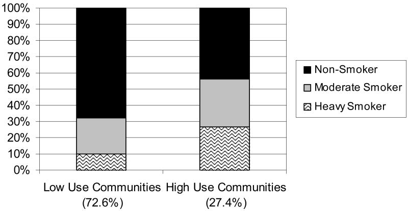
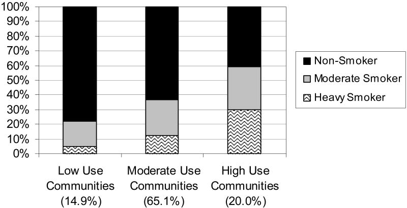
In the next set of models we utilized the non-parametric approach. In this case, a Level 2 latent class model was added based on the random means from the Level 1 latent class solution. As presented in Table 1 (Model 4a), the BIC significantly improves over the fixed effects 3-class model with the addition of two, Level 2 latent class; however, the BIC is not better than the BIC for the parametric model. Adding a third class only slightly improves the BIC, but it still does not show improvement over the parametric approach. A fourth Level 2 class was also assessed, but this model resulted in a very small number of individuals in the fourth class and the best log-likelihood failed to replicate. The results of the Level 2 latent class solution for the CB=2 and CB=3 solutions are presented in Figures 8 and 9.

Figure 8.

Non-Parametric Multilevel Latent Class Solution, C=3, CB=2

Figure 9.

Non-Parametric Multilevel Latent Class Solution, C=3, CB=3

With two Level 2 latent classes (Figure 8 – Model 4a in Table 1), one Level 2 latent class is comprised of communities with a relatively large number of non-smokers (i.e., 68% of the females are non-smokers). This class represents nearly 73% of the students. The second Level 2 latent class is comprised of communities with more heavy and moderate smokers. This class represents about 27% of students.

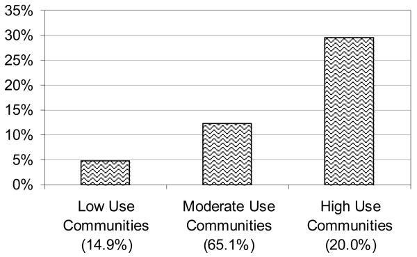
With three Level 2 latent classes (Figure 9 – Model 4b in Table 1), a low use community, moderate use community, and heavy use community emerges. Most students lived in one of the moderate use communities (65%), in these communities, about 64% of the females were non-smokers. Figure 10 demonstrates the nonparametric characterization of the random logit means. Here, the distribution of the random means is not assumed or represented to be normal, as is the case in the parametric ML LCA model. Rather, the histogram captures the discrete distribution of the random means. For example, in Figure 10, the random mean distribution for the Level 1 heavy smoker class is represented by three bars showing a skewed distribution across the Level 2 latent classes.

Figure 10.

The Discretized, Non-Normal Distribution of the Non-Parametric Approach. The bars represent the percent of students in the heavy user class in each between communities latent class from the C=3, CB=3 solution.

We also estimated the neighboring Level 1 two and four class nonparametric random effects models. The model with three Level 1 classes appears to be superior, showing a substantial decline over the model with two Level 1 classes, maintaining a high entropy value, and providing the most substantively interesting solution.

As a final step, we examined the inclusion of a common Level 2 factor for the individual indicators making up the Level 1 latent class model. For both the parametric (Models 5 and 6) and non-parametric approach (Model 7a and 7b), these models represented a marked improvement in log-likelihood and BIC. For example, when comparing Model 3 (the parametric model with Level 2 factor for random means) to Model 6 (the parametric model with Level 2 factor for random means and a factor for the Level 1 latent class indicators) for the 3-class solution, BIC improves from 58093 to 57827, with a difference of seven parameters. Similar improvements are observed for the non-parametric approach (Model set 4 compared to Model set 7). These improvements indicate that communities have a substantial influence on the Level 1 indicators of individual smoking typologies.

Synthesizing the information from all three multilevel models presented in Table 1, we find that the parametric approach with the inclusion of a common factor on the latent class indicators provides the best BIC for these data. Moreover, adding a second common factor on the Level 2 random means greatly decreases computation time and complexity, with minimal increase in BIC. As such, we selected this 3-class parametric random effects model with a factor on the latent class indicators and a factor on the Level 2 random means (Model 6) for further examination. We extended this model by including predictors at Level 1 (i.e., individual characteristics) and Level 2 (community characteristics). This was accomplished by regressing latent class membership on the Level 1 predictors via a multinomial logistic regression, and regressing both the random means and the latent class indicators on the Level 2 predictors via linear regression. Because of the common factor for the Level 2 random means and the common factor for the Level 1 latent class indicators, the Level 2 covariate effects must be carefully specified and interpreted. The sum of the indirect and direct effect of a particular covariate onto a random intercept C# is calculated as follows using the example of the covariate effect when comparing Class 2 to Class 3. The Class 2 factor loading λ₂ is multiplied by the coefficient γ for the regression of the common factor on the covariate, and the direct effect γ₂ of the covariate on the random intercept is added – that is, λ₂*γ+γ₂. For C#1 λ = 1 and since C#1 is identical to the common factor, the regression coefficient for the common factor regressed on the covariate is the total effect. Table 3 presents the results of these conditional models.

TABLE 3. Results of the Conditional Multilevel Latent Class Analysis: Effects on Level 1 Latent Class Solution.

	Comparison of Moderate Smoker to Non-Smoker			Comparison of Heavy Smoker to Non-Smoker
	Odds	95% Cl		Odds	95% Cl
		−	+		−	+
Level 1 Predictors
Age	1.03	0.95	1.13	1.37	1.21	1.55
School bonding	0.87	0.80	0.94	0.74	0.66	0.84
School performance	0.67	0.63	0.71	0.54	0.49	0.59
Academic aspirations	0.94	0.88	1.01	0.81	0.75	0.88
Parent's school expectations	0.90	0.85	0.96	0.82	0.75	0.89
Parental involvement at school	0.85	0.80	0.91	0.69	0.63	0.77
Friend's school bonding	0.94	0.88	1.00	0.81	0.72	0.90
Friends have dropped out of school	2.38	2.10	2.69	6.29	5.08	7.79
Level 2 Predictors
Log of total population	1.03	0.96	1.10	1.01	0.89	1.14
Tobacco growing state	1.02	0.82	1.27	1.39	1.00	1.94
Proportion of youth living in poverty	7.00	2.48	19.74	2.40	0.45	12.75

At Level 1, latent class membership was regressed on the student level predictors in a multinomial logistic regression. In this model, the non-smoker latent class served as the reference group. The first set of columns in Table 3 presents the results that compare the moderate smokers to the non-smokers. The odds that a girl would be a moderate smoker (compared to a non-smoker) were significantly higher as her school bonding decreased, school performance decreased, parent's expectations for academic achievement decreased, parent's involvement in school decreased, involvement with friend's who were well bonded to school decreased (although this is a marginally significant effect), and if she associated with friends who had dropped out of school As is the case in any regression model, the effect of each covariate represents its unique effect after adjusting for all other variables in the model. School bonding, school performance, parental expectations for academic achievement, parental involvement in school, and friend's school bonding were all standardized to a mean of 0 and a standard deviation of one. Therefore we can interpret the regression coefficients as follows: for each one standard deviation increase in school bonding, the odds of being a moderate smoker as compared to a non-smoker decreased by about 13%, with similar interpretations for all other continuous school-related covariates. Since involvement with friends who dropped out of school is binary, the odds ratio indicates that the odds of being a moderate smoker as compared to a non-smoker were about 2.4 times higher if a girl associated with friends who had dropped out of school.

The second set of columns in Table 3 presents the results that compare the heavy smokers to the non-smokers. The odds that a girl would be a heavy smoker (compared to a non-smoker) were significantly higher if she were older, as her school bonding decreased, school performance decreased, academic aspirations decreased, parent's expectations for academic achievement decreased, parent's involvement in school decreased, involvement with friend's who were well bonded to school decreased, and if she associated with friends who had dropped out of school. While all covariates are robust predictors of heavy smoking, involvement with friends who had dropped out of school is particularly strong. The odds of being a heavy smoker were 6.3 times higher if a girl associated with high school dropouts.

At Level 2, the random means from the Level 1 LCA were regressed on three community level predictors. The non-smoker class was used as the reference group in this model as well. When comparing moderate smokers to non-smokers, we find that proportion of youth living in poverty is the only significant predictor. This indicates that, holding all other predictors constant, as the proportion of young people living in poverty in the community increased, more girls indicated moderate smoking as compared to no smoking. When comparing heavy smokers to non-smokers we find that living in a tobacco growing state is the only significant predictor (p=.05). Communities in a tobacco growing state had more girls who were heavy smokers than non-smokers. Specifically, the odds of being a heavy smoker is 39% higher if the community is located in a tobacco growing state.

Finally, several Level 2 covariate effects on the Level 1 latent class indicators were observed. These results are reported in Table 4. Tobacco growing state had an effect on friend's smoking, in that the probability of endorsing the friend's smoke indicator was higher if the respondent lived in a tobacco growing state. Level of poverty in the community affected several of the latent class indicators. Poverty was significantly associated with all indicators except parental sanctions against smoking.

TABLE 4. Results of the Conditional Multilevel Latent Class Analysis: Effects on Level 1 Latent Class Indicator Intercepts.

	Level 2 Predictor
	Log of Total Population			Tobacco-Growing State			Proportion of Youth Living in Poverty
	Odds	95% Cl		Odds	95% Cl		Odds	95% Cl
		−	+		−	+		−	+
Ever smoked a cigarette	1.03	0.97	1.09	1.16	0.98	1.38	3.95	1.51	10.29
Current smoking status	1.03	0.97	1.10	1.18	0.97	1.43	4.40	1.27	15.31
Self-identification as a smoker	1.02	0.98	1.05	1.09	0.97	1.22	2.22	1.12	4.41
Most friends are smokers	1.04	0.97	1.12	1.26	1.01	1.56	7.78	2.83	21.40
Parent's would stop subject from smoking	0.99	0.97	1.01	0.95	0.88	1.02	0.63	0.37	1.09
Perceives smoking harms health	0.99	0.97	1.01	0.94	0.88	1.01	0.59	0.38	0.92

Discussion

In this paper we presented an applied example of a multilevel latent class analysis. The example assessed smoking typologies among rural-dwelling, European-American adolescent girls. At Level 1, three latent classes emerged: heavy smokers, moderate smokers, and non-smokers.

We accounted for the nesting of students in communities using two models to incorporate random effects for the latent class variable – a parametric approach and a non-parametric approach. In our example the parametric approach provided the best fit to the data. This model allowed the probability that a girl would belong to the heavy smoker class or the moderate smoker class to vary across communities. This properly accounted for the fact that in some communities the probability that a girl was a heavy smoker or a moderate smoker was quite high, while in other communities these same probabilities were quite low. We also found that improved fit was obtained by adding a common factor to the Level 1 latent class indicators, and allowing this common factor to vary across communities. This allowed for estimation of cluster level influences. Finally, by adding a second common factor on the Level 2 random means, we were able to achieve a model that was vastly easier to estimate from a computation perspective. This model resulted in only a slightly higher BIC and the substantive interpretation remained the same.

We extended the parametric random effects unconditional model to examine the effect of several Level 1 and Level 2 predictors. At Level 1, the results indicate that smoking typologies may be predicted by age, level of school bonding, school performance, academic aspirations, parental expectations for academic achievement, parental involvement in school, friends' school bonding, and association with friends who dropped out of school. At Level 2, the results indicate that communities with more minors living in poverty had more adolescent girls who were moderate smokers and communities located in a tobacco growing state had more adolescent girls who were heavy smokers.

Over the past several decades many substantively interesting questions in the social and behavioral sciences have been addressed using latent class analysis. This paper describes the technique by which latent class models may be utilized when data are hierarchical, a commonly encountered data structure. Multilevel latent class analysis is useful for properly modeling the nested structure of the data, but also allows researchers to answer interesting substantive questions about contextual, upper level predictors.

Given the emphasis in social and behavioral research to adopt an ecological systems approach to understanding human behavior (Bronfenbrenner, 1986), this relatively new method to assess latent class typologies in contextual studies should allow for the assessment of many important studies that concern contextual level predictors of individual typologies of behavior. This paper makes a significant contribution to the literature by presenting the multilevel latent class model in a manner that is accessible to applied researchers, providing an applied example, and presenting the syntax to estimate each model.

Mplus Syntax for Specified Models

3-class fixed effects model (Model 1 in Table 1)

• MISSING IS.;

• USEVARIABLES = EVSMK SMK30TRI HEAVY FRSMK PARSTOP TOBHARM;

• CLASSES=C(3);

• CATEGORICAL ARE EVSMK SMK30TRI HEAVY FRSMK PARSTOP TOBHARM;

• ANALYSIS: TYPE = MIXTURE;

• STARTS = 60 30;

• PROCESS=8(STARTS);

3-class random effects model – parametric approach (Model 2 in Table 1)

• MISSING IS.;

• USEVARIABLES = EVSMK SMK30TRI HEAVY FRSMK PARSTOP TOBHARM;

• CLASSES=C(3);

• CATEGORICAL ARE EVSMK SMK30TRI HEAVY FRSMK PARSTOP TOBHARM;

• CLUSTER=LEAID;

• WITHIN=EVSMK SMK30TRI HEAVY FRSMK PARSTOP TOBHARM;

• ANALYSIS: TYPE = MIXTURE TWOLEVEL;

• STARTS = 20 10;

• PROCESS=8(STARTS);

• MODEL:

• %WITHIN%

• %OVERALL%

• %BETWEEN%

• %OVERALL%

• C#1; C#2; C#1 WITH C#2;

3-classes at Level 1, 2-classes at Level 2 random effects model – non-parametric approach (Model 4a in Table 1)

• MISSING IS.;

• USEVARIABLES = EVSMK SMK30TRI HEAVY FRSMK PARSTOP TOBHARM;

• CLASSES=CB(2) CW(3);

• CATEGORICAL ARE EVSMK SMK30TRI HEAVY FRSMK TOBHARM PARSTOP;

• CLUSTER=LEAID;

• BETWEEN=CB;

• WITHIN=EVSMK SMK30TRI HEAVY FRSMK TOBHARM PARSTOP;

• ANALYSIS: TYPE = MIXTURE TWOLEVEL;

• STARTS = 20 10;

• PROCESS=8(STARTS);

• MODEL:

• %WITHIN%

• %OVERALL%

• %BETWEEN%

• %OVERALL%

• CW ON CB;

• MODEL CW:

• %WITHIN%

• %CW#1%

• [EVSMK$1 SMK30TRI$1 SMK30TRI$2 HEAVY$1 HEAVY$2 FRSMK$1 TOBHARM$1 PARSTOP$1];

• %CW#2%

• [EVSMK$1 SMK30TRI$1 SMK30TRI$2 HEAVY$1 HEAVY$2 FRSMK$1 TOBHARM$1 PARSTOP$1];

• %CW#3%

• [EVSMK$1 SMK30TRI$1 SMK30TRI$2 HEAVY$1 HEAVY$2 FRSMK$1 TOBHARM$1 PARSTOP$1];

3-class random effects model, with factor on Level 1 latent class indicators and factor on Level 2 random intercepts – parametric approach with covariates

• MISSING IS.;

• USEVARIABLES = EVSMK SMK30TRI HEAVY FRSMK PARSTOP TOBHARM AGE SCLBOND PERFORM ASPIR PARSCLEX PARSCLIV PEERSCL FRDROP POPLOG TOBGROW POVLEV;

• CLASSES=C(3);

• CATEGORICAL ARE EVSMK SMK30TRI HEAVY FRSMK PARSTOP TOBHARM;

• CLUSTER=LEAID;

• WITHIN=AGE SCLBOND PERFORM ASPIR PARSCLEX PARSCLIV PEERSCL FRDROP;

• BETWEEN=POPLOG TOBGROW POVLEV;

• ANALYSIS: TYPE = MIXTURE TWOLEVEL;

• STARTS = 20 10;

• PROCESS=8(STARTS);

• MODEL:

• %WITHIN%

• %OVERALL%

• C#1-C#2 on AGE SCLBOND PERFORM ASPIR PARSCLEX PARSCLIV PEERSCL FRDROP;

• %BETWEEN%

• %OVERALL%

• FU BY EVSMK@1;

• FU BY SMK30TRI (FSMK30);

• FU BY HEAVY (FHEAVY);

• FU BY FRSMK (FFRSMK);

• FU BY PARSTOP (FPARSTOP);

• FU BY TOBHARM (FTOBHRM);

• [FU@0];

• FC BY C#1 (FC_C1);

• FC BY C#2 (FC_C2);

• FU WITH FC;

• C#2 ON POPLOG (C2_POP);

• C#2 ON TOBGROW (C2_GRW);

• C#2 ON POVLEV (C2_POV);

• FC ON POPLOG (FC_POP);

• FC ON TOBGROW (FC_GRW);

• FC ON POVLEV (FC_POV);

• FU ON POPLOG (FPOPLOG);

• FU ON TOBGROW (FTOBGROW);

• FU ON POVLEV (FPOVLEV);

• %C#1%

• [EVSMK$1 SMK30TRI$1 SMK30TRI$2 HEAVY$1 HEAVY$2 FRSMK$1 TOBHARM$1 PARSTOP$1];

• %C#2%

• [EVSMK$1 SMK30TRI$1 SMK30TRI$2 HEAVY$1 HEAVY$2 FRSMK$1 TOBHARM$1 PARSTOP$1];

• %C#3%

• [EVSMK$1*1.7 SMK30TRI$1*14 SMK30TRI$2*15 HEAVY$1*7.0 HEAVY$2*15 FRSMK$1*2.3 TOBHARM$1*-3.5 PARSTOP$1*-2.0];

• MODEL CONSTRAINT:

• NEW(POPEV POP30 POPHV POPFR POPPAR POPHARM

• GRWEV GRW30 GRWHV GRWFR GRWPAR GRWHARM

• POVEV POV30 POVHV POVFR POVPAR POVHARM

• C2POPLOG C2TOBGRW C2POVLEV);

• POPEV=FPOPLOG; POP30=FPOPLOG*FSMK30; POPHV=FPOPLOG*FHEAVY;

• POPFR=FPOPLOG*FFRSMK; POPPAR=FPOPLOG*FPARSTOP;

• POPHARM=FPOPLOG*FTOBHRM;

• GRWEV=FTOBGROW; GRW30=FTOBGROW*FSMK30; GRWHV=FTOBGROW*FHEAVY;

• GRWFR=FTOBGROW*FFRSMK; GRWPAR=FTOBGROW*FPARSTOP;

• GRWHARM=FTOBGROW*FTOBHRM;

• POVEV=FPOVLEV; POV30=FPOVLEV*FSMK30; POVHV=FPOVLEV*FHEAVY;

• POVFR=FPOVLEV*FFRSMK; POVPAR=FPOVLEV*FPARSTOP;

• POVHARM=FPOVLEV*FTOBHRM;

• C2POPLOG=(FC_POP*FC_C2)+C2_POP;

• C2TOBGRW=(FC_GRW*FC_C2)+C2_GRW;

• C2POVLEV=(FC_POV*FC_C2)+C2_POV;

References

- Asparouhov T, Muthén B. Multilevel mixture models. In: Hancock GR, Samuelsen KM, editors. Advances in latent variable mixture models. Charlotte, NC: Information Age Publishing, Inc.; 2008. pp. 27–51. [Google Scholar]
- Bandeen-Roche K, Miglioretti DL, Zeger SL, Rathouz PJ. Latent variable regression for multiple discrete outcomes. Journal of the American Statistical Association. 1997;92(440):1375–1386. [Google Scholar]
- Bijmolt TH, Paas LJ, Vermunt JK. Country and consumer segmentation: Multi-level latent class analysis of financial product ownership. International Journal of Research in Marketing. 2004;21:323–340. [Google Scholar]
- Bock DR. Estimating item parameters and latent ability when responses are scored in two or more nominal categories. Psychometrika. 1972;37:29–51. [Google Scholar]
- Bronfenbrenner U. Young-Children in Context - Impact of Self, Family and Society on Development - Mcloughlin,Cs, Gullo,Df. Contemporary Psychology. 1986;31(7):527–528. [Google Scholar]
- Cunningham-Williams RM, Hong SL. A latent class analysis (LCA) of problem gambling among a sample of community-recruited gamblers. Journal of Nervous and Mental Disease. 2007;195(11):939–947. doi: 10.1097/NMD.0b013e31815947e1. [DOI] [PubMed] [Google Scholar]
- Hedeker D. MIXNO: a computer program for mixed-effects nominal logistic regression. Journal of Statistical Software. 1999;4(5):1–92. [Google Scholar]
- Hedeker D. A mixed-effects multinomial logistic regression model. Statistics in Medicine. 2003;22(9):1433–1446. doi: 10.1002/sim.1522. [DOI] [PubMed] [Google Scholar]
- Hedeker D. Multilevel models for ordinal and nominal variables. In: e Leeuw J, Meijer E, editors. Handbook of Multilevel Analysis. New York: Springer; 2008. pp. 237–274. [Google Scholar]
- Larsen K, Merlo J. Appropriate assessment of neighborhood effects on individual health: Integrating random and fixed effects in multilevel logistic regression. American Journal of Epidemiology. 2005;161(1):81–88. doi: 10.1093/aje/kwi017. [DOI] [PubMed] [Google Scholar]
- Moss HB, Chen CM, Yi HY. Subtypes of alcohol dependence in a nationally representative sample. Drug and Alcohol Dependence. 2007;91(2-3):149–158. doi: 10.1016/j.drugalcdep.2007.05.016. [DOI] [PMC free article] [PubMed] [Google Scholar]
- Muthén BO, Asparouhov T. Multilevel regression mixture analysis. Journal of the Royal Statisticial Society, Series A. 2009;172:639–657. [Google Scholar]
- Muthén B, Asparouhov T. Growth mixture modeling: Analysis with non-Gaussian random effects. In: Fitzmaurice G, Davidian M, Verbeke G, Molenberghs G, editors. Longitudinal Data Analysis. Boca Raton: Chapman & Hall/CRC Press; 2008. pp. 143–165. [Google Scholar]
- Muthén LK, Muthén BO. Mplus User's Guide. 5th. Los Angeles, CA: Muthén & Muthén; 1998-2008. [Google Scholar]
- Nylund K, Bellmore A, Nishina A, Graham S. Subtypes, severity, and structural stability of peer victimization: What does latent class analysis say? Child Development. 2007;78(6):1706–1722. doi: 10.1111/j.1467-8624.2007.01097.x. [DOI] [PubMed] [Google Scholar]
- Oetting ER, Beauvais F. Orthogonal cultural identification theory: The cultural identification of minority adolescents. The International Journal of the Addictions. 1990-1991;25(5A & 6A):655–685. doi: 10.3109/10826089109077265. [DOI] [PubMed] [Google Scholar]
- Oetting ER, Edwards RW, Beauvais F. Reliability and discriminate validity of the Children's Drug-Use Survey. Psychological Reports. 1985;56(3):751–756. doi: 10.2466/pr0.1985.56.3.751. [DOI] [PubMed] [Google Scholar]
- SAMHSA. SAMHSA's Measures and Instruments Resource. 2007 Retrieved July 18, 2007, 2007, from http://preventionplatform.samhsa.gov/macro/csap/mir_search_create/redesign/search_results.cfm?Category=&Row=&CategoryID=12898BBD-07C3-4F46-9429-8F56AFDF564E&catname=Substance%20Abuse%20Prevention&CFID=261427&CFTOKEN=546.
- Snijders TAB, Bosker RL. Multilevel Analysis: An introduction to basic and advanced multilevel modeling. Thousand Oaks, CA: Sage Publications, Inc.; 2002. [Google Scholar]
- Stanley LR, Comello MLG, Edwards RW, Marquart BS. School adjustment in rural and urban communities: Do students from “Timbuktu” differ from their “City Slicker” peers? Journal of Youth and Adolescence. 2008;37(2):225–238. [Google Scholar]
- Van Horn ML, Fagan AA, Jaki T, Brown EC, Hawkins JD, Arthur MW, Abbott RD, Catalano RF. Using multilevel mixtures to evaluate intervention effects in group randomized trials. Multilvariate Behavioral Research. 2008;43(2):289–326. doi: 10.1080/00273170802034893. [DOI] [PubMed] [Google Scholar]
- Vermunt JK. Multilevel latent class models. Sociological Methodology. 2003;33:213–239. [Google Scholar]
- Vermunt JK. Latent class and finite mixture models for multilevel data sets. Statistical Methods in Medical Research. 2008;17(1):33–51. doi: 10.1177/0962280207081238. [DOI] [PubMed] [Google Scholar]
- Wong GY, Mason WM. The Hierarchical Logistic-Regression Model for Multilevel Analysis. Journal of the American Statistical Association. 1985;80(391):513–524. [Google Scholar]