List-Mode Likelihood: EM Algorithm and Image Quality Estimation Demonstrated on 2-D PET

Abstract

Using a theory of list-mode maximum-likelihood (ML) source reconstruction presented recently by Barrett et al. [1], this paper formulates a corresponding expectation-maximization (EM) algorithm, as well as a method for estimating noise properties at the ML estimate. List-mode ML is of interest in cases where the dimensionality of the measurement space impedes a binning of the measurement data. It can be advantageous in cases where a better forward model can be obtained by including more measurement coordinates provided by a given detector. Different figures of merit for the detector performance can be computed from the Fisher information matrix (FIM). This paper uses the observed FIM, which requires a single data set, thus, avoiding costly ensemble statistics. The proposed techniques are demonstrated for an idealized two-dimensional (2-D) positron emission tomography (PET) [2-D PET] detector. We compute from simulation data the improved image quality obtained by including the time of flight of the coincident quanta.

I. Introduction

The general task in emission computed tomography (CT) is to reconstruct a source distribution f given a set of N measured quantum events A₁, · · ·, A_N. Maximum likelihood (ML) can solve this general task if provided with a model of the measurement procedure, i.e., the probability density function 2 (pdf) p(A₁, · · ·, A_N|f) of obtaining a particular set of measurements A₁, · · ·, A_N given a source distribution f.

Often, a detector provides the observer with a multitude of continuous measurements A, such as position coordinates, time measurements, angles, energies, or other detector readouts caused by each independent event. From these measurements, usually a small set of coordinates is estimated in an attempt to describe the events in a sufficient way. One reduces the number of coordinates because the standard reconstruction techniques require dividing the measurement space into bins. The number of bins increases exponentially with the number of measurement coordinates. Consequently, the computational costs and memory requirements of the reconstruction also increase exponentially with the dimensionality in the measurement space. The estimation involved in the dimensionality reduction and binning process may lose useful information. In particular, we may lose information useful for a probabilistic model of the detection process. The standard approach of dividing the measurement space into bins may, therefore, not be optimal in the case of multidimensional continuous measurement coordinates, where the number of bins matches or exceeds the number of events. Under these circumstances a list-mode ML approach is required, where the detector readouts per event are stored in a list, and the reconstruction does not demand binning of data.

In a recent paper, a general theory for such a list-mode ML has been presented by the authors [1]. The corresponding expectation-maximization (EM) algorithm described in this paper has been presented in [2]. A brief synopsis of the theory is presented in the Section II. The corresponding expectation-maximization (EM) algorithm for this list-mode ML approach is formulated in Section III. The EM algorithm for finding the ML solution to the source reconstruction in emission tomography has been extensively studied in the past. The emphasis has been, however, on binned data [3]–[7]. Even in the paper of Snyder and Politte [8], which attempts to tackle list-mode data, the continuous space is partitioned into discrete values.

The treatment of the problem as a ML estimation permits us to formulate computationally efficient figures of merit of the reconstruction and the detector. This calculation is presented in Section IV. It is based on the Fisher information matrix (FIM) [9], which has been used in context of image quality in the past [10].

In Section IV, two figures of merit will be derived, a signal-to-noise ratio (SNR) for unbiased density estimation and another SNR for lesion detection. The feasibility of the algorithm will be demonstrated in numerical simulations for an idealized two-dimensional (2-D) positron emission tomography (PET) [2-D PET] system in Section V including time-of-flight information.

II. List-Mode Maximum-Likelihood Reconstruction

Consider a discrete source distribution to be estimated from continuous-valued measurement data. Denote the M unknown elements of the discrete source distribution with f₁, · · ·, f_i, · · · f_M, where f_i is the expected number of photons emitted from source bin i per unit time. Let the sensitivity s_i be the corresponding probability that an emitted photon is detected. The probability P(i|f) for a detected event to originate in the source bin i will be

$$P(i\mid \mathit{f})=\frac{f_i{s}_i}{{\displaystyle \sum _{n=1}^M}{f}_n{s}_n}.$$ (1)

We need to know the probability density p(A|i) that a detected event generated in bin i leads to a measurement A ∈ R^d in the detector. Here, d of denotes the dimensionality of the measurement space. The knowledge of this probability density is crucial for the ML reconstruction approach. As an example we will derive in Section V-A an analytic expression for this probability density for a 2-D PET detector.

The probability of measuring a single event with coordinates A originating anywhere in the distribution f is given by

$$p(\mathit{A}\mid \mathit{f})=\sum _{i=1}^{M}p(\mathit{A}\mid i)P(i\mid \mathit{f}).$$ (2)

The detector measures a set of events A₁, · · ·, A_N in time T, where each measurement is independently, and identically distributed (i.i.d.) according to p(A|f). The logarithmic likelihood of the set of measurements is, therefore

$$\begin{array}{l}L({\mathit{A}}_1,\cdots ,{\mathit{A}}_N\mid \mathit{f})\equiv lnp({\mathit{A}}_1,\cdots ,{\mathit{A}}_N\mid \mathit{f})=\sum _{j=1}^{N}lnp({\mathit{A}}_j\mid \mathit{f})\\ =\sum _{j=1}^{N}ln\left(\sum _{i=1}^{M}p({\mathit{A}}_j\mid i)f_i{s}_i\right)-Nln\left(\sum _{i=1}^M{f}_i{s}_i\right).\end{array}$$ (3)

During the measurement one can fix the measurement time T and the total count N becomes an additional random variable measured during the experiment. Alternatively, one can fix the total number of counts N, in which case the measurement time T becomes a stochastic variable. In [1] we refer to these cases as preset-time, and preset-count, respectively, with (A₁, · · ·, A_N, N), and (A₁, · · ·, A_N, T) as the corresponding sets of measurements. This leads to the log-likelihoods

$$L({\mathit{A}}_1,\cdots ,{\mathit{A}}_N,N\mid T,\mathit{f})=ln\{p({\mathit{A}}_1,\cdots ,{\mathit{A}}_N\mid \mathit{f})P(N\mid T,\mathit{f})\}$$ (4)

$$L({\mathit{A}}_1,\cdots ,{\mathit{A}}_N,T\mid N,\mathit{f})=ln\{p({\mathit{A}}_1,\cdots ,{\mathit{A}}_N\mid \mathit{f})p(T\mid N,\mathit{f})\}.$$ (5)

In the preset-time case, the total photon count N is Poisson distributed with mean rate λ

$$\begin{array}{l}P(N\mid T,\mathit{f})={(\lambda T)}^N{e}^{-\lambda T}/N!,\\ \text{where}\lambda =\sum _{i=1}^M{s}_i{f}_i.\end{array}$$ (6)

The interarrival times of a Poisson process are independently and exponentially distributed with rate λ. The measurement time T is the sum the N interarrival times, and follows an Erlang density

$$\begin{array}{l}p(T\mid N,\mathit{f})={\lambda }^N{T}^{N-1}{e}^{-\lambda T}/(N-1)!\\ =\frac{N}{T}P(N\mid T,\mathit{f}).\end{array}$$ (7)

The log-likelihoods for preset-count and preset-time are, therefore, the same up to an additive term ln(N/T), which is independent of f and, hence, a constant with respect to maximization.

The ML principle suggests estimation of the unknown source distribution by finding the maximum of (4) or (5) with respect to f. We have to constrain here the estimates f̂ to positive solutions, so

$$\begin{array}{l}\widehat{\mathit{f}}=arg\underset{\mathit{f}\ge 0}{max}L({\mathit{A}}_1,\cdots ,{\mathit{A}}_N,T\mid N,\mathit{f})\\ =arg\underset{\mathit{f}\ge 0}{max}L({\mathit{A}}_1,\cdots ,{\mathit{A}}_N,N\mid T,\mathit{f}).\end{array}$$ (8)

III. EM Algorithm

To find the ML solution we suggest the EM algorithm. The present problem can be treated as an instance of a density mixture model discussed in the seminal paper of Dempster et al. [11]. In the next section we will see that the maximization step (M-step) can be solved explicitly, which allows us to combine it with the expectation step (E-step), leading directly to a fixed-point iteration

$$f_l^{(t+1)}=\sum _{j=1}^N\frac{p({\mathit{A}}_j\mid l)f_l^{(t)}}{T{\displaystyle \sum _{i=1}^M}p({\mathit{A}}_j\mid i)s_i{f}_i^{(t)}}.$$ (9)

A nice feature of this particular set of update equations is that the positivity constraint is automatically satisfied if we start the iteration with positive values, $f_l^{(0)}>0$. In Section III-B it will be shown that this iteration converges to a global maximum of the likelihood function, which is then the desired estimate f̂ = f^(∞).

The computational complexity of the algorithm is O(N M) for every iteration. The complexity for EM in the conventional ML approach for binned data [4] is O (M_detectM), where M_detect denotes the number of pixels in the binned measurement space of the detector. The proposed approach has, therefore, a lower-order computational cost per iteration in cases where N < M_detect. Note that M_detect increases exponentially with the number of measurement dimensions d.

A. Derivation of EM Update Equations

The EM algorithm [11] regards the measured data as incomplete information about the underlying stochastic process. For the EM algorithm one embeds the measured data in a larger “complete” data space. The corresponding likelihood function provides a complete description of the data generation, given the parameters in question. The larger data space, however, cannot be sampled. One computes, therefore, the expectation of the log-likelihood function of the complete data, given the actually measured data and a current estimate f^(t)(E-step). This expectation is maximized with respect to the parameters (M-step) to obtain a new parameter vector f^(t+1). In [11] it is shown that each EM step increases or maintains the likelihood, L(f^(t+1))≥ L(f ^(t)). The EM steps are iterated and can be sometimes shown to converge to a maximum of the original likelihood function. Sometimes, in practice only a few iterations are required, and every iteration consists of simpler update rules than the original optimization problem.

Equation (2) may be regarded as a density mixture model, where the p(A|i) correspond to densities of the mixture and P(i|f) to the mixture coefficients. For the mixture model, Dempster et al. suggest extending the data by the unobserved variables z_ij, defined by

$$z_{ij}\equiv \{\begin{array}{ll}1,\hfill & \text{if}\text{event}j\text{originated}\text{in}\text{bin}i\hfill \\ 0,\hfill & \text{otherwise}.\hfill \end{array}$$ (10)

Note that the column vector z_j contains only one nonzero entry. The z_j are independently drawn from $P({\mathbf{z}}_j\mid \mathbf{f})={\sum }_{i=1}^M{z}_{ij}P(i\mid \mathbf{f})$. The log-likelihood of the complete data for preset-count, (A₁, z₁ · · ·, A_N, z_N, T), is

$$L({\mathit{A}}_1,{\mathbf{z}}_1\cdots ,{\mathit{A}}_N,{\mathbf{z}}_N,T\mid N,\mathit{f})=\sum _{j=1}^{N}lnp({\mathit{A}}_j,{\mathbf{z}}_j\mid \mathbf{f})+lnp(T\mid N,\mathit{f})$$ (11)

$$=\sum _{j=1}^{N}lnP({\mathbf{z}}_j\mid \mathit{f})+\sum _{j=1}^{N}lnp({\mathit{A}}_j\mid {\mathbf{z}}_j,\mathit{f})+lnp(T\mid N,\mathit{f})$$ (12)

$$=\sum _{j=1}^N\sum _{i=1}^M{z}_{ij}(lnP(i\mid \mathit{f})+lnp({\mathit{A}}_j\mid i))+lnp(T\mid N,\mathit{f}).$$ (13)

The last equation follows from the definition (10) and the mixture (2). In the E-step we have to compute the estimate of L(· · ·|N, f) given the actual measurement data A_1,· · ·, A_N, T and fixed f^(t) i.e., marginalize L(· · ·|N, f) over the hidden variables. Conventionally, this is denoted in short by Q(f|f ^(t)) = E[L (A₁, z_l · · ·, A_N, z_N, T|N, f)|A₁, · · ·, A_N, T, f^(t)]. Since (13) is linear in z_ij this amounts to replacing z_ij by its expected value z̄_ij, which is

$$\begin{array}{l}{\overline{z}}_{ij}({\mathit{f}}^{(t)})=P(i\mid {\mathit{A}}_j,{\mathit{f}}^{(t)})=\frac{p({\mathit{A}}_j,i\mid {\mathit{f}}^{(t)})}{p({\mathit{A}}_j\mid {\mathit{f}}^{(t)})}\\ =\frac{P(i\mid {\mathit{f}}^{(t)})p({\mathit{A}}_j\mid i)}{{\displaystyle \sum _{l=1}^M}P(l\mid {\mathit{f}}^{(t)})p({\mathit{A}}_j\mid l)}.\end{array}$$ (14)

Here, p(A_j, i|f^(t)) denotes a joint probability (density) for i and A_j. In the M-step we have to compute the maximum of the expectation of L, which we obtain by solving for vanishing derivatives

$$\begin{array}{l}\frac{\partial Q(\mathit{f}\mid {\mathit{f}}^{(t)})}{\partial f_l}=\frac{\partial }{\partial f_l}\sum _{j=1}^N\sum _{i=1}^M{\overline{z}}_{ij}({\mathit{f}}^{(t)})ln\frac{f_i{s}_i}{{\displaystyle \sum _{k=1}^M}{f}_k{s}_k}+\frac{\partial }{\partial f_l}\left\{Nln\left(T\sum _{k=1}^M{f}_k{s}_k\right)-T\sum _{k=1}^M{f}_k{s}_k\right\}\\ =\sum _{j=1}^N\frac{{\overline{z}}_{lj}({\mathit{f}}^{(t)})}{f_l}-T{s}_l=0.\end{array}$$ (15)

This gives for the maximum, $f_i^{(t+1)}={(T{s}_i)}^{-1}{\sum }_j^N{\overline{z}}_{ij}({\mathit{f}}^{(t)})$. Together with (1) and (14) we arrive at the fixed-point iteration (9).

B. Convergence

An original convergence proof for the EM algorithm under the positivity constraint for emission as well as for transmission tomography has been presented in [12]. The proof is rather general and translates entirely to the present case. Rather than repeating it in its full length, we restrict ourself to verifying the main conditions on the likelihood function.

Global convergence is mainly a consequence of a strictly concave likelihood function. The Hessian of the log-likelihood (4) or (5)

$$\frac{{\partial }^{2}L}{\partial f_l\partial f_k}=-\sum _{j=1}^N\frac{s_{l}p({\mathit{A}}_j\mid l)s_{k}p({\mathit{A}}_j\mid k)}{{\left({\displaystyle \sum _{i=1}^M}{s}_{i}p({\mathit{A}}_j\mid i)f_i\right)}^2}<0$$ (16)

is negative definite provided that the matrix P = (p_jk), with p_jk = s_kp(A_j|k), is of full rank, and N ≥ M, i.e., there are more events than pixels. Under this reasonable assumption the log-likelihood has a single global maximum. To show convergence, Lange and Carson proof in [12] that lim_t→∞ || f^(t+1)− f^(t)||² = 0. To this end they need to verify that −∂²Q(f, f^(t))/∂²f_l is bounded from below for f = f^(t)and f = f^(t+1) by a positive constant, which does not depend on the particular choice of t. Direct differentiation of (15) gives

$$-{\frac{{\partial }^{2}Q(\mathit{f},{\mathit{f}}^{(t)})}{{\partial }^2{f}_l}|}_{\mathit{f}={\mathit{f}}^{(t)}}=\sum _{j=1}^N\frac{p({\mathit{A}}_j\mid l)s_l}{f_l^{(t)}{\displaystyle \sum _{k=1}^M}p({\mathit{A}}_j\mid k)s_k{f}_k^{(t)}}$$ (17)

$$-{\frac{{\partial }^{2}Q(\mathit{f},{\mathit{f}}^{(t)})}{{\partial }^2{f}_l}|}_{\mathit{f}={\mathit{f}}^{(t+1)}}=\frac{T{s}_l}{f^{(t+1)}}.$$ (18)

A further consequence of the strict concave nature of the likelihood is that the sequence f^(t)lies within a convex set. Therefore, both (17), and (18) are bounded from below by the same positive constant, i.e., the minimum of (17), and (18) in the convex set. The remainder of the proof in [12] applies without further conditions on the particular likelihood function.

IV. Image Quality and the Fisher Information Matrix

In order to assess the quality of a imaging system we have to analyze its noise characteristics, which may depend not only on the information content of the measurements, but also on the estimation algorithm we use. An efficient estimator is one that achieves the lowest possible variance of the unbiased estimate. This (best possible) lower bound obtained by using an unbiased efficient estimator can be used to assess the information content of the measurements themselves and, therefore, the performance of the detector. Note that we are restricting ourselves to unbiased estimators. Most currently used estimation algorithms compute biased estimates by using prior knowledge and thus attempt to obtain an improved image quality. This is true for filtered backprojection, Bayesian reconstructions with regularization terms, maximum a posteriori estimators, etc. The variance of an unbiased estimator can nevertheless be a useful indicator for the information content of an image. Note also that the bias is defined here with respect to the discrete object representation. In reality, of course, an object is a continuous distribution, and unbiased estimators of the actual object are not generally possible because of null functions of the continuous-to-discrete system operator.

The Cramer–Rao inequality gives us the lower bound described above for the variance of an efficient, unbiased estimator in terms of the FIM [9]

$${(F^{-1})}_{ii}\le var({\widehat{f}}_i).$$ (19)

Here, F is the FIM for N i.i.d. measurements A drawn from p(A|f)

$$F_{ij}=-N{\langle \frac{{\partial }^2}{\partial f_i\partial f_j}lnp(\mathit{A}\mid \mathit{f})\rangle }_{\mathit{A}\mid \mathit{f}}.$$ (20)

Here, the mean is 〈·〉A|f = ∫dA·p(A|f). Performing this integration over the multidimensional continuous space is not feasible. Instead one might use the actual measurements A₁, · · ·, A_N to perform a Monte-Carlo integration by replacing

$${\langle g(\mathit{A})\rangle }_{\mathit{A}\mid \mathit{f}}\approx \frac{1}{N}\sum _{j=1}^{N}g({\mathit{A}}_j).$$ (21)

Using this approximation and inserting (2) and (1) into (20) one obtains, after differentiation

$$F_{ij}=\sum _{l=1}^N\frac{p({\mathit{A}}_l\mid i)s_{i}p({\mathit{A}}_l\mid j)s_j}{{\left({\displaystyle \sum _{n=1}^M}p({\mathit{A}}_l\mid n)s_n{f}_n\right)}^2}-\frac{N{s}_i{s}_j}{{\left({\displaystyle \sum _{n=1}^M}{f}_n{s}_n\right)}^2}.$$ (22)

In practice, one will further approximate the true, but unknown density with its unbiased estimate, i.e., f ≈ f̂. This technique of computing the FIM from the observed data is known in the literature as observed FIM [13].

There are several quality measures that can be obtained using the FIM. One straightforward quality measurement is the SNR of the source intensity estimate given the measurements of the detector, for which we now have an upper bound,

$${\text{SNR}}_i^{(\text{est})}=\frac{\langle {\widehat{f}}_i\rangle }{var{({\widehat{f}}_i)}^{1/2}}\le \frac{{\widehat{f}}_i}{{(F^{-1})}_{ii}^{1/2}}.$$ (23)

We now have a tool to assess the quality of measured data, because we can calculate the best possible performance in obtaining an unbiased estimate of the unknown source distribution. We can, therefore, assess the quality of the detector for the task of estimating the source intensities.

Note that computing the inverse will only be feasible for small images or small sections of an image. Additionally, one may argue, that the pixel value is not an estimable parameter in general, since if the pixel is small, many different sets of pixel values can lead to the same data [10]. The variances of the pixel values should still be determined, since they are required for calculating other figures of merit, but in themselves they do not constitute a useful figure of merit. Barrett et al. [10] suggest using the discrimination of a known signal against a known background as a sensible quality measure. Under assumption of an optimal linear observer, one can express the SNR of a signal-discrimination task in terms of the FIM

$${\text{SNR}}^{(\text{discr})}\le \mathrm{\Delta }{\widehat{\mathit{f}}}^{T}F\mathrm{\Delta }\widehat{\mathit{f}}.$$ (24)

The difference of the two known signals to be discriminated is given here by Δ f. In a lesion-detection task the typical signals to be discriminated are a known density distribution and the same distribution with a superimposed lesion. Note that, unlike (23), there is no need to compute the matrix inverse of F in (24). We will show in Section V–C that the two measures give comparable results in our 2-D PET simulation.

Note that expression (22) is itself only a noisy but unbiased estimate of the Fisher matrix. It has its own standard deviation which decreases with increasing N. The resulting SNR estimates in the simulations of the following section however, did not display substantial deviations.

For the evaluation of (23) or (24), the dataset used in the source estimation is sufficient. It is not necessary to compute the ensemble statistics by performing the same experiment several times. This is possible only because we assume to know the detector statistics, described by the model p(A|i). The results obtained here and in the previous section depend on how well the analytic expression for p(A|i) models the real detector.

V. Application to 2-D PET Reconstruction

Including the time of flight (TOF) of coincident quanta has been shown to improve the image quality of PET detectors. Introducing this additional coordinate in a binned ML approach has been difficult, however, as the number of bins increases drastically with the number of measurement coordinates. Nevertheless, binned ML and EM algorithms have been developed by making simplifying assumptions about the forward model [14], or by quantizing the list-mode data [8]. Similarly, inverse-filtering algorithms have been suggested [15], [16], where the analytic inversions of the forward projection are obtained only after a series of simplifications.

This section serves multiple purposes. First, it shows the feasibility of the algorithm (9) for the reconstruction of a source distribution in an idealized PET detector model. Second, it demonstrates the usefulness of the proposed estimation technique (22) for calculating the SNR directly from a single measurement data set. Third, it stresses the fact that this method can easily incorporate additional measurement coordinates leading to improve image quality.

A. Model Description

We consider a single detector ring that scans a 2-D slice through the source distribution. We assume a thick crystal, where the depth of interaction can be determined. The detector gives for each emission two 2-D position coordinates x₁ ∈ R², x₂ ∈ R² and also measures the difference t in the time of flight for the two coincident quanta. This totals to five continuous coordinates A = (x₁, x₂, t) for each positron decay. We assume independent zero-mean Gaussian measurement errors in all coordinates. Let us denote the actual coordinates of a detected event pair by ${\mathit{A}}^{\prime }=({\mathit{x}}_1^{\prime },{\mathit{x}}_2^{\prime },t^{\prime })$, to differentiate from the noisy measurements A. For a perfect detector we would have A = A′. We want to calculate p(A|i), which we can write by Bayes’ rule as p(A|i) = p(A) P(i|A)/P(i), where P(i) = s_i. The probability P(i|A) of an event having been generated in bin i given an observed A for a noisy detector will be the pdf of the noiseless event convolved with Gaussian errors

$$\begin{array}{l}p(\mathit{A}\mid i)s_i=p(\mathit{A})\int P(i\mid {\mathit{A}}^{\prime })p({\mathit{A}}^{\prime }\mid \mathit{A})d{\mathit{A}}^{\prime }\\ =p(\mathit{A})\int P(i\mid {\mathit{A}}^{\prime })G({\mathit{A}}^{\prime }-\mathit{A},\mathrm{\sum })d{\mathit{A}}^{\prime }.\end{array}$$ (25)

Here, we have set p(A′|A) = G (A′ − A, Σ)„ a multivariate Gaussian with mean A, and covariance matrix Σ determined by the measurement resolution in each coordinate. Implicitly, we also assumed that the measurement error is independent from its location i, P (A|A′, i) = P (A′|A). Note that we are looking at the Gaussian measurement error here in a posterior sense, the probability of the true value A′ given the measurement A.

Let us denote by z ∈ R² the 2-D coordinates of a source point. We replace the posterior P(i|A′) by the pdf p(z|A′) of an emission having originated in z within an area element dμ_i(z), that is, P(i|A′) = ∫ p(z|A′) dμ_i(z). The measure determines the shape and location of what we want to consider as pixel i. In practice, this measure will often be uniform over a square area of the size of a pixel centered at z_i. For analytical purposes, however, it will be useful to consider both “Gaussian pixels” and point-like pixels, where the mass of the pixel is concentrated at its center z_i. Equation (25) now becomes

$$p(\mathit{A}\mid i)s_i=p(\mathit{A})\int \int p(z\mid {\mathit{A}}^{\prime })G({\mathit{A}}^{\prime }-\mathit{A},\mathrm{\sum })d{\mathit{A}}^{\prime }d{\mu }_i(\mathbf{z}).$$ (26)

Now, once the exact event pair and time (A′) are given, the corresponding location of the positron emission is completely determined, and, therefore, p(z|A′) = δ(z − z(A′)). The quantity we need in (9) and (22) is p(A|i)s_i, given by

$$p(\mathit{A}\mid i)s_i=p(\mathit{A})\int \int \delta (\mathbf{z}-\mathbf{z}({\mathit{A}}^{\prime }))·G({\mathit{A}}^{\prime }-\mathit{A},\mathrm{\sum })d{\mathit{A}}^{\prime }d{\mu }_i(\mathbf{z}).$$ (27)

The factor p(A′) is irrelevant since it cancels out in (9) and (22), and the integral on the right is the required forward model. This integral can be evaluated by changing the coordinate system to new coordinates d and h, determined by A and z_i, as shown in Fig. 1. We assume the same spatial resolution of σ_s for all position coordinates and a time resolution of σ_t. After some approximations described below we obtain

Fig. 1.

The measured coordinates are the points x₁ and x₂ and t is the difference in the time of arrival. The actual events, however, occurred here at ${\mathit{A}}^{\prime }=({\mathit{x}}_1^{\prime },{\mathit{x}}_2^{\prime },t^{\prime })$. The distances d and h of the measured event to the center z_i of pixel i are given by d = ||m (m · (z_i − x₁)) − (z_i − x₁))|| and h = ||m((c/2)t − m · (z_i − x₁)) + 1/2(x₂ − x₁))||.

$$p(\mathit{A}\mid i)s_i\propto G(d,{\sigma }_{s_{\text{off}}})G(h,{\sigma }_{t_{\text{off}}}).$$ (28)

The Gaussian kernel is given by $G(a,\sigma )=(1/\sqrt{2\pi }\sigma )$ exp (−a²/2σ²). The effective variance depends on the measurement and the coordinates of the center of the pixel in question

$$\begin{array}{l}{\sigma }_{s_{\text{off}}}^2={\sigma }_s^2(1-2r+2r^2)+{\sigma }_z^2,r=\frac{\mathit{m}·({\mathbf{z}}_i-{\mathit{x}}_1)}{\left|\right|({\mathit{x}}_2-{\mathit{x}}_1)\left|\right|},\\ {\sigma }_{t_{\text{off}}}^2={\left(\frac{c}{2}\right)}^2{\sigma }_t^2+\frac{1}{2}{\sigma }_s^2+{\sigma }_z^2\end{array}$$

where m = ((x₂ − x₁)/||(x₂ − x₁)||) is the normalized direction of the emission, and c the speed of light. Note the factor c/2 in the effective time resolution, which translates 1-ns time accuracy into 15-cm space information.

The simple expressions in (28) could only be obtained by using a Gaussian measure dμ_i(z) = G(z − z_i, σ _z) describing a circular “pixel” with the size given by the standard deviation σ_z. We have also assumed that all standard deviations are small compared to || x₂ − x₁)||. Furthermore, we have simplified the statistics in the crystal by neglecting the exponential decay as the ray penetrates into the detector and by neglecting the boundaries of the crystal in the integration of the Gaussian errors.

There are two natural choices for σ_z. We can either concentrate the mass of the pixel to its center z_i by setting σ_z = 0, approximating, thus, the original density by a point density on a regular grid, or we might want to approximate the distribution by overlapping Gaussian pixels, which give for σ_z = Δ/2 a smooth representation of the distribution, where Δ denotes the pixel size.

B. Reconstruction

A detector with a ring radius of 35 cm and a crystal thickness 5 cm, as seen in Fig. 1, was simulated. The spatial resolution of the measurement was σ_s = 4 mm full width at half maximum (FWHM). These values are typical for common PET detectors, e.g. the SUPER PETT 3000 [17]. For a realistic number of events (10⁵–10⁶ per slice) an array of 64 × 64 or 128 × 128 pixels is reasonable. We limit ourselves to 64 × 64 pixels. Fig. 3 shows the reconstruction results for 200 000 and one million events using (9). We stopped the iteration when ||f^(t) − f^(t−1)||/||f^(t)|| was less than some preset ε which was achieved in less than 20 iterations for ε = 0.03. There were no notable difference observed in the reconstruction results for the two choices of pixel measures mentioned above.

Fig. 3.

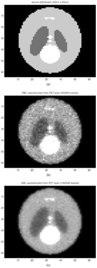
(a) A 64 × 64 source distribution in a 40 cm × 40 cm field (pixel size 6.2 mm). (b) Reconstruction using 200 000 simulated events. (c) Reconstruction using one million events. The FWHM spatial measurement resolution in the detector is 4 mm and the time resolution 0.4 ns.

C. Improved SNR Using Time-of-Flight

The crucial question for any reconstruction algorithm is the achievable image quality. As explained in Section IV, it is possible to calculate an upper bound for the estimated SNR from the information of a single dataset. A complication in this technique is the need for computing the inverse of the FIM.

This is an operation of the order O(M³), which effectively limits the evaluation of the SNR to a field of about 1000 pixels. We are, therefore, either limited to a physically small region in the source distribution or a larger field with a coarse resolution. We calculated the SNR for a 32 × 32 field of varying pixel size and, therefore, varying object size. The main interest is to demonstrate the improved image quality due to the additional time measurement.

Fig. 4 shows the resulting normalized SNR for a variety of time measurement resolutions. The SNR values are normalized by the square root of the average number of events per pixel ( $\sqrt{N/M}$). The SNR in a strict Poisson distribution is proportional to $\sqrt{N/M}$. A normalized SNR of one corresponds, therefore, to the theoretical upper limit given by Poisson statistics.

Fig. 4.

(top) SNR of the estimation of a pixel value calculated according to (23). From bottom to top the curves correspond to a pixel size of 5, 7.5, 10, and 15 mm. (bottom) SNR of the lesion detection task according to (24). The object is 16 cm × 16 cm. From bottom to top the curves correspond to a lesion diameter of 5, 10, 20, 30, 40, and 50 mm. In both cases a 32 × 32 pixel uniform distribution is used. The spatial measurement resolution has a realistic value of 0.5 cm.

For high precision in the time and space measurement the SNR reaches the theoretical limit. This corresponds to the complete knowledge of the location of the positron emission. Less precise time measurements correspond to less knowledge about where the emission occurred along the line projection given by x₁ and x₂. Note that 1 ns corresponds to 15 cm, which is roughly the object size at a pixel size of 0.5 cm. So, in this example only time resolutions better than 1 ns will improve the SNR notably at a pixel size of 0.5 cm. If the pixel size in the reconstruction is smaller than the actual spatial measurement resolution, even an exact time measurement cannot resolve the ambiguity as to where the emission originated.

Computing the inverse of the FIM limits us to a subsection of the image. For a real detector, however, one wishes to have an SNR estimate for the complete image field at the required resolution. One will choose then the SNR of the lesion detection task according to (24). Although we are not limited in the number of coordinates, we keep the 32 × 32 field for the purpose of comparison. We use now a fixed object size of 16 cm × 16 cm. The circular lesion is located at the center of the detector (and object) and has unit contrast. Fig. 4: Right shows the SNR for varying lesion diameters and varying time resolutions. The time resolutions reported in the literature range from 0.1 ns up to a few ns [17], [18]. The SNR values have been normalized by $\sqrt{N_{\text{lesion}}}$, where N_lesion, denotes the mean number of events contributing to the lesion. Again, we observe that an improved time measurement can increase the quality of the image. The two SNR measures give comparable results.

VI. Conclusion

The probabilistic description of the generation of events from a source distribution allows us to formulate an ML approach to reconstruction. Rather than binning the measurement space, the measurement coordinates can be used directly for computing the transition probabilities. No information is, therefore, lost in the binning process. This also seems advantageous in cases where the number of bins exceeds the number of detected events, which may become relevant for future detector generations in emission tomography and other modalities. In this paper, the EM scheme for solving the list-mode ML problem has been presented. An efficient technique for estimating the FIM has been presented. Ensemble statistics are circumvented by using the measured events to perform a Monte Carlo integration. Two SNR measures based on the FIM of the unbiased estimator were discussed. The SNR of a lesion detection is preferable for practical image sizes and resolutions. For both algorithms it is crucial to accurately describe the forward model of the detector in an analytic pdf. The feasibility of the proposed techniques has been demonstrated for an idealized 2-D PET detector. In particular, we show how additional measurement coordinates can improve the different SNR quality measures.

Additional research may demonstrate the technique on real detector data, while comparing its performance to binned ML reconstruction. This may further substantiate the notion that a better probabilistic model can help increase image quality.

The present limitation on biased estimators may be circumvented by using prior knowledge on the expected source distributions. In maximum a posteriori estimation (MAP) the likelihood is combined with prior distributions on the parameter f. MAP problems in the binned case have also been solved with EM algorithms [19], and possibly a similar approach could be taken here.

Fig. 2.

Sketch of the source distribution plotted together with 300 simulated events.

References

- 1.Barrett HH, Parra L, White T. List-mode likelihood. J Optical Soc Amer A. 1997;14(11) doi: 10.1364/josaa.14.002914. [DOI] [PMC free article] [PubMed] [Google Scholar]
- 2.Parra L, Barrett HH. Maximum-likelihood image reconstruction from list-mode data. J Nucl Med. 1996 June;37(5):486. in Abstracts of the 43rd Annu. Meeting of the Society for Nuclear Medicine. [Google Scholar]
- 3.Rockmore A, Macovski A. A maximum reconstruction for emission tomography. IEEE Trans Med Imag. 1982;1:113–122. doi: 10.1109/TMI.1982.4307558. [DOI] [PubMed] [Google Scholar]
- 4.Shepp L, Vardi Y. Maximum likelihood reconstruction for emission tomography. IEEE Trans Med Imag. 1982;MI-1:113–122. doi: 10.1109/TMI.1982.4307558. [DOI] [PubMed] [Google Scholar]
- 5.Lange K, Carson R. EM reconstruction algorithms for emission and transmission tomography. J Comput Assist Tomogr. 1984;8(2):306–316. [PubMed] [Google Scholar]
- 6.Lange K, Bahn M, Little R. A theoretical study of some maximum likelihood algorithms for emission and transmission tomography. IEEE Trans Med Imag. 1987;MI-6:106–114. doi: 10.1109/TMI.1987.4307810. [DOI] [PubMed] [Google Scholar]
- 7.Chornoboy E, Chen C, Miller M. An evaluation of maximum likelihood reconstruction for SPECT. IEEE Trans Med Imag. 1990;9:99–110. doi: 10.1109/42.52987. [DOI] [PubMed] [Google Scholar]
- 8.Snyder D, Politte D. Image reconstruction from list-mode data in an emission tomography system having time-of-flight measurements. IEEE Trans Nucl Sci. 1983 June;NS-20:1843–1849. [Google Scholar]
- 9.Cover T, Joy A. Elements of Information Theory. New York: Wiley; 1991. [Google Scholar]
- 10.Barrett H, Denny J, Wagner R, Myers K. Objective assessment of image quality II: Fisher information, Fourier crosstalk and figures of merit for task performance. J Optical Soc Amer A. 1995;12(5):834–852. doi: 10.1364/josaa.12.000834. [DOI] [PubMed] [Google Scholar]
- 11.Dempster A, Laird N, Rubin D. Maximum likelihood from incomplete data via the EM algorithm. J Roy Stat Soc B. 1977;39:1–38. [Google Scholar]
- 12.Lange K, Carson R. EM reconstruction algorithm for emission and transmission and tomography. J Comput Assist Tomogr. 1984;8(2):306–316. [PubMed] [Google Scholar]
- 13.Berger J. Statistical Decision Theory and Bayesian Analysis. New York: Springer-Verlag; 1985. [Google Scholar]
- 14.Chen C, Metz C. A simplified EM reconstruction algorithms for TOFPET. IEEE Trans Nucl Sci. 1985 Feb;NS-32:885–888. [Google Scholar]
- 15.Politte D, Hoffman G, Beecher D, Ficke D, Holmes T, Ter-Pogossian M. Image-reconstruction of data from SUPERPETT I: A first-generation time-of-flight positron-emission-tomograph. IEEE Trans Nucl Sci. 1986 Feb;NS-33:428–434. [Google Scholar]
- 16.Ishii K, Orihara H, Matsuzawa T. Construction function for three-dimensional sinograms of the time-of-flight positron transmission tomography. Rev Scientific Instrum. 1987;58(9):1699–1701. [Google Scholar]
- 17.Robeson W, Dhawan V, Takikawa S, Babchyck B, Anazi I, Margouleff D, Eidelberg D. SUPERPETT 3000 time-of-flight PET tomograph: Optimization offactors affecting quantization. IEEE Trans Nucl Sci. 1993 Apr;40:135–142. [Google Scholar]
- 18.Tzanakos G, Bhatia M, Pavlopoulos S. A Monte Carlo study of the timing resolution of BaF;i2 for TOF PET. IEEE Trans Nucl Sci. 1990 Oct;37:1599–1604. [Google Scholar]
- 19.De Pierro A. A modified expectation maximization algorithm for penalized likelihood estimation in emission tomography. IEEE Trans Med Imag. 1995 Feb;14:132–137. doi: 10.1109/42.370409. [DOI] [PubMed] [Google Scholar]