Automated Measurement and Statistical Modeling of Elastic Laminae in Arteries

Abstract

Structural features of elastic laminae within arteries can provide vital information for both the mechanobiology and the biomechanics of the wall. In this paper, we propose, test, and illustrate a new computer-based scheme for automated analysis of regional distributions of elastic laminae thickness, inter-lamellar distances, and fragmentation (furcation points) from standard histological images. Our scheme eliminates potential artifacts produced by tissue cutting, automatically aligns tissue according to physiologic orientations, and performs cross-sectional measurements along radial directions. A statistical randomized complete block design (RCBD) and F-test were used to assess potential (non)-uniformity of lamellar thicknesses and separations along both radial and circumferential directions. Illustrative results for both normotensive and hypertensive thoracic porcine aorta revealed marked heterogeneity along the radial direction in nearly stress-free samples. Clearly, regional measurements can provide more detailed information about morphologic changes that cannot be gained by globally averaged evaluations alone. We also found that quantifying Furcation Point densities offers new information about potential elastin fragmentation, particularly in response to increased loading due to hypertension.

1. Introduction

Of the many structural constituents that make up the arterial wall, elastin plays a particularly important role in large arteries. Elastin endows these arteries with considerable distensibility, elasticity, axial prestretch, and overall durability; it similarly provides important biological cues for associated smooth muscle cells to remain quiescent and contractile [1, 2]. Not surprisingly, therefore, mounting laboratory and clinical evidence shows that damage to or loss of elastin contributes significantly to many arterial pathologies. For example, fatigue-induced fragmentation and degeneration of elastin are major contributors to the increased caliber, neointimal thickening, tortuosity, and stiffening that are hallmarks of arterial aging [3, 4], and thereby contribute to the associated increased pulse pressure and risk of heart attack, stroke, and kidney failure [5, 6]. Indeed, similar changes in elastin cause or are caused by hypertension and thereby contribute to its devastating role in the progression of many cardiovascular diseases [7]. Increasing evidence also suggests that a deficiency of fibrillin-1 (an elastin associated glycoprotein) in people having Marfan syndrome renders the arterial elastin more susceptible to degeneration and enzymatic degradation [8], which in turn contributes to dilatation and eventual dissection of the ascending aorta. Degradation and loss of elastin is similarly thought to play a key role in the pathogenesis and subsequent enlargement of both abdominal aortic and intracranial aneurysms [9, 10], and it appears to play a role in both the development of atherosclerosis [11] and the restenosis that often follows balloon angioplasty or intravascular stenting [12]. There is, therefore, a pressing need to quantify changes in elastin organization within the arterial wall.

Histological and immunohistochemical methods continue to provide valuable information on the architecture of the arterial wall, including elastin. In particular, histological features such as the thickness of the elastic laminae, inter-lamellar separations, fragmentation, and localized loss of elastin are important diagnostic metrics. There is a pressing need, however, to extract such information from histological images in a more objective as well as time- and labor-efficient manner. Robust computer-aided measurement and modeling of elastic laminae thus has an important role to play in both vascular pathology and vascular mechanics. In this paper, we propose an image analysis scheme to delineate spatial distributions and altered patterns of elastic laminae, including changes in thickness, spacing, and fragmentation. In particular, key contributions of our automated scheme include: (1) A Radon Transform (RT) based technique to identify principal (i.e., major) directions of the laminae, (2) regional measurement techniques for lamina thickness (LT) and inter-lamellar distances (ILD), (3) furcation point (FP) detection and spatial measurements of density distributions, and (4) statistical based experimental design to validate hypotheses related to regional non-uniformity of the elastic laminae in aorta. The approach presented in this paper thus enables a fully automated analysis system that includes elastic laminae extraction, alignment, point-wise and transmural thickness measurement, and statistical hypothesis testing to assess the (non)-uniformity of LT and ILD. The basic measurement technique was presented at an IEEE Symposium [13], but the uniformity analysis of LT is the first of its kind; it complements the homogeneity analysis of elastic laminae based on mechanical experiments [14]. It is also shown here that although automatic alignment of arterial sections by principal direction of elastic laminae is complicated by their inherent waviness, sectioning artifacts, and arbitrarily oriented specimens, a RT based algorithm can align histological images (typically 1500×2000 or larger) faster than traditional approaches such as linear fitting [15], eigenvector/eigenvalue analysis [16], and texture orientation measurement methods [17-21]. Moreover, the RT method also works well when the noise level is low and the image size is small, hence rendering it useful in general.

2. Methods

2.1 Image preparation and system flowchart

Cylindrical segments of excised porcine thoracic aorta from another study [22] were cut to release residual stresses and processed using standard histological methods (e.g., embedded, sectioned, and stained). Sections were stained with Verhoeff Van Gieson (VVG) to focus on intramural elastin (the main component of elastic laminae). Images were acquired using a research light microscope (Olympus BX51) coupled with a digital camera (Olympus DP70). The 1360 × 1024 digitized images were taken at 1/500 second exposure time, ISO 200 sensitivity, and 20x zoom. When necessary, the “PanaVue Image Assembler” was used to stitch together snapshots to form a whole section of the aortic wall. All images were rotated into the same sequence of the three main layers (left to right): adventitia (outer layer), media (middle layer), and intima (inner layer), with attention directed primarily to the elastin-rich media (Figure 1). Note, therefore, that the elastic laminae are represented by the dark lines in Figure 1 whereas the pink/purple denotes remaining constituents, primarily collagen, smooth muscle, and ground substance matrix. The overall processing flow of the automated analysis system is depicted in Figure 2.

Figure 1.

Light microscopic images of representative cross-sections of porcine thoracic aorta in a nearly stress-free configuration in (a) normotension (NT) and (b) 4-week hypertension (HT). Note the typical tri-layered structure (adventitia, media, and intima). The intramural constituents include the concentric elastic laminae (dark lines) and intra-lamellar smooth muscle, collagen, and ground substance (pink). Two delimiting elastic laminae and the enclosed tissue define the basic structural and functional unit of the wall, a musculo-elastic fascicle or lamellar unit. The principal (circumferential) direction runs along the trajectory of elastic laminae whereas the perpendicular (radial) direction runs radially from intima to adventitia.

Figure 2.

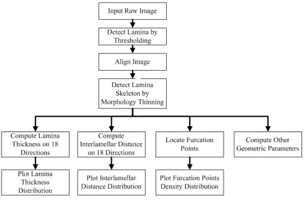
Processing flow for automated elastic laminae structural analysis.

2.2 Lamina detection

It is relatively simple to extract elastic laminae from an original image when there is a sharp contrast between each lamina (foreground) and the non-elastin lamellar (background) constituents, particularly in the red channel of color images (Figure 3a). Yet, different threshold selections can yield different segmentation outcomes. For example, referring to a histogram for a representative histological sample (Figure 3b), there is a clear, but not distinct, boundary between foreground and background. To avoid the need for manual selection and decisions on the appropriate dividing threshold, we adopted an adaptive threshold method [23] to segment the foreground (elastic laminae) and background:

1. Empirically set an initial threshold I₀ to 140.

2. Segment image pixels as foreground or background based on I₀.

3. Compute the average intensity of pixels in the foreground as I₁ and that of background as I₂.

4. Compute a new threshold $I_0^{\prime }=\frac{(I_1+I_2)}{2}$

5. If$\mid I_0-I_0^{\prime }\mid <1$, then stop. Else, let $I_0=I_0^{\prime }$ and go back to step 2.

Next, $I_0^{\prime }$ was used as a threshold to eliminate the background and generate a binarized map of the elastic laminae (Figure 3c). Small laminae (≤ 20 pixels) were assumed to be cutting artifacts or marginal tissues, and were either removed (laminae) or filled (inter-lamellar regions) with a seed fill [23]. Centerlines (skeleton) of the elastic laminae (Figure 3d) were then extracted using a mathematic morphology based thinning algorithm [24, 25]. Once this step was completed, it was then possible to determine the mean principal direction (i.e., direction of primary “flow”, typically circumferential in an artery) of the elastic laminae (Figure 1) and then to determine other metrics of interest along the perpendicular direction (typically radial in an artery). The associated techniques to compute these metrics are discussed in order below.

Figure 3.

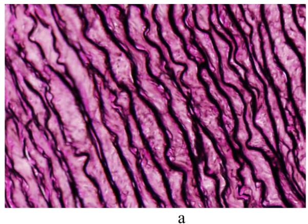
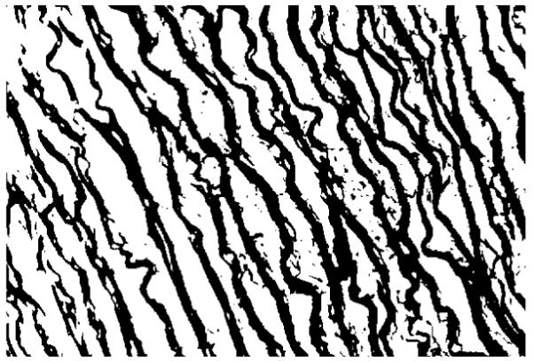
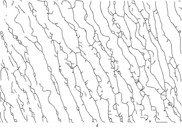
(a) A representative non-aligned portion of an aortic cross-section, (b) an intensity histogram for the red channel from the raw image (x-axis is the grayscale intensity range [0 255], y-axis is the counts of image intensity), (c) the binarized map highlighting the elastic laminae, with an adaptive threshold = 121 (black area), and (d) a skeleton map of the laminae with artifacts (black lines).

2.3 Principal direction of elastic laminae

In [13], we proposed an algorithm using an energy function derived from the well known RT (Radon Transform) to find the principal laminae direction, which is defined as the majority flow direction. The energy function was defined as:

$$e\left(\theta \right)\left\{RT\left[f(x,y)\right]\right\}={\parallel \nabla \left\{R{T}_{\theta }\left[f(x,y)\right]\right\}\parallel }^2,$$ (1)

where ∇(·) = d (·)/dθ, f is a function, (x,y) is the coordinate of a laminae point, and θ is the radon transform projection angle. By modeling elastic laminae as rectangular objects, the RT-based energy function becomes

$$E_{RT}(x,y)={\int }_{-\infty }^{\infty }{\left[\frac{d{g}_{\pi }(x,y)}{dr}\right]}^{2}dr,$$ (2)

where r is the perpendicular distance from the origin to the straight line, with integration limits to infinity based on definition of radon transform, and

$$g_{\pi }(x,y)=\tan \theta \{\mathrm{sgn}\left[(p\csc \theta +b)ctg\theta a\right]\min [\mid p\csc \theta +b\mid ,\mid ctg\theta a\mid ]-\mathrm{sgn}\left[(pcsc\theta -b)ctg\theta a\right]\min (\mid p\csc \theta -b\mid ,\mid ctg\theta a\mid )\},$$

where tan(·) is the tangent function, sgn(·) is the sign function, csc(·) is the cosecant, ctg(·) is the cotangent function, a is a constant which is obtained from the rectangle function, with distance p and angle θ defining the straight line.

To verify the accuracy of our automatic method, we randomly picked 40 sample images and a “blinded” expert manually selected a principal direction three times. Difference between the average results for the manual and automatic methods are summarized in Table 1. The mean and standard deviation of the differences is 1.6±1.0 degrees.

Table 1.

Comparison of principal directions determined by manual and automatic measurement

Sample #	1	2	3	4	5	6	7	8	9	10
Measure 1	−25	−16	−16	24	28	13	15	−12	23	25
Measure 2	−24	−14	−14	25	29	12	16	−10	28	28
Measure 3	−25	−13	−13	25	28	13	15	−10	21	22
Auto Measurement	−24	−12	−12	26	27	14	15	−10	26	22
Difference	0.7	2.3	2.3	1.0	1.0	1.3	0.3	1.0	2.0	3.0
Sample #	11	12	13	14	15	16	17	18	19	20
Measure 1	21	−22	−20	−19	−9	8	11	10	14	18
Measure 2	22	−21	−21	−18	−10	9	12	12	15	19
Measure 3	21	−23	−23	−20	−10	10	11	11	15	20
Auto Measurement	25	−19	−19	−18	−9	10	9	9	15	18
Difference	3.7	3.0	2.3	1.0	0.7	1.0	2.3	2.0	0.3	1.0
Sample #	21	22	23	24	25	26	27	28	29	30
Measure 1	15	17	10	5	21	−31	−28	−41	−20	11
Measure 2	14	16	11	4	25	−30	−25	−40	−21	11
Measure 3	14	17	11	3	23	−30	−24	−40	−19	10
Auto Measurement	13	18	11	1	20	−29	−23	−43	−22	10
Difference	1.3	1.3	0.3	3.0	3.0	1.3	2.7	2.7	2.0	0.7
Sample #	31	32	33	34	35	36	37	38	39	40
Measure 1	−20	15	−25	−23	−26	23	−22	−14	−10	−15
Measure 2	−24	17	−26	−21	−27	24	−20	−15	−9	−11
Measure 3	−23	17	−27	−22	−27	25	−23	−15	−10	−13
Auto Measurement	−20	16	−26	−22	−23	23	−19	−12	−9	−12
Difference	2.3	0.3	0.0	0.0	3.7	1.0	2.7	3.0	1.0	1.0

Furthermore, we tested the RT algorithm and evaluated its accuracy by comparing results to those for a LF (linear fitting) algorithm using a known, synthetic binary image (Figure 4). Each curve within the synthetic image was created using five different functions so that their shapes resemble that of elastic laminae. The functions are (from top to bottom):

$$\begin{array}{c}{y}_1=0.6\sin \left(0.5x\right)+0.25\sin (0.3x-3)+\sin (0.1x-4)\hfill \\ y_2=0.6\sin (0.5x-3)+0.25\sin (0.3x+3)+\sin (0.1x-4)\hfill \\ y_3=0.3\sin (0.6x-3)+0.5\sin (0.71x-3)+0.9\sin (0.21x+4)\hfill \\ y_4=0.36\sin (0.7x-1)+0.75\sin (0.41x-2)+0.27\sin (0.25x+1)\hfill \\ y_5=0.41\sin (0.19x-1)+0.5\sin (0.51x+2)+0.3\sin (0.65x-1).\hfill \end{array}$$ (3)

Figure 4.

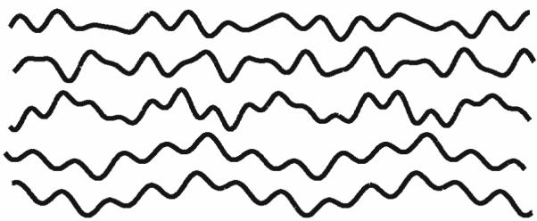
A synthetic binary image consisting of five sinusoidal curves that was used to verify the accuracy of our Radon Transform (RT) algorithm. The principal directions of all curves were forced to be 0° from horizontal, but the image was rotated by 30°, 60°, 90°, 120°, 150° or 180° for different tests. After repeating ten times for each rotation, averaged outcomes for both RT and linear fitting (LF) algorithms were compared to assess their accuracies.

All of the synthetic curves were created so that their principal directions had an initial zero degree orientation relative to horizontal. We then generated test images by rotating the original images from 30° to 180°, in 30° increments. Averages of ten experimental runs for RT and LF fitting methods are in Table 2, which reveals that the RT algorithm was consistently more accurate than the LF algorithm as expected.

Table 2.

Comparison between the given principal direction and outcomes from RT and LF algorithms

True Rotation Degree θ0(°)	LF result θ1 (°)	LF Accuracy (%)	RT result θ2 (°)	RT Accuracy (%)
30	30.11	0.4	30	0.0
60	59.9	−0.2	60	0.0
90	94.2	4.7	92	2.2
120	120.51	0.4	120	0.0
150	150.31	0.2	150	0.0
180	180.17	0.1	180	0.0

Column one is the rotated degrees of Figure 4 from the prescribed principal direction. Columns two and four are, respectively, the principal directions computed by the LF and RT algorithms. The accuracies (θ₁−θ₀)/θ₀ are listed in columns three and five as percents.

Furthermore, we chose five “representative” aortic cross-sectional images having the same resolution but different dimensions to compare the performance of these two methods. The LF scheme generated principal directions with good accuracy when the threshold for the laminae skeleton length (cf. Figure 3d) was selected properly. Figure 5 illustrates the relationship between skeleton length threshold and estimated principal direction (for Figure 3a) using the LF method, with the threshold chosen to be 10 to 65 pixels with a 5-pixel increment. Maximum and minimum vales were 27.02° and 35.89°, that is, about 8° different. Indeed, the estimated principal direction tended to a converged value even for large thresholds (> 40). Proper parameter selection for the LF-based algorithm is not an easy task, however. In contrast, the RT-based algorithm does not require thresholding; the input can be a grayscale image and the RT-based algorithm is shift-, rotation- and scale-free. We always obtained little error in the numerical experiments when removing any combination of the five curves.

Figure 5.

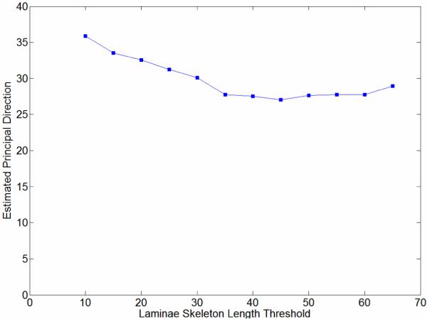
Computed angle for the principal (circumferential) direction estimated by the LF-based method for the aortic image in Figure 3a, using different laminae skeleton length thresholds. The largest and smallest angles were 35.89° (threshold 10 pixels) and 27.02° (threshold 45), respectively. The associated parameter-insensitive angle computed using the RT method was 27°.

Finally, when smaller laminae were removed based on a length threshold of 20 pixels, the remaining laminae skeleton was fit to a linear equation having slope k and y-intercept b (i.e., y = kx + b). The direction of every fit line is tan⁻¹(k). With all laminae fit, we chose the median value of all directions as the principal direction of the elastic laminae within the cross-sectional image. Accuracies and computing times for the RT-based algorithm were compared against the LF-based method (Table 3), with computation time averaged over the five different runs for each image. As it can be seen from the table, the RT-based method also had a marked speed gain over the LF counterpart. Given that most aortic images are large (e.g., 1360 × 1024), the RT-based method was found to be more suitable for large scale experiments.

Table 3.

Computation time and accuracy comparison between LF and RT-based algorithms

	Computing Time			Measurement Results
Sample (dimension)	LF Method Time t1(sec)	RT Method Time t2(sec)	Time Ratio (t2/ t1)	PD from Linear Fitting P1 (°)	PD from RT P2 (°)	PD error (P1-P2)
1 (563 × 500)	4.565	5.97	1.31	78.5	80	−1.5
2 (637×474)	5.025	6.71	1.33	88.2	87	1.2
3 (806×744)	14.33	14.25	0.99	81.8	81	0.8
4 (1866×1372)	118.78	66.32	0.56	77.5	77	0.5
5 (2513×1382)	199.47	107.2	0.54	83.8	83	0.8

Column one is the number of sample images and their sizes (measured by pixel count). Columns two and three are the computing times for the two algorithms: linear fitting (LF) and Radon transform (RT). Columns five and six are the angles of the principal directions (PD) computed by the two algorithms. The last column is the difference between the results of the two methods. Despite similar accuracies, the RT based method outperformed the LF method because of its lower processing time for large images.

2.4 Lamina thickness sampling method, estimation, and experimental model

We adopted the definitions of LT (laminae thickness) and ILD (inter-lamellar distances) from [26], where LT is the shortest distance between two elastic laminae boundaries and ILD is the shortest distance between two neighboring laminae, and we used the method in [27] to measure the LT and ILD. Point-wise measurements of LT were based on a local search method along 18 directions within the cross-sectional image plane [13]. The ILD can be measured similarly for regions between neighboring elastic laminae. To verify the accuracy of this method, we randomly picked 97 points from seven different sample images. We compared the manual IL measurement with the automatic method; the difference was 0.4±0.3 pixels, which showed the reliability of our algorithm.

A more challenging issue, however, was to assess the (non)-uniformity of LT distributions across different regions. If LT was mostly homogenous, a simple average of all point-wise measurements would suffice. Otherwise, regional measurements of LT would be required to study structural characteristics of LT across the wall. Because one can derive an overall average from regional measurements, we based our study on regional analysis techniques. Specifically, to determine possible regional homogeneities, one could first divide each image using r uniform vertical blocks that have the same heights as the image height, and then analyze the LT statistics in each block. Because such blocks could have different numbers of observations, however, this naïve approach could lead to biased statistical estimations. To eliminate such potential biases, we employed a randomized complete block design (RCBD) [28, 29] with a fixed number t of samples in each block to test the homogeneity hypothesis. RCBD is one of the simplest blocking designs to control and reduce experimental errors. Our analysis is confined to a 1D (vertical or horizontal) homogeneity analysis and consists of two steps (Figure 6): RCBD and standard F-test checks of homogeneity.

Figure 6.

Homogeneity test using both a Randomized Complete Box Design (RCBD) and a statistical F-test.

Based on the central limit theorem, one can assume that the measurement L over a homogenous area to be an independent and identically distributed random variable with a small standard deviation. For a randomly selected number t (not independent and identically distributed in different areas) of samples L₁, L₂, …, L_t within an analysis region w, the measurement mean $\stackrel{‒}{L}=\frac{1}{t}{\sum }_{i=1}^t{L}_i$ approaches that for a Normal distribution N(μ,σ(t)), where μ and σ(t) are the usual mean and standard deviation. Equal size t can help yield reasonably small variance in all analysis areas. The aforementioned RCBD method was thus applied to reduce variations for experimental results on the distributions of transmural metrics of interest. The parameters for the RCBD are summarized in Table 4.

Table 4.

Statistical Randomized Complete Block Design (RCBD) for hypothesis testing of equal measurement means

measurement	region 1	region 2	…	region r	measurement means
1	y11	y12	…	y1r	${\stackrel{‒}{y}}_{1•}$
2	y21	y22	…	y2r	${\stackrel{‒}{y}}_{2•}$
…	…	…	…	…	…
t	yt1	yt2	…	ytr	${\stackrel{‒}{y}}_{t•}$
block means	${\stackrel{‒}{y}}_{•1}$	${\stackrel{‒}{y}}_{•2}$	…	${\stackrel{‒}{y}}_{•r}$	${\stackrel{‒}{y}}_{••}$

The sample images are divided into r vertical regions (blocks) with heights equals to the image height. In each region, we randomly pick t measurements, e.g. LT or ILD. y_ij is the j^th measurement in the region i. ${\stackrel{‒}{y}}_{i•}$ is mean of ith measurement within all regions, ${\stackrel{‒}{y}}_{•j}$ is mean within region j, and ${\stackrel{‒}{y}}_{••}$ is estimated true means of all measurements.

In particular, we partitioned the medial layer into r non-overlapped columns (blocks) with the number of entries equaling the image height. In each region, we randomly picked t measurements (rows) where t =10n̄ and n̄ is the average number of sampling points over r regions within the whole image. Because the physical width of the regions could become unequal, the same number t of samples was used in each observation. We then applied a linear model for the i^th parameter measurement (i.e., diagnostic metric) within the j^th analysis region (block):

$${\nu }_{ij}=\mu +{\tau }_i+{\rho }_i+e_{ij},$$ (4)

where i = 1,2,…,t, j=1,2,…,r, μ is the true measurement mean, ρ_i is the treatment effect which explains how much a measurement changes on an experimental unit and e_ij is the measurement error. The block effect ρ_j is the average deviation of L from μ within each analysis region (block) j. Recall that the number of analysis regions is r and the number of sampling points in each region is t. For simplicity, we assumed random sampling point locations. The measurement error e_ij was thus assumed to be distributed normally with zero mean and a common variance. The F statistic [28] used to test hypothesis H₀ was:

$$F_0=\frac{MST}{MSE}=\frac{r\sum _{i=1}^t{({\stackrel{‒}{y}}_{i•}-{\stackrel{‒}{y}}_{••})}^2∕(t-1)}{\sum _{i=1}^t\sum _{j=1}^r{(y_{ij}-{\stackrel{‒}{y}}_{i•}-{\stackrel{‒}{y}}_{•j}+{\stackrel{‒}{y}}_{••})}^2∕\left[(r-1)(t-1)\right]},$$ (5)

where ${\stackrel{‒}{y}}_{i•}$ is i^th measurement mean, ${\stackrel{‒}{y}}_{••}$ is the estimated general mean, ${\stackrel{‒}{y}}_{•j}$ is the j^th block mean, and y_ij is the measurement at i^th location and j^th block.

We used ANOVA [28] (analysis of variance) statistics to analyze results for LT and ILD in regions derived from the RCBD. The F statistic was used to test the null hypothesis H₀: H₀: μ₁= μ₂=…= μ_i, where μ_i is the mean of LD or ILD at block i. We wanted to test whether or not there were significant differences between the measurement means along the principal (or, circumferential) and radial directions at a significant level α = 0.05. The test statistic α is the probability of exceeding the value of the test under the null hypothesis. The value labeled Prob > F in the last column of Table 5 is often referred as the “P-value”. In this paper, we chose the traditional significance level 0.05.

Table 5.

ANOVA tables for normotension and 4-week hypertension LT and ILD data

(a) ANOVA of the normotension LT data.
Source	Sum Square Error	Degree of Freedom	Mean Square Error	F-Statistics	Prob > F
Blocks	27121.5	193	140.526	36.93	0
Rows	1849.2	546	3.387	0.89	0.9687
Errors	400946.3	105378	3.805
Total	429917	106117
(b) ANOVA of the 4-week hypertension LT data.
Source	Sum Square Error	Degree of Freedom	Mean Square Error	F-Statistics	Prob > F
Blocks	39078.3	207	188.784	42.34	0
Rows	1616.1	344	4.698	1.05	0.2377
Errors	317531.4	71208	4.459
Total	358225.8	71759
(c) ANOVA of the normotension ILD data.
Source	Sum Square Error	Degree of Freedom	Mean Square Error	F-Statistics	Prob > F
Blocks	1453516	193	7531.17	96.67	0
Rows	44104.2	637	69.24	0.89	0.9794
Errors	9578285.7	122941	77.91
Total	11075905.9	123771
(d) ANOVA of the 4-week hypertension ILD data.
Source	Sum Square Error	Degree of Freedom	Mean Square Error	F-Statistics	Prob > F
Blocks	1189810.3	206	5775.92	87.87	0
Rows	20542.8	375	54.78	0.83	0.9916
Errors	5077828.7	77250	65.73
Total	6288211.7	77831

ANOVA (analysis of variance) in tables (a-d) test the homogeneity of LT or ILD under normotension (NT) and hypertension (HT) along different directions. Column six explains the probability of homogeneity. If the probability is larger than α, we cannot reject the null hypothesis (no significant differences between the measurement means along the principal (circumferential) or radial direction) at α level. Otherwise, we might conclude heterogeneity. In rows two and three of each table, the block and row effects test the homogeneity along the radial and principal directions, respectively. Based on above definitions, LT and ILD are homogeneous along the circumferential direction for both the NT and HT cases. In contrast, LT and ILD are heterogeneous along the radial direction for both NT and HT.

A detailed analysis of LT and ILD was completed for one representative normotensive (NT) and one 4-week hypertensive (HT) sample (Table 5). For both NT and HT, we found LT to be significantly different among blocks (F = 0 < α) at α = 0.05, which implied that LT was not distributed uniformly along the radial direction. In contrast, the F-statistics for LT and ILD were all larger than α = 0.05 which suggested that LT or ILD were distributed uniformly along the circumferential direction for both the NT and 4-week HT cases. Their F-statistics are 0.9687, 0.2377, 0.9794 and 0.9916 respectively.

Furthermore, comparison of images from 5 NT and 21 HT thoracic aortas revealed the following two key results:

Result 1: LT and ILD exhibited regional heterogeneity along the radial direction for both NT and HT cases. All samples provided consistent F-statistics (close to 0) to support the heterogeneity hypothesis of LT and ILD distributions.

Result 2: LT and ILD exhibited regional homogeneity along the circumferential direction for both NT and HT cases. F-statistics of most samples were larger than α = 0.05 (4/5 NT for LT and 3/5 NT for ILD, and 16/21 HT for LT and 18/21 HT for ILD). These results suggested that, in most cases, LT and ILD can be considered uniformly distributed along the circumferential direction under both NT and HT.

It is cautioned, however, that these results hold for the specific samples considered and should not be thought to be true for all loading conditions for all aortas or aortic segments in general. Nevertheless, despite our fundamentally different methods of analysis, our findings are consistent with those of [14, 22, 30], that is, LT is not uniformly distributed along the radial direction in general. As such, gross averages of point-wise measurements may fail to detect subtle changes of LT and ILD with time or location within the wall. The evaluation outcomes also validate the usefulness of the computer-based analysis scheme, hence it can be applied reliably to large scale studies.

Figure 7 illustrates representative distributions of LT and ILD along the radial direction of a NT (Figure 7a) and a 4-week HT (Figure 7b) aorta sample, where the x-axis denotes a normalized media layer coordinate and the y-axis the averaged LT (with the unit of measurement per pixel). All observations were normalized onto a [0,1] range to facilitate comparison between samples. Figure 7 (c) and (d) show the corresponding distributions of ILD from the same samples. Clearly, neither the LT nor the ILD distributions through the wall were uniform, consistent with the outcome of the hypothesis testing. The average LT was only slightly higher for the HT (= 4.32) than the NT (=3.81) aortas, but there was a tendency toward a higher value toward the lumen in the hypertensive cases (Figure 7b).

Figure 7.

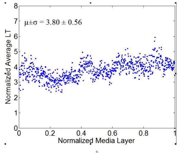
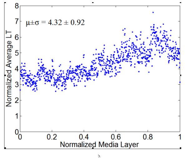
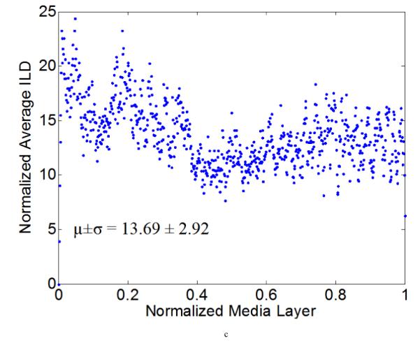
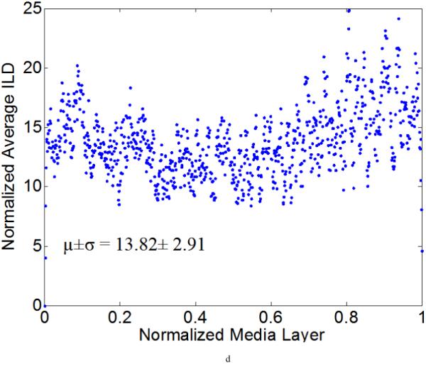
Computed elastic laminae thicknesses (a, b) and inter-lamellar distances (c, d) within the medial layers of representative normotensive (a,c) and 4-week hypertensive (b,d) thoracic aorta. Every point represents the average measurement within an analysis window for a fixed number of samples. Both the measurement locations (x-axis) and the measurements themselves (y-axis) were normalized to facilitate sample-to-sample comparisons; each data point is the result of the actual measurement divided by the maximum value of all measurements. The global mean and standard deviation of actual measurements are given at the bottom of each figure.

Various system indicators (or metrics) can be derived from the basic thickness maps for the elastic laminae. For instance, three different maps can be generated easily to visualize thickness patterns at a coarse level (Figure 8), where elastic laminae thickness LT is quantized into “below average” (LT < μ-σ), “average” (μ-σ < LT < μ+σ), and “above average” (LT > μ+σ). Visual inspection suggested that elastic laminae in the “below average” and “average” maps were fairly uniform whereas those in the above “average” map were less so. In other words, the non-uniform distribution of LT appeared to be due to those laminae having a greater thickness, particularly in hypertension.

Figure 8.

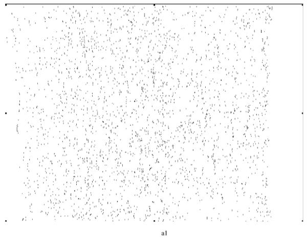
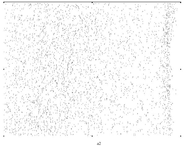
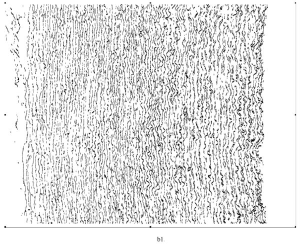
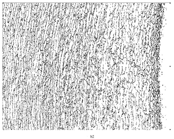
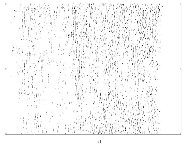
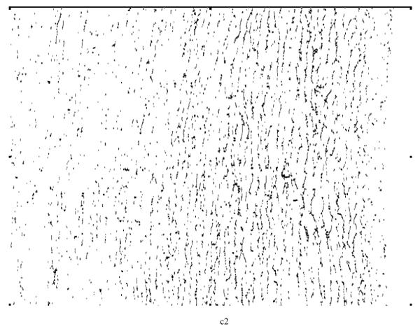
Regional, spatial non-uniformities of the laminae thickness (LT) illustrated by a simple thresholding routine: (a) below average (LT < μ−σ), (b) average (μ−σ < LT <μ+σ), and (c) above average (LT > μ+σ).

2.5 Aortic fragmentation measured via furcation point densities

A furcation point (FP) is a point at which an elastic lamina divides into two or more branches. The FP density could thus indicate fragmentation, or tearing, of elastic laminae under different conditions. Although general techniques for detecting vascular networks [31, 32] can be used for FP detection, they are not applicable for our needs. For example, the common practice of merging closely located bifurcation points (bi-FPs) would introduce significant errors, and modeling bi-FPs as a supremum of openings having a morphological T shape [31] would introduce significant artifacts. Rather, we followed the basic model of FP detection described in [31] and used matching of templates (see Figure 9) within 3x3 analysis windows on the elastic laminae skeletons to get our results.

Figure 9.

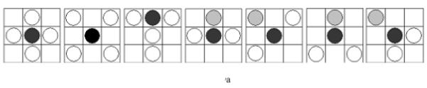
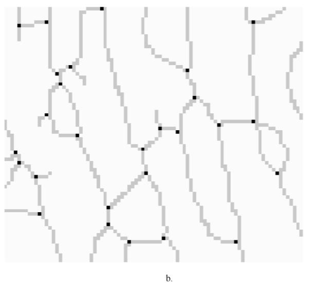
(a) Furcation Point (FP) Analysis using 22 standard templates (note: the first two patterns from the left allow one configuration each whereas the third to the seventh patterns allow four different orientation situations each). These templates were trained using sample images to locate furcation points, denoted by a black circle. A grey circle denotes a skeleton pixel not on a furcation point, and a hollow circle denotes a skeleton pixel. The block need not be considered if it does have any of the marks mentioned above. (b) Furcation points (marked in black dots) detected from skeleton lines (marked by light gray lines) for a representative magnified local section from an aortic image.

By visual inspection, we found that the 22 templates defined in Figure 9a (note: the first two patterns have only one configuration, but the third to the seventh patterns have four orientations) were adequate for our needs, where a hollow circle is a skeleton pixel only, a gray circle is a skeleton pixel that cannot be a furcation point, and a solid black circle is a furcation point. Based on initial FP detection, as illustrated in Figure 9b, we computed the FP area density ${\mu }_{S,FP}=(1∕S_{CS}){\sum }_{i=1}^n{w}_i$ and line density ${\mu }_{L,FP}=(1∕L_{EL}){\sum }_{i=1}^n{w}_i$, where n is the total number of FPs within a designated analysis area. S_CS is the total analysis surface area, L_EL is the total length of elastic laminae within S_CS, and w_i is the weight of the i^th FP (the weight of a FP with m+1 branches is m−1, for example, a bi-FP has three branches and a weight of one). These two densities could be used to characterize elastin fragmentation or perhaps incompletely deposited fibrils under different conditions. Illustrative results are shown in Table 6 and Figure 10 for five classes of aortic samples: surgical controls (normotensive) and 2-, 4-, 6- and 8-week hypertensive (HT) samples. As it can be seen, the longer durations of hypertension resulted in larger differences in both FP metrics from control values, thus suggesting either greater fragmentation or perhaps the deposition of new elastic fibers that were not incorporated completely within extant laminae. Note that these differences are reflected by the changes Δ_S and Δ_L relative to the surgical controls (SC).

Table 6.

Area and line density of furcation points corresponding to Figure 10

	μS,FP (10-3)	N	ΔS (%)	μL,FP (10-2)	N	ΔL (%)
SC	2.62±0.26	17		3.98±0.15	14
2-W	2.46±0.23	14	−5.86	4.03±0.30	17	1.44
4-W	2.53±0.28	13	−3.32	4.17±0.25	10	4.89
6-W	1.99±0.32	14	−23.87	3.62±0.34	15	−9.05
8-W	1.31±0.20	19	−49.93	3.3±0.24	16	−17.09

We list five groups of aorta in this table: surgery control (SC, which is normotensive), 2-week, 4-week, 6-week and 8-week hypertension (HT). The second and fifth columns are the FP area and line density measurements, average and standard deviation. The third and sixth columns are the sample image counts used in each group. The fourth and seventh columns are differences relative to results for SC. We found μS,FP (furcation point area density) to decrease monotonically with the duration of HT and μL,FP (furcation point line density) to increase slightly at 2- and 4-weeks, then decrease sharply.

Figure 10.

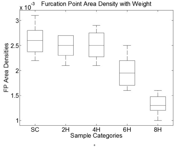
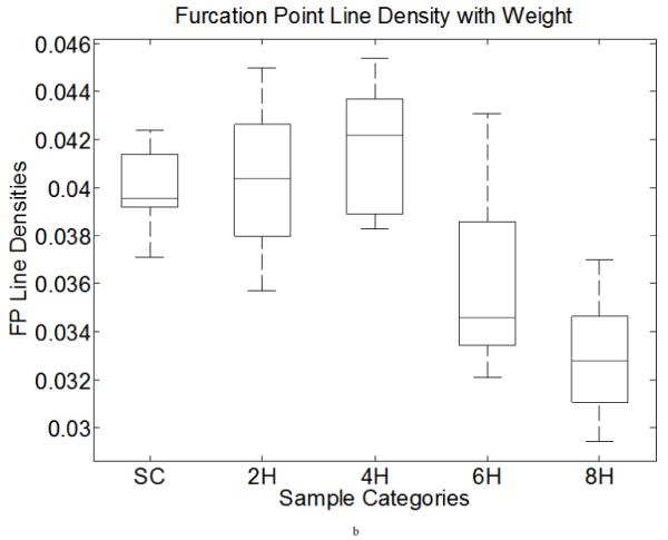
Furcation point area (line) density boxplots of data from Table 6. Both computations include five categories: surgery control (SC) and two-, four-, six- and eight-week HT aortic samples. X-axis shows the categories, y axis demonstrates the FP area (left) and line (right) densities. The middle line in each box is the median within each group. The upper and lower bound of each box is the lower (25%) and upper (75%) quartile.

The FP area density distribution was relatively uniform under normotensive conditions (Figure 11a), but there was a spiked local increase and global elevation within the central region in hypertensive specimens (Figure 11b). It is not clear why there was more pressure-induced remodeling within the middle region of the media under hypertension while regions closer to intima and adventitia were less affected, but these are the types of observations that are needed to generate new hypotheses for the mechanobiology.

Figure 11.

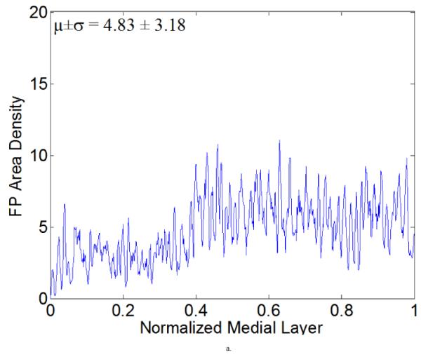
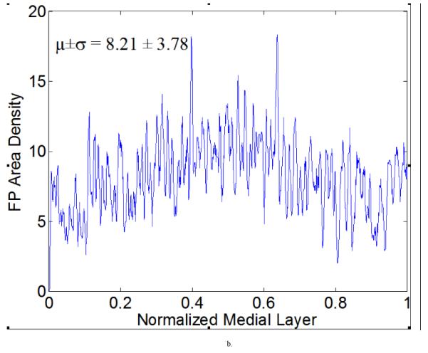
Furcation point (FP) area density measurements with a running average (window size is five) for representative (a) normotensive and (b) 4-week hypertensive samples. These results show a higher mean value of FP area density for the hypertensive sample, with a significant increase within the middle of the medial layer. Such measurements can be used to generate higher order statistics if desired.

Finally, although not shown, the mean length of elastic laminae was slightly greater in NT aortas near the outer (adventitial) layer, but uniform in other regions. In contrast, the elastic laminae were slightly longer in the central region in HT, but shorter in the region close to the intima. Average laminae length increased 6.6% from NT (=183.2 pixels) to 4-week HT (=195.3 pixels) while total length decreased by 35.5% from NT (=1746 pixels) to 4-week HT (=1127 pixels). In both conditions, maxima and minima occurred near the adventitia and intima, respectively. The area of the detected laminae also increased, by 11%, from NT (=717.0 pixels) to HT (=796.0 pixels), with maximum and minimum values occurring within the central region and near the intima, respectively.

3. Discussion

The normal aorta is the prototypical elastic artery; it is characterized by prominent circumferentially oriented concentric elastic laminae within the media. Two delimiting elastic laminae, together with the enclosed layer of smooth muscle cells and collagen fibers, constitute the lamellar unit, the basic biomechanical unit for elastic arteries [33]. Both the laminae thickness (LT) and inter-lamellar distance (ILD) are thought to be distributed evenly within in the media under physiologic conditions [5-7], but can become non-uniformly distributed under non-physiologic conditions, as, for example, in hypertension. Wolinsky et al. [34] analyzed 26 segments of rabbit aorta and reported that ILD are distributed uniformly at and above the diastolic pressure in healthy vessels. In contrast, Sans and Moragas [30] found that ILD are significantly greater in inner compared to outer regions of the media based on histological sections from 55 autopsy specimens (29 hypertensive patients and 26 controls), with regional variations being more marked in the hypertensive patients than in controls. Given the importance of such measurements, a fast, reliable, automated procedure would clearly be of great help in large scale biomechanical studies. Note, therefore, that Wolinsky et al. [34] measured LT and ILD by simply using a centimeter scale and photographic magnification of light and electron micrographs. The mean of four “eye-balled” values were used as the estimation. Similarly, Jaeckel and Simon [35] measured LT and ILD from digitized images using micrometers. With the help of a light video microscope and a SAMBA 2005 automatic image analyzer, Charpiot et al. [36] manually drew radial lines across the media (from the lumen to the adventitia) and the elastic laminae intercepted by the line were identified and determined on the intensity profile to compute LT and ILD. See also [37].

To our knowledge, the approaches proposed by San and Moragas [30] and Jiang et al. [26] are the only two computer-based algorithms designed specifically for determining arterial LT and ILD, yet neither computed transmural distributions or performed regional analyses, which can provide more complete information about morphologic changes in cases such as the progression of hypertension. Nonetheless, note that after identifying elastic laminae by interactive thresholding, San and Moragas [30] performed morphological opening to evaluate LT and ILD with five or six different thickness values in multiple iterations. Starting from the smallest value, binarized laminae having a thickness less than the setting would be removed and labeled as the value. While they recognized the importance of aligning the elastic laminae with the orientation of the structuring element, their assumption of orthogonality to the elastic laminae may not always hold. Based on our evaluations using known synthetic data, misaligned elastic laminae can lead to overestimations of LT by their method. Moreover, the need for manual selection of the shape and size of the structural element renders calibration prone to error. Jiang et al. [26] developed a geometric algorithm to derive LT and ILD based on assumptions that laminae are nearly straight and aligned and that only small changes exist in thickness distributions. Such assumptions may not hold for some specimens during transient changes in early disease progression. Finally, most prior work focused on small regions of the aortic cross-section without offering complete LT and ILD information across wall. There is, therefore, virtually no systematical study on the (non)-homogeneity of LT and ILD distributions across different areas. Using such small portions of whole cross-sections for study (e.g., LT and ILD analysis) was due, in part, to the prior lack of computing power and reliable computing algorithms.

The main contribution of this paper is the development and testing of a fully automated image analysis system that is capable of a broad range of analyses of elastic laminae within standard histological cross-sections of the arterial wall (e.g., metrics of importance such as LT, ILD, and FP-density). Our solution scheme is accurate, robust to image variations, and fast; it uses as input a stained raw image and makes automated measurements with little to no parameter calibration. The system can also automatically assess the homogeneity or heterogeneity of measurements along the physiologic directions using hypothesis testing. This development also led to several important technical findings. Experimental results showed that both the LF (linear fitting) method and our RT (radon transform) method can align small images well. The main differences between these two methods, however, are that the RT-based approach does not require parameter adjustment while the LF-based approach is sensitive to parameter selection and is slower than RT for large images. Moreover, the RCBD (randomized complete block design) technique combined with an F-test was found to be a more cost effective method to assess homogeneity/heterogeneity of the LT and ILD than was piecemeal observations from a limited number of experiments [2]. Moreover, although global averages of point-wise measurements of LT or ILD in aortic cross-sections may be adequate in some cases, a localized (e.g., window based) measurement technique is more appropriate in general. Otherwise, subtle information about transmural variations in LT or ILD, especially those associated with different stages of disease, could be lost. Whether manual [38-41] or computer-based [26, 30, 41, 42], image analysis techniques should be applied to a broader range of aortic areas, not just a few selected areas.

On the basis of aforementioned observations, we made three different types of measurements: radially-oriented LT and ILD measurements, a two-dimensional expansion for LT, and also a two-dimensional measurement of FP-density for normotensive and hypertensive sections for side-by-side comparisons. As expected, localized structural changes can be detected by the region based measurement method, but such changes would be lost from global data aggregation techniques. Finally, with regard to the specific illustrative findings for normotensive (NT) and hypertensive (HT) porcine aorta, measurements in nearly stress-free configurations revealed potentially important increases in LT within the inner third of the media after 4 weeks of hypertension (Figure 7b). This is consistent with prior reports. Moreover, it appeared that this heterogeneity was due to the thicker, not thinner, sub-population of laminae (Figure 8), thus suggesting possible increased deposition within the inner wall rather than increased degradation within the outer wall in hypertension. The FP-density was found to be another interesting metric for elastin structure. Recall that Table 6 revealed that FP-density decreased monotonically with increased durations of hypertension - the phenomenon was not very pronounced during the first four weeks, but it increased significantly at six and eight weeks: μ_S,FP was about 25% and 50% less than that for the surgical controls (SC), but μ_L,FP provided similar results. As a hypothesis, if lower FP densities imply more elastin tearing (less fractions), then a partial “healing process” could have served to reconnect some of the fragmented elastin during the first four weeks of hypertension. After six weeks, however, it appeared that any possible early reparative process was not sufficient to offset continued elastin tearing. More comprehensive studies are needed to test this and similar hypotheses.

Our technique can also be applied to measure transmural distributions of other geometric parameters, including (1) elastic laminae area S_EL, (2) elastic laminae number n_EL, that is, elastic laminae skeleton count perpendicular to the principal direction, (3) elastic laminae intensity I_EL, that is, the grayscale value of an elastic laminae, (4) elastic laminae length l_EL relative to the length of a skeleton, (5) elastic laminae average length ${\stackrel{‒}{l}}_{EL}=l_{EL}∕n_{EL}$, and (6) elastic laminae area ratio r_EL relative to the S_EL over detected interlamellar region area.

In conclusion, automatic identification of elastic laminae in standard histological arterial sections can be used as a fast and reliable screening tool to guide subsequent analyses, such as immunohistochemistry. Compared to conventional methods, our technique is the first to objectively quantify transmural metrics of importance for the elastic laminae. Illustrative results from normotensive and hypertensive porcine aorta show that such metrics can provide important regional contrasts as a function of disease. Hence, our system can be applied to a much broader range of applications wherein elastin damage, denaturation, or degradation are expected. It can be used, for example, to quantify medial changes in balloon- or stent-induced restenosis, in Marfan syndrome, and in aging. Correlation of potential transmural gradients in these structural features with gradients in wall stress/strain or growth factors, cytokines, or proteases may provide further insight into disease progression and thereby possibly offer new insights into possible treatments.

References

- [1].Gosline J, Lillie M, Carrington E, Guerette P, Ortlepp C, Savage K. Elastic proteins: biological roles and mechanical properties. Philos Trans R Soc Lond B Biol Sci. 2002;357(1418):121–32. doi: 10.1098/rstb.2001.1022. [DOI] [PMC free article] [PubMed] [Google Scholar]
- [2].Karnik SK, Brooke BS, Bayes-Genis A, Sorensen L, Wythe JD, Schwartz RS, Keating MT, Li DY. A critical role for elastin signaling in vascular morphogenesis and disease. Development. 2003;130(2):411–23. doi: 10.1242/dev.00223. [DOI] [PubMed] [Google Scholar]
- [3].Jacob MP. Extracellular matrix remodeling and matrix metalloproteinases in the vascular wall during aging and in pathological conditions. Biomed Pharmacother. 2003;57(5-6):195–202. doi: 10.1016/s0753-3322(03)00065-9. [DOI] [PubMed] [Google Scholar]
- [4].Pezet M, Jacob MP, Escoubet B, Gheduzzi D, Tillet E, Perret P, Huber P, Quaglino D, Vranckx R, Li DY, Starcher B, Boyle WA, Mecham RP, Faury G. Elastin haploinsufficiency induces alternative aging processes in the aorta. Rejuvenation Res. 2008;11(1):97–112. doi: 10.1089/rej.2007.0587. [DOI] [PMC free article] [PubMed] [Google Scholar]
- [5].Greenwald SE. Ageing of the conduit arteries. J Pathol. 2007;211(2):157–72. doi: 10.1002/path.2101. [DOI] [PubMed] [Google Scholar]
- [6].O’Rourke MF, Hashimoto J. Mechanical factors in arterial aging: a clinical perspective. J Am Coll Cardiol. 2007;50(1):1–13. doi: 10.1016/j.jacc.2006.12.050. [DOI] [PubMed] [Google Scholar]
- [7].Arribas SM, Hinek A, Gonzalez MC. Elastic fibres and vascular structure in hypertension. Pharmacol Ther. 2006;111(3):771–91. doi: 10.1016/j.pharmthera.2005.12.003. [DOI] [PubMed] [Google Scholar]
- [8].Dietz HC, Mecham RP. Mouse models of genetic diseases resulting from mutations in elastic fiber proteins. Matrix Biol. 2000;19(6):481–8. doi: 10.1016/s0945-053x(00)00101-3. [DOI] [PubMed] [Google Scholar]
- [9].Humphrey JD, Canham PB. Structure, properties, and mechanics of intracranial saccular aneurysms. J Elast. 2000;61:49–81. [Google Scholar]
- [10].Vorp DA. Biomechanics of abdominal aortic aneurysm. J Biomech. 2007;40(9):1887–902. doi: 10.1016/j.jbiomech.2006.09.003. [DOI] [PMC free article] [PubMed] [Google Scholar]
- [11].Krettek A, Sukhova GK, Libby P. Elastogenesis in human arterial disease: a role for macrophages in disordered elastin synthesis. Arterioscler Thromb Vasc Biol. 2003;23(4):582–7. doi: 10.1161/01.ATV.0000064372.78561.A5. [DOI] [PubMed] [Google Scholar]
- [12].Ganaha F, Ohashi K, Do YS, Lee J, Sugimoto K, Minamiguchi H, Elkins CJ, Sameni D, Modanlou S, Ali M, Kao EY, Kay MA, Waugh JM, Dake MD. Efficient inhibition of in-stent restenosis by controlled stent-based inhibition of elastase: a pilot study. J Vasc Interv Radiol. 2004;15(11):1287–93. doi: 10.1097/01.RVI.0000141340.67588.4F. [DOI] [PubMed] [Google Scholar]
- [13].Hai X, Jin-Jia H, Humphrey JD, Jyh-Charn L. Modeling and measurement of elastic laminae in arteries. Paper presented at: Biomedical Imaging: Nano to Macro, 2006; 3rd IEEE International Symposium on; Virginia, USA. 2006.2006. [Google Scholar]
- [14].Lillie MA, Gosline JM. Tensile residual strains on the elastic lamellae along the porcine thoracic aorta. J Vasc Res. 2006;43(6):587–601. doi: 10.1159/000096112. [DOI] [PubMed] [Google Scholar]
- [15].Hou-Chun T, Hsueh-Ming H. A novel approach for edge orientation determination based on pixel pair matching; Paper presented at: Image Processing, 1998. ICIP 98. Proceedings. 1998 International Conference on; Chicago, IL, USA. 1998.1998. [Google Scholar]
- [16].Sourice A, Plantier G, Saumet JL. Autocorrelation fitting for texture orientation estimation; Paper presented at: Image Processing, 2003. ICIP 2003. Proceedings. 2003 International Conference on; Barcelona, Catalonia, Spain. 2003.2003. [Google Scholar]
- [17].Deguillaume F, Voloshynovskiy S, Pun T. A Method for the Estimation and Recovering from General Affine Transforms in Digital Watermarking Applications; Paper presented at: SPIE Photonics West, Electronic Imaging 2002, Security and Watermarking of Multimedia Contents IV; San Jose, CA, USA. 2002. [Google Scholar]
- [18].Bigun J, Granlund GH, Wiklund J. Multidimensional Orientation Estimation with Applications to Texture Analysis and Optical-Flow. IEEE T Pattern Anal. 1991;13(8):775–790. [Google Scholar]
- [19].Chandra DVS. Target orientation estimation using Fourier energy spectrum. TAES. 1998;34(3):1009–1012. [Google Scholar]
- [20].Magli E, Lo Presti L, Olmo G. A pattern detection and compression algorithm based on the joint wavelet and Radon transform. Paper presented at: Digital Signal Processing Proceedings, 1997. DSP 97., 1997 13th International Conference on, Santorini; Santorini, Greece. 1997. [Google Scholar]
- [21].Michelet F, Germain C, Baylou P, da Costa JP. Local multiple orientation estimation: isotropic and recursive oriented network. Paper presented at: Pattern Recognition, 2004. ICPR 2004. Proceedings of the 17th International Conference on; Cambridge, UK. 2004. [Google Scholar]
- [22].Fossum TW, Baltzer WI, Miller MW, Aguirre M, Whitlock D, Solter P, Makarski LA, McDonald MM, An MY, Humphrey JD. A novel aortic coarctation model for studying hypertension in the pig. J INVEST SURG. 2003;16(1):35–44. [PubMed] [Google Scholar]
- [23].Gonzalez RC, Woods RE. Digital Image Processing. 2nd ed. Prentice Hall; 2002. [Google Scholar]
- [24].Pavlidis T. A Thinning Algorithm for Discrete Binary Images. COMPUT VISION GRAPH. 1980;13(2):142–157. [Google Scholar]
- [25].Lam L, Lee SW, Suen CY. Thinning Methodologies - a Comprehensive Survey. IEEE T Pattern Anal. 1992;14(9):869–885. [Google Scholar]
- [26].Jiang CF, Avolio AP, Celler BG. Quantification of the elastin lamellar structure in histological sections of the arterial wall by image analysis. J Comput Assist Microsc. 1995;7(1):47–55. [Google Scholar]
- [27].Gregson PH, Shen Z, Scott RC, 1995 V. Kozousek. Automated Grading of Venous Beading. Comput Biomed Res. 28(4):291–304. doi: 10.1006/cbmr.1995.1020. [DOI] [PubMed] [Google Scholar]
- [28].Tamhane AC, Dunlop DD. Statistics and Data Analysis: From Elementary to Intermediate. Prentice Hall; 1999. [Google Scholar]
- [29].Kuehl RO. Design of Experiments: Statistical Principles of Research Design and Analysis. 2nd ed. Duxbury Press; 1999. [Google Scholar]
- [30].Sans M, Moragas A. Mathematical Morphologic Analysis of the Aortic Medial Structure - Biomechanical Implications. Anal Quant Cytol. 1993;15(2):93–100. [PubMed] [Google Scholar]
- [31].Zana F, Klein JC. A multimodal registration algorithm of eye fundus images using vessels detection and Hough transform. IEEE T Med Imaging. 1999;18(5):419–428. doi: 10.1109/42.774169. [DOI] [PubMed] [Google Scholar]
- [32].Laliberte F, Gagnon L. Registration and fusion of retinal images - An evaluation study. IEEE T Med Imaging. 2003;22(5):661–673. doi: 10.1109/TMI.2003.812263. [DOI] [PubMed] [Google Scholar]
- [33].Clark JM, Glagov S. Transmural Organization of the Arterial Media - the Lamellar Unit Revisited. Arteriosclerosis. 1985;5(1):19–34. doi: 10.1161/01.atv.5.1.19. [DOI] [PubMed] [Google Scholar]
- [34].Wolinsky H, Glagov S. Structural Basis for the Static Mechanical Properties of Aortic Media. Circ Res. 1964;14(5):400. doi: 10.1161/01.res.14.5.400. &. [DOI] [PubMed] [Google Scholar]
- [35].Jaeckel M, Simon G. Altered structure and reduced distensibility of arteries in Dahl salt-sensitive rats. J Hypertens. 2003;21(2):311–319. doi: 10.1097/00004872-200302000-00022. [DOI] [PubMed] [Google Scholar]
- [36].Charpiot P, Bescond A, Augier T, Chareyre C, Fraterno M, Rolland PH, Garcon D. Hyperhomocysteinemia induces elastolysis in minipig arteries: structural consequences, arterial site specificity and effect of captopril-hydrochlorothiazide. Matrix Biol. 1998;17(8-9):559–74. doi: 10.1016/s0945-053x(98)90108-1. [DOI] [PubMed] [Google Scholar]
- [37].Sokolis DP, Boudoulas H, Kavantzas NG, Kostomitsopoulos N, Agapitos EV, Karayannacos PE. A morphometric study of the structural characteristics of the aorta in pigs using an image analysis method. Anat Histol Embryol. 2002;31(1):21–30. doi: 10.1046/j.1439-0264.2002.00356.x. [DOI] [PubMed] [Google Scholar]
- [38].Berry CL, Sosamelgarejo JA, Greenwald SE. The Relationship between Wall Tension, Lamellar Thickness, and Intercellular-Junctions in the Fetal and Adult Aorta - Its Relevance to the Pathology of Dissecting Aneurysm. J Pathol. 1993;169(1):15–20. doi: 10.1002/path.1711690104. [DOI] [PubMed] [Google Scholar]
- [39].Dingemans KP, Teeling P, Lagendijk JH, Becker AE. Extracellular matrix of the human aortic media: an ultrastructural histochemical and immunohistochemical study of the adult aortic media. Anat Rec. 2000;258(1):1–14. doi: 10.1002/(SICI)1097-0185(20000101)258:1<1::AID-AR1>3.0.CO;2-7. [DOI] [PubMed] [Google Scholar]
- [40].Sokolis DP, Boudoulas H, Kavantzas NG, Kostomitsopoulos N, Agapitos EV, Karayannacos PE. A morphometric study of the structural characteristics of the aorta in pigs using an image analysis method. Anat Histol Embryol. 2002;31(1):21–30. doi: 10.1046/j.1439-0264.2002.00356.x. [DOI] [PubMed] [Google Scholar]
- [41].Fedak PW, de Sa MP, Verma S, Nili N, Kazemian P, Butany J, Strauss BH, Weisel RD, David TE. Vascular matrix remodeling in patients with bicuspid aortic valve malformations: implications for aortic dilatation. J Thorac Cardiovasc Surg. 2003;126(3):797–806. doi: 10.1016/s0022-5223(03)00398-2. [DOI] [PubMed] [Google Scholar]
- [42].Avolio A, Jones D, Tafazzoli-Shadpour M. Quantification of alterations in structure and function of elastin in the arterial media. Hypertension. 1998;32(1):170–5. doi: 10.1161/01.hyp.32.1.170. [DOI] [PubMed] [Google Scholar]