Heat Kernel Smoothing Using Laplace-Beltrami Eigenfunctions

Abstract

We present a novel surface smoothing framework using the Laplace-Beltrami eigenfunctions. The Green’s function of an isotropic diffusion equation on a manifold is constructed as a linear combination of the Laplace-Beltraimi operator. The Green’s function is then used in constructing heat kernel smoothing. Unlike many previous approaches, diffusion is analytically represented as a series expansion avoiding numerical instability and inaccuracy issues. This proposed framework is illustrated with mandible surfaces, and is compared to a widely used iterative kernel smoothing technique in computational anatomy. The MATLAB source code is freely available at http://brainimaging.waisman.wisc.edu/~chung/lb.

1 Introduction

In medical image processing and analysis, anatomical manifolds are commonly represented as triangular meshes. Procedures such as image segmentation, mesh construction and geometric computations on the meshes introduce geometric noise to the mesh coordinates. Therefore, it is imperative to reduce the mesh noise while preserving the geometric details of the object for various applications.

Many approaches have been proposed for smoothing surface data and coordinates. Probably the most widely used method is to numerically solve diffusion equations on anatomical surfaces [1,8]. However, these approaches use discretization schemes which tend to suffer numerical instability and inaccuracy. Iterated kernel smoothing is also a widely used method in computational anatomy [3,6] and computer vision [13]. Kernel weights are spatially adapted to follow the shape of the heat kernel in a discrete fashion along a manifold. In the tangent space, the heat kernel is approximated linearly using the Gaussian kernel. However, this process compounds the linearization error at each iteration.

In this paper, we propose to construct the heat kernel analytically using the eigenfunctions of the Laplace-Beltrami operator, avoiding the need for the linear approximation used in [3,6]. Although solving for the eigenfunctions requires the finite element method, the proposed method is analytic in a sense that heat kernel smoothing is formulated as a series expansion explicitly. Thus, the proposed method avoids the numerical instability associated with solving the diffusion equations numerically [1,8]. Although there are many papers on solving diffusion equations on arbitrary triangular meshes [1,8,14], this is the first paper that explicitly and correctly constructed heat kernel for an arbitrary surface and solved heat diffusion using the eigenfunctions of the Laplace-Beltrami operator.

2 Heat Kernel Smoothing

Consider a real-valued C² measure Y defined on a manifold ⊂ ℝ³. We assume the following additive model on Y:

$$Y(p)=\theta (p)+\epsilon (p),$$ (1)

where θ(p) is the unknown mean signal and ε(p) is a zero-mean Gaussian random field. We may assume further Y ∈ L²(), the space of square integrable functions on with the inner product 〈f, g〉 = ∫ f(p)g(p)dμ(p), where μ is the Lebesgue measure such that μ() is the volume of . Solving

$$\mathrm{\Delta }{\psi }_j=-\lambda {\psi }_j,$$ (2)

for the Laplace-Beltrami operator Δ on , we order eigenvalues 0 = λ₀ < λ₁ ≤ λ₂ ≤ ··· and corresponding eigenfunctions ψ₀, ψ₁, ψ₂, ···. Then, the eigenfunctions ψ_j form an orthonormal basis in L²() [10].

Using the eigenfunctions, heat kernel K_σ(p, q) is analytically written as

$$K_{\sigma }(p,q)=\sum _{j=0}^{\infty }{e}^{-{\lambda }_j\sigma }{\psi }_j(p){\psi }_j(q),$$ (3)

where σ is the bandwidth of the kernel [3,12]. Then heat kernel smoothing of Y is given analytically as

$$K_{\sigma }\ast Y(p)=\sum _{j=0}^{\infty }{e}^{-{\lambda }_j\sigma }{\beta }_j{\psi }_j(p),$$ (4)

where β_j = 〈Y, ψ_j〉 are Fourier coefficients. This is taken as the estimate for θ. Since the expansion (4) is a unique solution to isotropic heat diffusion [3,12], we can avoid the need to solve the diffusion equation using less stable numerical schemes such as the finite difference method [1,8,14].

In this new analytic framework, we need to compute the terms in (4). We first solve for the eigensystem (2) and obtain λ_j and ψ_j. To estimate β_j, we let σ = 0 in (4). Then K_σ becomes the Dirac-delta function and we obtain

$$Y(p)=\sum _{j=0}^{\infty }{\beta }_j{\psi }_j(p).$$ (5)

This is the usual Fourier expansion of Y. The finite series expansion of (5) will be then used in estimating the Fourier coefficients in the least squares fashion.

3 Numerical Implementation

Generalized Eigenvalue Problem

Since the closed form expression for the eigenfunctions of the Laplace-Beltrami operator on an arbitrary curved surface is unknown, the eigenfunctions are numerically calculated by discretizing the Laplace-Beltrami operator. To solve the eigensystem (2), we need to discretize it on a triangular mesh using the Cotan formulation [4,11]. In particular, Qiu et al. [11] presented a similar Cotan discretization and constructed splines on a manifold using the eigenfunctions; however, there is no direct mathematical relation between splines and heat kernel smoothing.

Using the Cotan formulation, (2) is simplified as the generalized eigenvalue problem:

$$\mathbf{C}\psi =\lambda \mathbf{A}\psi ,$$ (6)

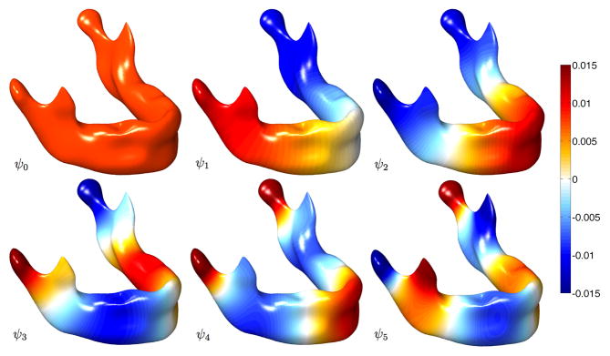
where C is the stiffness matrix, A is the mass matrix, and ψ is the unknown eigenfunction evaluated at mesh vertices. Because C and A are large sparse matrices, we have solved the problem using the Implicitly Restarted Arnoldi Method [7,9] without consuming large amount of memory and time for zero entries. The MATLAB code is given at http://brainimaging.waisman.wisc.edu/~chung/lb. Fig. 1 shows the first few eigenfunctions for a mandible surface.

Fig. 1.

The eigenfunctions are projected on the surface smoothed by the proposed heat kernel smoothing with σ = 1 and k = 139. The first eigenfunction is simply ${\psi }_0=1/\sqrt{\mu (\mathcal{M})}$. The color scale is thresholded at ±0.015 for better visualization.

Finite Eigenfunction Expansion

Let be the subspace spanned by up to k-th degree basis. Then an arbitrary measurement Y is estimated in the subspace by minimizing the sum of squared residual:

$$arg\underset{g\in {\mathcal{H}}_k}{min}{\left|\right|g-Y(p)\left|\right|}^2=\sum _{j=0}^k{\beta }_j{\psi }_j(p).$$ (7)

Consider the triangular mesh for with N_v nodes, and let β = (β₀, ···, β_k )′ and Y = (Y(p₁), ···, Y(p_Nv))′, for k ≤ N_v. Then, we can represent (7) as the normal equation,

$$\mathbf{Y}=\mathit{\beta }\mathbf{\Psi },$$ (8)

where Ψ = (Ψ₀, ···, Ψ_k) and Ψ_j = (ψ_j(p₁), ···, ψ_j(p_Nv))′, and β are estimated in the least squares fashion, β̂ = (Ψ′Ψ)⁻¹Ψ′Y. Since the size of matrix Ψ′Ψ can become fairly large when there is a need to obtain large number of basis, it may be difficult to directly invert the matrix. So we have adopted a more general iterative strategy to overcome possible computational bottleneck for large k.

Iterative Residual Fitting Algorithm

The Fourier coefficients are estimated based on an iterative procedure that utilizes the orthonormality of the eigenfunctions [2]. Decompose the subspace into smaller subspaces as the direct sum = ⊕ ··· ⊕ , where each subspace is the projection of along the j-th eigenfunction. Instead of directly solving the normal equation (8), we project the normal equations into a smaller subspace and find the corresponding β_j in an iterative fashion from increasing the degree from 0 to k.

At degree k = 0, we write Y = Ψ₀β₀+r₀, where r₀ is the residual of estimating Y in subspace . Then, we estimate β₀ by minimizing the residual in the least squares fashion:

$${\widehat{\beta }}_0={({\mathbf{\Psi }}_0^{\prime }{\mathbf{\Psi }}_0)}^{-1}{\mathbf{\Psi }}_0^{\prime }\mathbf{Y}$$ (9)

At degree j, we have

$${\mathbf{r}}_{j-1}={\mathbf{\Psi }}_j{\beta }_j+{\mathbf{r}}_j,$$ (10)

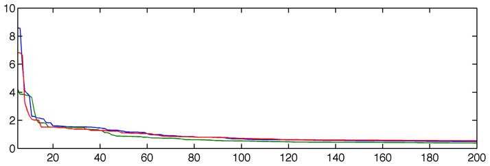
where the previous residual r_j−1 = Y − Ψ₀β̂₀ ··· −Ψ_j−1β̂_j−1. The next residual r_j is then estiamted as ${\widehat{\beta }}_j={({\mathbf{\Psi }}_j^{\prime }{\mathbf{\Psi }}_j)}^{-1}{\mathbf{\Psi }}_j^{\prime }{\mathbf{r}}_{j-1}$. The optimal stopping rule is determined if the decrease of the root mean squared errors (RMSE), $\sqrt{{\sum }_{i=1}^{N_v}{\mathbf{r}}_k^2(p_i)/N_v}$, is statistically significant using the F-test (Fig. 2). We compute the F statistic at each degree, and find the degree of expansion where corresponding p-value first becomes bigger than the pre-specified significance 0.01.

Fig. 2.

The plot of the root mean squared errors (RMSE) for coordinates x (blue), y (red) and z (green) for a sample mandible surface, varying degree k from 5 to 200. The optimal degree for the surface is determined as 139.

4 Experimental Results

We applied the proposed smoothing method to mandible surfaces obtained from CT and further compared it against iterative kernel smoothing method [3,6].

Image Acquisition and Preprocessing

The CT images were obtained using several different models of GE multi-slice helical CT scanners. The CT scans were acquired directly in the axial plane with a 1.25 mm slice thickness, matrix size of 512 × 512 and 15–30 cm FOV. Image resolution varied and was in the range of 0.29 to 0.59 mm as determined by the ratio of field of view (FOV) divided by the matrix. CT scans were converted to DICOM format and subsequently Analyze 8.1 software package (AnalyzeDirect, Inc., Overland Park, KS) was used in segmenting binary mandibular structure based on histogram thresholding. By checking the Euler characteristic, holes in mandible images were automatically filled up using morphological operations. This process was necessary to make the mandible binary volume to be topologically equivalent to a solid sphere and and produces the surface mesh that is topologically equivalent to a sphere.

Results

We applied the proposed method in smoothing a mandibular surface. The optimal eigenfunction expansion was determined using the F-test at α = 0.01. Fig. 2 shows the plot of the RMSE for varying degrees between 5 to 200. As the degree k increases, the RMSE for each coordinate rapidly decreases and starts to flatten out at a certain degree.

The numerical implementation was done with MATLAB 7.9 in 2 × 2.66 GHz Quad-Core Intel Xeon processor MAC PRO with 32 GB memory. For a mesh with 22050 vertices, the entire process took approximately 105 seconds: 85 seconds for setting up the generalized eigenvalue problem (6), 10 seconds for actually solving (6), 0.1 seconds for the IRF, and 9 seconds for finding the optimal degree.

Comparison

The proposed heat kernel smoothing was compared against widely used iterated kernel smoothing [3,6] of which the MATLAB code is given in http://www.stat.wisc.edu/mchung/softwares/hk/hk.html. In iterated kernel smoothing, the weights of the kernel are spatially adapted to follow the shape of heat kernel in discrete fashion along a surface mesh. Smoothing with large bandwidth is broken into iterated smoothing with smaller bandwidths:

$$K_{m\sigma }\ast Y=\underset{m\mathit{times}}{\underbrace{K_{\sigma }\ast \cdots \ast K_{\sigma }}}\ast Y.$$ (11)

For small σ, using the parametrix expansion [12], we can approximate heat kernel locally using the Gaussian kernel for small bandwidth:

$$K_{\sigma }(p,q)=\frac{1}{\sqrt{4\pi \sigma }}exp[-\frac{d^2(p,q)}{4\sigma }][1+O({\sigma }^2)],$$ (12)

where d(p, q) is the geodesic distance between p and q. For sufficiently small bandwidth, all the kernel weights are concentrated near the center, so the first neighbors of a given vertex in a mesh is used in the approximation.

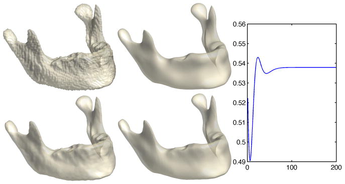
By taking the proposed heat kernel smoothing as the ground truth, we were able to determine the performance of iterated kernel smoothing. Due to the lack of the ground truth, there are no studies in the literature validating the performance of iterated kernel smoothing except [5]. For heat kernel smoothing, we used the bandwidth σ = 1 and eigenfunctions up to k = 139 degree. For iterated kernel smoothing, we varied the number of iterations 1 ≤ m ≤ 200 with the correspondingly smaller bandwidth 1/m to have the effective bandwidth of 1. The performance of the iterated kernel smoothing depended on the number of iterations, as shown in the plot of RMSE of x-coordinate over the number of iterations (Fig. 3 right). The RMSE was up to 0.5430 and it did not decrease even when we increase the number of iterations. This comparison directly demonstrates for the first time, the limitation of iterated heat kernel smoothing which does not converge to heat diffusion.

Fig. 3.

Top left: original mandible surface. Top right: heat kernel smoothing with σ = 1 and k = 139. This is taken as the ground truth and iterative kernel smoothing is compared. Bottom left: iterative kernel smoothing with σ = 1/6 and m = 6 when the reconstruction error is minimum. Bottom right: iterative kernel smoothing with σ = 1/6 and m = 30. Right: RMSE for x-coordinate over the number of iterations m.

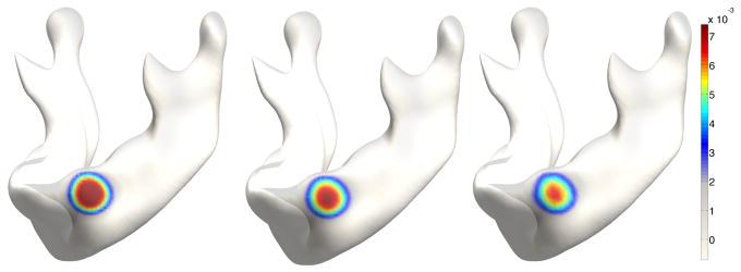
In another comparison (Fig. 4), we numerically constructed a heat kernel with a small bandwidth 0.2 as a sample data. Then we performed the additional iterated kernel smoothing with σ = 0.2 and m = 49 on the sample data to obtain the effective smoothing bandwidth of 10. The result was compared with the proposed heat kernel smoothing with the bandwidth 9.8 on the sample data making the effective bandwidth of 10. From Fig. 4, we immediately see that the shapes of two kernels are different. This visually demonstrates iterated kernel smoothing substantially diverges from heat kernel smoothing.

Fig. 4.

Comparison of the shape of kernels. Left: heat kernel with 0.2 used as a sample data. Middle: The sample data is smoothed with heat kernel smoothing method with bandwidth σ = 9.8 making the effective bandwidth of 10. Right: iterated kernel smoothing with bandwidth σ = 0.2 and m = 49 iterations applied to the sample data.

5 Conclusions

We present a novel surface data smoothing framework where a smoothed surface measure is represented as a weighted linear combination of Laplace-Beltrami eigenfunctions. The expansion analytically solves isotropic heat diffusion. Taking the expansion as the ground truth, the proposed method is compared against widely used iterated kernel smoothing. The proposed method outperforms iterated kernel smoothing in accuracy. The divergence of iterated kernel smoothing is visually represented as kernel shapes on the mandible confirming the superiority of this proposed framework.

References

- 1.Andrade A, Kherif F, Mangin J, Worsley KJ, Paradis A, Simon O, Dehaene S, Le Bihan D, Poline JB. Detection of fmri activation using cortical surface mapping. Human Brain Mapping. 2001;12:79–93. doi: 10.1002/1097-0193(200102)12:2<79::AID-HBM1005>3.0.CO;2-I. [DOI] [PMC free article] [PubMed] [Google Scholar]
- 2.Chung MK, Dalton KM, Shen L, Evans AC, Davidson RJ. Weighted Fourier representation and its application to quantifying the amount of gray matter. IEEE Transactions on Medical Imaging. 2007;26:566–581. doi: 10.1109/TMI.2007.892519. [DOI] [PubMed] [Google Scholar]
- 3.Chung MK, Robbins S, Dalton KM, Davidson RJ, Alexander AL, Evans AC. Cortical thickness analysis in autism with heat kernel smoothing. NeuroImage. 2005;25:1256–1265. doi: 10.1016/j.neuroimage.2004.12.052. [DOI] [PubMed] [Google Scholar]
- 4.Chung MK, Taylor J. Diffusion smoothing on brain surface via finite element method. Proceedings of IEEE International Symposium on Biomedical Imaging, ISBI; 2004. [Google Scholar]
- 5.Hagler AP, Jr, Saygin DJ, Sereno MI. Smoothing and cluster thresholding for cortical surface-based group analysis of FMRI data. NeuroImage. 2006;33:1093–1103. doi: 10.1016/j.neuroimage.2006.07.036. [DOI] [PMC free article] [PubMed] [Google Scholar]
- 6.Han X, Jovicich J, Salat D, van der Kouwe A, Quinn B, Czanner S, Busa E, Pacheco J, Albert M, Killiany R, et al. Reliability of MRI-derived measurements of human cerebral cortical thickness: the effects of field strength, scanner upgrade and manufacturer. Neuroimage. 2006;32:180–194. doi: 10.1016/j.neuroimage.2006.02.051. [DOI] [PubMed] [Google Scholar]
- 7.Hernandez V, Roman JE, Tomas A, Vidal V. A survey of software for sparse eigenvalue problems. Technical Report STR-6, Universidad Politécnica de Valencia. 2006 http://www.grycap.upv.es/slepc.
- 8.Joshi AA, Shattuck DW, Thompson PM, Leahy RM. A parameterization-based numerical method for isotropic and anisotropic diffusion smoothing on non-flat surfaces. IEEE Transactions on Image Processing. 2009;18(6):1358–1365. doi: 10.1109/TIP.2009.2016163. [DOI] [PMC free article] [PubMed] [Google Scholar]
- 9.Lehoucq RB, Sorensen DC, Yang C. ARPACK Users’ Guide: Solution of Large-Scale Eigenvalue Problems with Implicitly Restarted Arnoldi Methods. SIAM Publications; Philadelphia: 1998. [Google Scholar]
- 10.Lévy B. Laplace-Beltrami Eigenfunctions: Towards an Algorithm that Understands Geometry. IEEE International Conference on Shape Modeling and Applications; Los Alamitos: IEEE; 2006. p. 13. [Google Scholar]
- 11.Qiu A, Bitouk D, Miller MI. Smooth functional and structural maps on the neocortex via orthonormal bases of the laplace-beltrami operator. IEEE Transactions on Medical Imaging. 2006;25:1296–1396. doi: 10.1109/tmi.2006.882143. [DOI] [PubMed] [Google Scholar]
- 12.Rosenberg S. The Laplacian on a Riemannian Manifold. Cambridge University Press; Cambridge: 1997. [Google Scholar]
- 13.Spira A, Kimmel R, Sochen N. A short-time Beltrami kernel for smoothing images and manifolds. IEEE Transactions on Image Processing. 2007;16:1628–1636. doi: 10.1109/tip.2007.894253. [DOI] [PubMed] [Google Scholar]
- 14.Tasdizen T, Whitaker R, Burchard P, Osher S. Geometric Modeling and Processing. 2006. Geometric surface smoothing via anisotropic diffusion of normals; pp. 687–693. [Google Scholar]