Using VMD - An Introductory Tutorial

Abstract

VMD (Visual Molecular Dynamics) is a molecular visualization and analysis program designed for biological systems such as proteins, nucleic acids, lipid bilayer assemblies, etc. This unit will serve as an introductory VMD tutorial. We will present several step-by-step examples of some of VMD’s most popular features, including visualizing molecules in three dimensions with different drawing and coloring methods, rendering publication-quality figures, animate and analyze the trajectory of a molecular dynamics simulation, scripting in the text-based Tcl/Tk interface, and analyzing both sequence and structure data for proteins.

Introduction

VMD (Visual Molecular Dynamics) (Humphrey et al., 1996) is a molecular visualization and analysis program designed for biological systems such as proteins, nucleic acids, lipid bilayer assemblies, etc. It is developed by the Theoretical and Computational Biophysics Group at the University of Illinois at Urbana-Champaign. Among molecular graphics programs, VMD is unique in its ability to efficiently operate on multi-gigabyte molecular dynamics trajectories, its interoperability with a large number of molecular dynamics simulation packages, and its integration of structure and sequence information.

Key features of VMD include:

• General 3-D molecular visualization with extensive drawing and coloring methods

• Extensive atom selection syntax for choosing subsets of atoms for display

• Visualization of dynamic molecular data

• Visualization of volumetric data

• Support for most molecular data file formats

• No limits on the number of atoms, molecules, or trajectory frames, except available memory

• Molecular analysis commands

• Rendering high-resolution, publication-quality molecule images

• Movie making capability

• Building and preparing systems for molecular dynamics simulations

• Interactive molecular dynamics simulations

• Extensions to the Tcl/Python scripting languages

• Extensible source code written in C and C++

This unit will serve as an introductory VMD tutorial. It is impossible to cover all of VMD’s capabilities in one unit; instead we will present several step-by-step examples of VMD’s basic features. Topics covered in this tutorial include visualizing molecules in three dimensions with different drawing and coloring methods, rendering publication-quality figures, animating and analyzing the trajectory of a molecular dynamics simulation, scripting in the text-based Tcl/Tk interface, and analyzing both sequence and structure data for proteins.

DOWNLOADING VMD

Before staring, the current version of VMD needs to be downloaded. This tutorial was written for VMD version 1.8.6. VMD supports all major computer platforms and can be obtained from the VMD homepage http://www.ks.uiuc.edu/Research/vmd. Follow the instruction online to install. Once VMD is installed, to start VMD:

• Mac OS X: Double click on the VMD application icon in the Applications directory.

• Linux and SUN: Type vmd in a terminal window.

• Windows: Select Start → Programs → VMD.

When VMD starts, by default three windows will open: the VMD Main window, the OpenGL Display window, and the VMD Console window (or a Terminal window on a Mac). To end a VMD session, go to the VMD Main window, and choose File → Quit. You can also quit VMD by closing the VMD Console window or the VMD Main window.

TOPICS AND FILES

This unit contains six sections. Each section acts as an independent tutorial for a specific topic (Working with a Single Molecule, Trajectories and Movie Making, Scripting in VMD, Working with Multiple Molecules, Comparing Protein Structures and Sequences with the MultiSeq Plugin, and Data Analysis in VMD). For readers with no prior experience with VMD, we suggest they work through the sections in the order they are presented. Readers already familiar with the basics of VMD may selectively pursue sections of their interest. Several files have been prepared to accompany this tutorial. You need to download these files HERE.

WORKING WITH A SINGLE MOLECULE

In this section the basic functions of VMD will be introduced, starting with loading a molecule, displaying the molecule, and rendering publication-quality molecule images. This section uses the protein ubiquitin as an example molecule. Ubiquitin is a small protein responsible for labeling proteins for degradation, and is found in all eukaryotes with nearly identical sequences and structures.

Necessary Resources

Hardware

Computer

Software

VMD, and an image-displaying program

Files

1ubq.pdb, which can be downloaded

BASIC PROTOCOL 1

Loading and Displaying the Molecule

A VMD session usually starts with loading structural information of a molecule into VMD. When VMD loads a molecule, it accesses the information about the names and coordinates of the atoms. Then, one can explore various VMD visualization features to get a nice view of the loaded molecule.

Loading a Molecule

The first step is to load the molecule. The pdb file, 1ubq.pdb (Vijay-Kumar et al., 1987) that contains the atomic coordinates of ubiquitin will be loaded.

• 1. Start a VMD session. In the VMD Main window, choose File → New Molecule… (Figure 2(a)). The Molecule File Browser window (Figure 2(b)) will appear on the screen.

• 2. Use the Browse… (Figure 2(c)) button to find the file 1ubq.pdb. When file is selected, you will be back in the Molecule File Browser window. In order to actually load the file, press Load (Figure 2(d)).

• 3. Now, ubiquitin is shown in the OpenGL Display window. Close the Molecule File Browser window at any time.

  VMD can download a pdb file from the Protein Data Bank (http://www.pdb.org) if a network connection is available. Just type the four letter code of the protein in the File Name text entry of the Molecule File Browser window and press the Load button. VMD will download it automatically.

Figure 2.

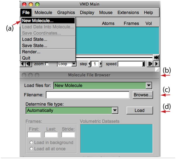
Loading a molecule.

Display the Molecule

In order to see the 3D structure of our protein, the mouse will be used in multiple modes to change the viewpoint. VMD allows users to rotate, scale and translate the viewpoint of the molecule.

• 4. In the OpenGL Display, press the left mouse button down and move the mouse. Explore what happens. This is the rotation mode of the mouse and allows for rotatation of the molecule around an axis parallel to the screen (Figure 3(a)).

• 5. Holding down the right mouse button and repeating the previous step will cause rotation around an axis perpendicular to the screen (Figure 3(b)).

  For Mac users who have a single-button mouse or a trackpad, the right mouse button is equivalent to holding down the command key while pressing the mouse/trackpad button).

• 6. In the VMD Main window, look at the Mouse menu (Figure 4). Here, the user is able to switch the mouse mode from Rotation to Translation or Scale modes.

• 7. Choose the Translation mode and go back to the OpenGL Display. It is now possible to move the molecule around when you hold the left mouse button down.

• 8. Go back to the Mouse menu and choose the Scale mode this time. This will allow the user to zoom in or out by moving the mouse horizontally while holding down the left mouse button.

  It should be noted that these actions performed with the mouse only change the viewpoint and do not change the actual coordinates of the molecule’s atoms.

  Also note that each mouse mode has its own characteristic cursor and its own shortcut key (r: Rotate, t: Translate, s: Scale). When the OpenGL Display window is the active window, these shortcut keys can be used instead of the Mouse menu to change the mouse mode.

  Another useful option is the Mouse → Center menu item. It allows you to specify the point around which rotations are done.

• 9. Select the Center menu item and pick one atom at one of the ends of the protein; the cursor should display a cross.

• 10. Now, press r, and rotate the molecule with the mouse and see how the molecule moves around the selected point.

• 11. In the VMD Main window, select the Display → Reset View menu item to return to the default view. You can also reset the view by pressing the “=” key when you are in the OpenGL Display window.

Figure 3.

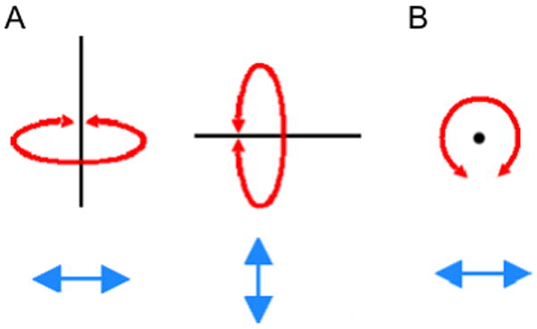
Rotational modes. (A) Rotation axes when holding down the left mouse key. (B) The rotation axes when holding down the right mouse key.

Figure 4.

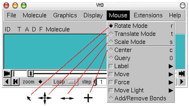
Mouse modes and their characteristic cursors.

Graphical Representations

VMD can display molecules in various ways by setting the Graphical Representations window shown in Figure 5. Each representation is defined by four main parameters: the selection of atoms included in the representation, the drawing style, the coloring method, and the material. The selection determines which part of the molecule is drawn, the drawing method defines which graphical representation is used, the coloring method gives the color of each part of the representation, and the material determines the effects of lighting, shading, and transparency on the representation. Let us first explore different drawing styles.

Figure 5.

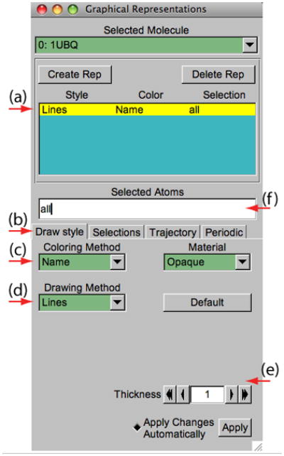
The Graphical Representations window.

Exploring different drawing styles

• 12. In the VMD Main window, choose the Graphics → Representations… menu item. A window called Graphical Representations will appear and the current default representation will be highlighted in yellow (Figure 5a).

• 13. In the Draw Style tab (Figure 5(b)) change the style (Figure 5(d)) and color (Figure 5(c)) of the representation. Here we will focus on the drawing style (the default is Lines).

• 14. Each Drawing Method has its own parameters. For instance, change the Thickness of the lines by using the controls on the lower right-hand-side corner (Figure 5(e)) of the Graphical Representations window.

• 15. Click on the Drawing Method (Figure 5(d)), to see a list of options. Choose VDW (van der Waals); each atom is now represented by a sphere scaled to its vander Waals radius, allowing the user to see the volumetric distribution of the protein.

• 16. When choosing VDW as the drawing method, two new controls will show up in the lower right-hand-side corner (Figure 5(e)). Use these controls to change the Sphere Scale to 0.5 and the Sphere Resolution to 13. Note that the higher the resolution, the slower the display of the molecule will be.

• 17. Press the Default button. This returns to the default properties of the chosen drawing method.

  Other popular representations include CPK and Licorice. In CPK, like in old chemistry ball & stick kits, each atom is represented by a sphere and each bond is represented by a thin cylinder (radius and resolution of both the sphere and the cylinder can be modified). The Licorice drawing method also represents each atom as a sphere and each bond as a cylinder, but the sphere and the cylinder have the same radii.

The previous representations visualize micromolecular details of the protein by displaying every single atom. More general structural properties can be demonstrated better by using more abstract drawing methods.

• 18. Choose the Tube style under Drawing Method, which shows the backbone of the protein. Set the Radius to 0.8. The result should be similar to Figure 6.

Figure 6.

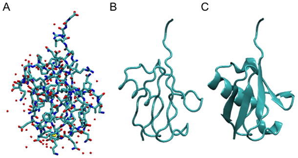
(A) Licorice, (B) Tube, and (C) NewCartoon representations of ubiquitin.

The last drawing method described here is NewCartoon. It gives a simplified representation of a protein based on its secondary structure. Helices are drawn as coiled ribbons, β-sheets as solid, flat arrows and all other structures as a tube. This is probably the most popular drawing method to view the overall architecture of a protein.

• 19. In the Graphical Representations window, choose Drawing Method → NewCartoon. The helices, β-sheets and coils of the protein can now be easily identified.

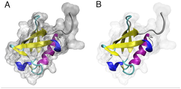
  Ubiquitin has three and one half turns of α-helix (residues 23 to 34, three of them hydrophobic), one short piece of 3₁₀-helix (residues 56 to 59) and a mixed β-sheet with five strands (residues 1 to 7, 10 to 17, 40 to 45, 48 to 50, and 64 to 72) and seven reverse turns. VMD uses the program STRIDE (Frishman and Argos, 1995) to compute the secondary structure according to a heuristic algorithm.

Exploring different coloring methods

In this series of steps, different coloring methods representations are explored.

• 20. In the Graphical Representations window, the default coloring method is Coloring Method → Name. In this coloring method, choose a drawing method that shows individual atoms: each atom will have a different color, i.e: O is red, N is blue, C is cyan and S is yellow.

• 21. Choose Coloring Method → ResType (Figure 5(c)). This allows non-polar residues (white) to be distinguished from basic residues (blue), acidic residues (red), and polar residues (green).

• 22. Select Coloring Method → Structure (Figure 5(c)) and confirm that the NewCartoon representation displays colors consistent with secondary structure.

Displaying different selections

To display only parts of the molecule of interest, one can specify their selection in the Graphical Representations window (Figure 5(f)).

• 23. In the Graphical Representations window, there is a Selected Atoms text entry (Figure 5(f)). Delete the word all, type helix and press the Apply button or hit the Enter/return key (remember to do this whenever a selection is changed!). VMD will show just the helices present in the molecule.

• 24. In the Graphical Representations window choose the Selections tab (Figure 7(a)). In section Singlewords (Figure 7(b)), a list of possible selections that can be entered is provided.

  Combinations of boolean operators can also be used when writing a selection.

• 25. In order to see the molecule without helices and β-sheets, type the following in Selected Atoms: (not helix) and (not betasheet). Remember to press the Apply button or hit the Enter/return key.

• 26. In the section Keyword (Figure 7(c)) of the Selections tab, the properties that can be used to select parts of a molecule are listed along with their possible values. Look at possible values of the keyword “resname” (Figure 7(d)).

• 27. Display all the lysines and glycines present in the protein by typing (resname LYS) or (resname GLY) in the Selected Atoms.

  Lysines play a fundamental role in the configuration of polyubiquitin chains.

• 28. Change the current representation’s Drawing Method to CPK and the Coloring Method to ResName in the Draw Style tab. In the screen, the different lysines and glycines will be visible.

• 29. In the Selected Atoms text entry type water. Choose Coloring Method → Name. The 58 water molecules present in the system show now appear (in fact only their oxygen atoms).

• 30. In order to see which water molecules are closer to the protein, use the command within. Type water and within 3 of protein for Selected Atoms. This selects all the water molecules that are within a distance of 3 Å of the protein.

• 31. Finally, try typing in Selected Atoms the selections shown in the first column of Table 1. Each of these selections will show the protein or part of the protein as expained in the second column of Table 1.

Figure 7.

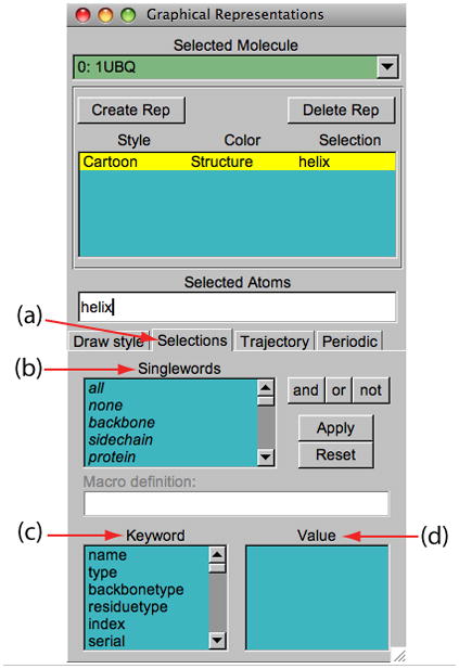
Graphical Representations window and the Selections tab.

Table 1.

Examples of atom selections.

Selection	Action
Protein	Shows the protein
resid 1	The first residue
(resid 1 76) and (not water)	The first and last residues
(resid 23 to 34) and (protein)	The α-helix

Creating multiple representations

The button Create Rep (Figure 8(a)) in the Graphical Representations window allows creation of multiple representations. Therefore, users can have a mixture of different selections with different styles and colors, all displayed at the same time.

Figure 8.

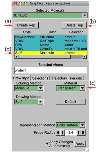
Multiple Representations of ubiquitin.

• 32. For the current representation, in Selected Atoms type protein, set the Drawing Method to NewCartoon and the Coloring Method to Structure.

• 33. Press the Create Rep button (Figure 8(a)). A new representation will be created.

• 34. Modify the new representation to get VDW as the Drawing Method, ResType as the Coloring Method, and resname LYS as the current selection.

• 35. Repeating the previous procedure, create the following two new representations in Table 2. These two representations show water molecules and the Cα atoms of the first and last residues of the protein.

• 36. Create the last representation by pressing again the Create Rep button. Select Drawing Method → Surf for drawing method, Coloring Method → Molecule for coloring method, and type protein in the Selected Atoms entry. For this last representation choose Transparent in the Material pull-down menu (Figure 8(c)). This representation shows protein’s volumetric surface in transparent.

  Note that you can select and modify different representations you have created by clicking on a representation to highlight it in yellow. Also, each representation can be switched on/off by double-clicking on it. To delete a representation, highlight it and then click on the Delete Rep button (Figure 8(b)). At the end of this section, the Graphical Representations window should look like Figure 8.

Table 2.

Examples of representations.

Selection	Coloring Method	Drawing Method
Water	Name	CPK
resid 1 76 and name CA	ColorID → 1	VDW

Sequence Viewer Extension

When dealing with a protein for the first time, it is very useful to be able to find and display different amino acids quickly. The sequence viewer extension allows viewing of the protein sequence, as well as to easily pick and display one or more residues of interest.

• 37. In the VMD Main window, choose the Extension → Analysis → Sequence Viewer menu item. A window (Figure 9(a)) with a list of the amino acids (Figure 9(e)) and their properties (Figures 9(b)&(c)) will appear on the screen.

• 38. With the mouse, try clicking on different residues in the list (Figure 9(e)) and see how they are highlighted. In addition, the highlighted residue will appear in the OpenGL Display window in yellow and rendered in the bond drawing method, so its location within the protein can be visualized easily.

• 39. Use the Zoom controls (Figure 9(f)) to display the entire list of residues in the window. This is particularly useful for larger proteins.

• 40. Pick multiple residues by holding the shift key and clicking on the mouse button (Figure 9(e)).

• 41. Look at the Graphical Representations window, a new representation with the residues that have been selected using the Sequence Viewer Extension should be shown. Modify, hide or delete this representation similar to the steps described above.

  Information about residues is color-coded (Figure 9(d)) in columns and obtained from STRIDE. The “B-value” column (Figure 9(b)) shows the B-value field (temperature factor) often provided in pdb files. The struct column shows secondary structure (Figure 9(d)), where each letter corresponds to a secondary structure, listed in Table 3.

Figure 9.

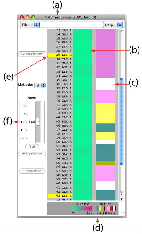
VMD Sequence window.

Table 3.

Secondary Structure codes used by STRIDE.

Letter Code	Secondary Structure
T	Turn
E	Extended conformation (β-sheets)
B	Isolated bridge
H	Alpha helix
G	3–10 helix
I	Pi helix
C	Coil

Saving Your Work

The viewpoints and representations created using VMD can be saved as a VMD state. This VMD state contains all the information needed to reproduce the same VMD session.

• 42. Go to the OpenGL Display window, use the mouse to find a nice view of the protein. We will save this viewpoint using the VMD ViewMaster.

• 43. In the VMD Main window, select Extension → Visualization → ViewMaster. This will open the VMD ViewMaster window.

• 44. In the VMD ViewMaster window, click on the Create New button. The OpenGL Display viewpoint has now been saved.

• 45. Go back to the OpenGL Display window and use the mouse to find another nice view. If desired, add/delete/modify a representation in the Graphical Representations window. When a good view has been found, save it by returning to the VMD ViewMaster window and clicking on the Create New button.

• 46. Create as many views as desired by repeating the previous step. All of viewpoints are displayed as thumbnails in the VMD ViewMaster window. A previously-saved viewpoint can be opened by clicking on its thumbnail.

• 47. To save the entire VMD session, in the VMD Main window, choose the File → Save State menu item. Write an appropriate name (e.g., myfirststate.vmd) and save it.

  The VMD state file myfirststate.vmd contains all the information needed to restore a VMD session, including the viewpoints and the representations.

  To load a saved VMD state, start a new VMD session and in the VMD Main window choose File → Load State.

• 48. Quit VMD.

Basic Protocol 2

The Basics of VMD Figure Rendering

One of VMD’s many strengths is its ability to render high-resolution, publication-quality molecule images. In this section we will introduce some basic concepts of figure rendering in VMD.

Setting the display background

Before rendering a figure, make sure that the OpenGL Display background is set up the way you want. Nearly all aspects of the OpenGL Display are user-adjustable, including the background color.

• 1. Start a new VMD session (Basic Protocol 1) and load the 1ubq.pdb file.

• 2. In the VMD Main window, choose Graphics → Colors…. The Color Controls window should show up. Look through the Categories list. All display colors, for example, the colors of different atoms when colored by name, are set here.

• 3. In Categories, select Display. In Names, select Background. Finally, choose “8 white” in Colors. The OpenGL Display now should have a white background.

• 4. When making a figure, we often do not want to include the axes. To turn of the axes, select Display → Axes → Off in the VMD Main window.

Increasing geometric resolution

All VMD objects are drawn with an adjustable resolution, allowing users to balance fineness of detail with drawing speed.

• 5. Open the Graphical Representation window via Graphics → Representations… in the VMD Main menu. Modify the default representation to show just the protein, and display it using the VDW drawing method.

• 6. Zoom in on one or two of the atoms by using Mouse → Scale Mode (shortcut s).

  You might notice that as you zoom into an atom closer and closer, the atom might be cut off by an invisible clipping plane, which makes it difficult to focus on just one atom. This is an OpenGL feature. You can move the clipping plane closer to you by doing the following: switch your mouse mode to the Translate mode, either by pressing the shortcut key “t” in the OpenGL window or by selecting Mouse → Translate Mode, and drag your mouse in the OpenGL window while holding down the right mouse key. You can now move the clipping plane closer to you, or away from you. If this does not work, here is an alternative way: in the VMD Main window, choose Display → Display Settings…; in the Display Settings window that shows up, Many OpenGL options are adjustable; decrease the value for Near Clip, which will move the OpenGL clipping closer, allowing you to zoom in on individual atoms without clipping them off.

• 7. Notice that with the default resolution setting, the “spherical” atoms are not looking very spherical. In the Graphical Representations window, click on the representation you set up before for the protein to highlight it in yellow. Try adjusting the Sphere Resolution setting to something higher, and see what a difference it can make (Figure 10).

  Most of the drawing methods have a geometric resolution setting. Try a few different drawing methods and see how their resolutions can be easily increased. When producing images, the resolution can be raised until it stops making a visible difference.

Figure 10.

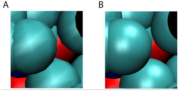
The effect of the resolution setting. (A) Low resolution: Sphere Resolution set to 8. (B) High resolution: Sphere Resolution set to 28.

Colors and materials

• 8. There is a Material menu in the Graphical Representations window (which by default is set to Opaque material). Choose the protein representation you made before, and experiment with the different materials in the Material menu.

• 9. Besides the pre-defined materials in the Material menu, VMD also allows users to create their own materials. To make a new material, in the VMD Main window choose Graphics → Materials….

• 10. In the Materials window that appears, you will see a list of the materials you just tried out, and their adjustable settings. Click the Create New button. A new material, Material 12, will be created. Give it the settings listed in Table 4.

• 11. Go back to the Graphical Representations window. In the Material menu, Material 12 is now on the list. Try using Material 12 for a representation and see what it looks like. You can also rename the materials in the Material menu.

  Now is a good time to try out the GLSL Render Mode, if your computer supports it. In the VMD Main window, choose Display → Rendermode → GLSL. This mode uses your 3D graphics card to render the scene with real-time ray-tracing of spheres and alpha-blended transparency, and can improve the visualization of transparent materials. See Figure 11 for example renderings made in GLSL mode.

• 12. If your computer supports GLSL Render Mode, you can try to reproduce Figure 11. First turn on the GLSL rendering mode by selecting Display → Rendermode → GLSL in the VMD Main window.

• 13. Modify Material 12 to be more transparent by entering the values listed in Table 5 in the Materials window.

• 14. Hide all of the current representations and create the two representations in Table 6.

Table 4.

Example of a user-defined material.

Setting	Value
Ambient	0.30
Diffuse	0.30
Specular	0.90
Shininess	0.50
Opacity	0.95

Figure 11.

Examples of different material settings. (A) The default transparent material, rendered in GLSL mode. (B) A user-defined material with high transparency, also rendered in GLSG mode.

Table 5.

Example of a more transparent material.

Setting	Value
Ambient	0.30
Diffuse	0.50
Specular	0.87
Shininess	0.85
Opacity	0.11

Table 6.

Example of representations drawn with different materials.

Selection	Coloring Method	Drawing Method	Material
protein	Structure	NewCartoon	Opaque
protein	ColorID→8 white	Surf	Material 12

Depth perception

Since the molecular systems are three-dimensional, VMD has multiple ways of representing the third dimension. In this section, how to use VMD to enhance or hide depth perception is discussed.

• 15. The first thing to consider is the projection mode. In the VMD Main window, click the Display menu. Here we can choose either Perspective or Orthographic in the drop-down menu. Try switching between Perspective or Orthographic projection modes and see the difference (Figure 12).

  In perspective mode, things nearer the camera appear larger. Perspective projection provides strong size-based visual depth cues, but the displayed image will not preserve scale relationships or parallelism of lines, and objects very close to the camera may appear distorted. Orthographic projection preserves scale and parallelism relationships between objects in the displayed image, but greatly reduces depth perception. Hence, orthographic mode tends to be more useful for analysis, because alignment is easy to see, while perspective mode is often used for producing figures and stereo images.

  Another way VMD can represent depth is through so-called “depth cueing”. Depth cueing is used to enhance three-dimensional perception of molecular structures, particularly with orthographic projections.

• 16. Choose Display → Depth Cueing in the VMD Main window.

  When depth cueing is enabled, objects further from the camera are blended into the background. Depth cueing settings are found in Display → Display Settings…. Here one can choose the functional dependence of the shading on distance, as well as some parameters for this function. To see the depth cueing effect better, you might want to hide the representation with the Surf drawing method.

• 17. Finally, VMD can also produce stereo images. In the VMD Main window, look at the Display → Stereo menu, showing many different choices. Choose SideBySide (remember to return to Perspective mode for a better result). The result should look like Figure 13.

• 18. Turn off stereo image by selecting Display → Stereo → Off in the VMD Main window. Also turn off depth cueing by unselecting the Display → Depth Cueing checkbox in the VMD Main window.

Figure 12.

Comparison of the (A) perspective and (B) orthographic projection modes.

Figure 13.

Stereo image of the ubiquitin protein. Shown here with Cue Mode = Linear, Cue Start = 1.5, and Cue End = 2.75.

Rendering

By now we have seen some techniques for producing nice views and representaions of the molecule loaded in VMD. Now, we will explore the use of the VMD built-in snapshot feature and external rendering programs to produce high quality images of your molecule. The “snapshot” renderer saves the on-screen image in the OpenGL window and is adequate for use in presentations, movies, and small figures. When one desires higher quality images, renderers such as Tachyon and POV-Ray are better choices.

• 19. Hide or delete all previous representations, and create the four new representations listed in Table 7.

• 20. Once you have the scene set the way you like it in the OpenGL window, simply choose File → Render… in the VMD Main window. The File Render Controls window will appear on the screen.

• 21. The File Render Controls allows you to choose which renderer you want to use and the file name for your image. Select “snapshot” for the rendering method, type in a filename of your choice, and click Start Rendering.

• 22. If you are using a Mac or a Linux machine, an image-processing application might open automatically that shows you the molecule you have just rendered using Snapshot. If this is not the case, use any image-processing application to take a look at the image file. Close the application when you are done to continue using VMD.

  The snapshot renderer saves exactly what is showing in your OpenGL display window—in fact, if another window overlaps the display window, it may distort the overlapped region of the image.

• 23. Try to render again using different rendering methods, particularly TachyonInternal and POV3. Compare the quality of the images created by different renderers.

  The other renderers (e.g. POV3 and Tachyon) reprocess everything, so it may not look exactly as it does in the OpenGL window. In particular, they do not “clip”, or hide, objects very near the camera. If you select Display → Display Settings… in the VMD Main window, you can set Near Clip to 0.01 to get a better idea of what will appear in your rendering.

• 24. Quit VMD.

Table 7.

Example representations.

Selection	Coloring Method	Drawing Style	Material
protein and not resid 72 to 76	Structure	NewCartoon	Opaque
protein and helix and name CA	ColorID→8	Surf	Material 12
resname GLY and not resid 72 to 76	ColorID→7	VDW	Opaque
resname LYS	ColorID→18	Licorice	Opaque

WORKING WITH TRAJECTORIES AND MAKING MOVIES

Time evolving coordinates of a system are called trajectories. They are most commonly obtained from simulations of molecular systems, but can also be generated by other means and for different purposes. Upon loading a trajectory into VMD, one can see a movie of how the system evolves in time and analyze various features throughout the trajectory. This section will introduce the basics of working with trajectory data in VMD. You will also learn how to analyze trajectory data in Basic Protocols 14, 15, and 16.

Necessary Resources

Hardware

Computer

Software

VMD, and a movie player program

Files

ubiquitin.psf and pulling.dcd, which can be downloaded from

Basic Protocol 3

Working with Trajectories

Trajectory files are commonly binary files that contain several sets of coordinates for the system. Each set of coordinates corresponds to one frame in time. An example of a trajectory file is a DCD file generated by the molecular dynamics program NAMD (Phillips et al., 2005).

Loading Trajectories

Trajectory files do not contain information of the system contained in the protein structure files (PSF). Therefore we first need to load the PSF file, and then add the trajectory data to this file.

• 1. Start a new VMD session. In the VMD Main window, select File → New Molecule…. The Molecule File Browser window will appear on your screen.

• 2. Use the Browse… button to find the file ubiquitin.psf. When you select this file, you will be back in the Molecule File Browser window. Press the Load button to load the molecule.

• 3. In the Molecule File Browser window, make sure that ubiquitin.psf is selected in the “Load files for:” pull-down menu on top, and click on the Browse button. Browse for pulling.dcd. Note the options available in the Molecule File Browser window: one can load trajectories starting and finishing at chosen frames, and adjust the stride between the loaded frames. Leave the default settings so that the whole trajectory is loaded.

• 4. Click on the Load button in the Molecule File Browser window.

  You will be able to see the frames as they are loaded into the molecule in the OpenGL window. After the trajectory finishes loading, you will be looking at the last frame of your trajectory. To go to the beginning, use the animation tools at the lower part of the VMD Main menu (see Figure 15).

• 5. Close the Molecule File Browser window.

• 6. For a convenient visualization of the protein, choose Graphics → Representations in the VMD Main menu. In the Selected Atoms field, type protein and hit Enter on your keyboard; in the Drawing Method, select NewCartoon; in the Coloring Method, select Structure.

  The trajectory you just loaded is a simulation of an AFM (Atomic Force Microscopy) experiment pulling on a single ubiquitin molecule, performed using the Steered Molecular Dynamics (SMD) method (Isralewitz et al., 2001). We are looking at the behavior of the protein as it unfolds while being pulled from one end, with the other end constrained to its original position. Each frame corresponds to 10ps of simulation time. Ubiquitin has many functions in the cell, and it is currently believed that some of these functions depend on the protein’s elastic properties, which can be probed in AFM pulling experiments. Such elastic properties are usually due to hydrogen bonding between residues in β strands of the protein molecules.

Figure 15.

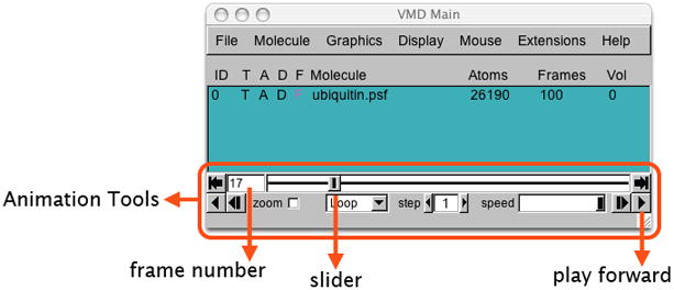
Animation tools in the VMD main menu. The tools allow one to go over frames of the trajectory (e.g., using the “slider”) and to play a movie of the trajectory in various modes (Once, Loop, or Rock) and at an adjustable speed.

Main Menu Animation Tools

You can now play the movie of the loaded trajectory back and forth, using the animation tools in Figure 15.

• 7. By dragging the slider one navigates through the trajectory. The buttons to the left and to the right from the slider panel allow one to jump to the end of the trajectory or go back to the beginning.

• 8. For example, create another representation for water in the Graphical Representations window: click on the Create Rep button; for the Selected Atoms field, type water and hit enter; for Drawing Method, choose Lines; for Coloring Method, select Name.

  This representation of water shows the water droplet present in the simulation. Using the slider, observe the behavior of the water around the protein. The shape of the water droplet changes throughout the simulation, because water molecules follow the protein as it unfolds, driven by the interactions with the protein surface.

  When playing animations, you can choose between three looping styles: Once, Loop and Rock. You can also jump to a frame in the trajectory by entering the frame number in the window on the left of the “slider” panel.

Smoothing trajectories

• 9. For clarity, turn off the water representation by double-clicking on it in the Graphical Representations window.

  As you might have noticed, when we play the animation, the protein movements are not very smooth due to thermal fluctuations (as the simulation is performed under the conditions that mimic a thermal bath). VMD can smooth the animation by averaging over a given number of frames.

• 10. In the Graphical Representations window, select your protein representation and click on the Trajectory tab. At the bottom, you should see Trajectory Smoothing Window Size set to zero. As your animation is playing, increase this setting. Notice that the motion gets smoother and smoother as the size of the smoothing window is increased. Commonly used values for this setting are 1 to 5, depending on how smooth you want your trajectory to be.

Displaying multiple frames

We will now learn how to display many frames of the same trajectory at once.

• 11. In the Graphical Representations window, highlight your protein representation by clicking on it and press the Create Rep button. This creates an identical representation, but note that smoothing is set to zero. Hide the old protein representation.

• 12. Highlight the new protein representation and click the Trajectory tab. Above the smoothing control, notice the Draw Multiple Frames control. It is set to now by default, which is simply the current frame. Enter 0:10:99, which selects every tenth frame from the range 0 to 99.

• 13. Go back to the Draw style tab, and change the Coloring Method to Timestep. This will draw the beginning of the trajectory in red, the middle in white, and the end in blue.

• 14. We can also use smoothing to make the large-scale motion of the protein more apparent. Go back to the Trajectory tab, set the smoothing window to 20. The result should look like Figure 16.

Figure 16.

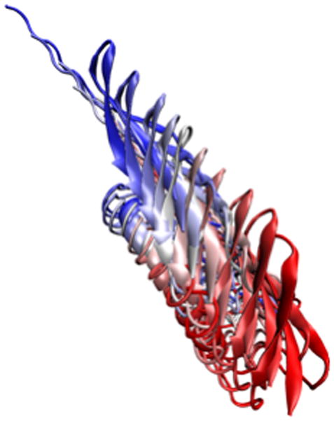
Image of every tenth frame shown at once, smoothed with a 20-frame window.

Updating selections

• 15. Now we will see how to make VMD update the selection each frame.

• 16. Hide the current representation showing all frames, and display only the water representation by double-clicking on it. Change the text in the Selected Atoms from water to water and within 3 of protein and hit enter. This will show all water atoms within 3Å of the protein.

• 17. Play the trajectory.

  As you can see, although the displayed water atoms may be near the protein for a little while, they soon wander off, and are still shown despite no longer meeting the selection criteria. The Update Selection Every Frame option in the Trajectory tab of the Graphical Representations window remedies this. If the option box is checked, the selection is updated every frame. See Figure 17.

• 18. Quit VMD.

Figure 17.

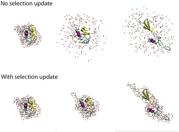
Water within 3A of the protein, shown for a selection that is not updated and for the one that is updated each frame. The snapshots shown are (from left to right) for frames 0, 17, and 99.

Basic Protocol 4

The Basics of Movie Making in VMD

The following protocol describes how to make a movie in VMD.

• 1. Start a new VMD session. Repeat steps 1–5 in Basic Protocol 2 to load the ubiquitin trajectory into VMD and display the protein in a secondary structure representation.

• 2. To make movies, we will use the VMD Movie Maker plugin. In the VMD Main window, go to menu item Extension → Visualization → Movie Maker. The VMD Movie Generator window will appear.

Making single-frame movies

• 3. Click on the Movie Settings menu in the VMD Movie Generator window, take a look at the options.

  You can see that in addiiton to a trajectory movie, Movie Maker can also make a movie by rotating the view point of a single frame. In the Renderer menu, one can choose the type of renderer for making the movie. While renderers other than Snapshot, e.g., Tachyon, generally provide more visually appealing images, they also take longer to render. The rendering time is also affected by the size of the OpenGL window, since it takes more computing time to render a larger image. We will first make a movie of just one frame of the trajectory. Here we will use the default option, Snapshot. One can also choose the output file format for the movie in menu item Format.

• 4. Select the Rock and Roll option in the Movie Settings menu in the VMD Movie Generator window. Set the working directory to any convenient directory of your choice, give your movie a name, and click Make Movie.

• 5. Once rendering is finished, open and view the movie with your favorite application. This movie setting is good for showing one side of your system primarily.

  If you cannot successfully make movies with VMD, it is possible that you are missing some software required for generating movies. All of the required softwares are freely available, and to find what software you need, please see the VMD Movie Plugin page at http://www.ks.uiuc.edu/Research/vmd/plugins/vmdmovie/

Making trajectory movies

• 6. Now we will make a movie of the trajectory. In the VMD Movie Generator window, select Movie Settings → Trajectory, give this one a different name, and click Make Movie.

  Note that the length of the movie is automatically set 24 frames per second. For a trajectory, duration of the movie can be decreased, but cannot be increased

• 7. Try out different options in the VMD Movie Generator window. Once you are done, quit VMD.

SCRIPTING IN VMD

VMD provides embedded scripting languages (Python and Tcl) for the purpose of user extensibility. In this section we will discuss the basic features of the Tcl scripting interface in VMD. You will see that everything you can do in VMD interactively can also be done with Tcl commands and scripts. We will also demonstrate how the extensive list of Tcl text commands can help you investigate molecule properties and perform various types of analysis.

Necessary Resources

Hardware

Computer

Software

VMD, and a text editor

Files

1ubq.pdb and beta.tcl, which can be downloaded from

BASIC PROTOCOL 5

The Basics of Tcl Scripting

Tcl is a rich language that contains many features and commands, in addition to the typical conditional and looping expressions. Tk is an extension to Tcl that permits the writing of graphical user interfaces with windows and buttons, etc. More information and documentations about the Tcl/Tk language can be found at http://www.tcl.tk/doc. Let us start with the basic commands.

• 1. Start a new VMD session. In the VMD Main menu select Extensions → Tk Console to open the VMD TkConsole window. You can now start entering Tcl/Tk commands here.

• 2. Try entering the following commands in the VMD TkConsole window. Remember to hit enter after each line and take a look at what you get after each input.

  set x 10
  puts “the value of x is: $x”
  set text “some text”
  puts “the value of text is: $text”
  

  As you can see, the Tcl set and put commands have the following syntax:

  • set variable value -- sets the value of variable
  • puts $variable -- prints out the value of variable

  Also, $variable refers to the value of variable.

• 3. Try the expr command by entering the following lines in the VMD TkConsole window:

  expr 3 - 8
  set x 10
  expr -3 * $x
  

  The expr command performs mathematical operations:

  • expr expression -- evaluates a mathematical expression

• 4. Entering the following example in the VMD TkConsole window:

  set result [expr -3 * $x]
  puts $result
  

  By using brackets, you can embed Tcl commands into others. A bracketed expression will automatically be substituted by the return value of the expression inside the brackets:

  • [expression]-- represents the result of the expression inside the brackets

• 5. Let us calculate the values of −3*x for integers x from 0 to 10 and output the results into a file named myoutput.dat.

  set file [open “myoutput.dat” w]
  for {set x 0} {$x <= 10} {incr x} {
  puts $file [expr -3 * $x]
  }
  close $file
  

  Here you have tried the loop feature of Tcl. Tcl provides an iterated loop similar to the “for” loop in C. The for command in Tcl requires four arguments: an initialization, a test, an increment, and the block of code to evaluate. The syntax of the “for” command is:

  • for{initialization} {test} {increment} {commands}

  Take a look at the output file myoutput.dat, either by a text editor of your choice, or the command “less” in a terminal window on a Mac or Linux Machine.

Basic Protocol 6

Working with a Molecule Using Tcl Text Commands

Anything that can be done in the VMD graphical interface can also be done with text commands. This allows scripts to be written that can automatically load molecules, create representations, analyze data, make movies, etc. Here, we will go through some simple examples of what can be done using the scripting interface in VMD.

Loading molecules with text commands

• 1. In the VMD TkConsole window, type the command mol new 1ubq.pdb and hit enter.

  As you can see, this command performs the same function as described at the beginning of Basic Protocol 1, namely, loading a new molecule with file name 1ubq.pdb.

  If you see the error message ”Unable to load file ‘1ubq.pdb’ using file type ‘pdb’”, you might not be in the correct directory that contains the file 1ubq.pdb. You can use the standard Unix commands in the VMD TkConsole window to navigate to the correct directory.

  When you open VMD, by default a vmd console window appears. The vmd console window tells you what’s going on within the VMD session that you are working on. Take a look at the vmd console window. It should tell you a molecule has been loaded, as well as some of its basic properties like number of atoms, bonds, residues and etc. The Tcl commands that you enter in the VMD TkConsole window can also be entered in the vmd console window. If you are using a Mac, your vmd console window is the terminal window that shows up when you open VMD.

Working with specific parts of a molecule: the atomselect command

Many times you might want to perform operations on only a specific part a molecule. For this purpose, VMD’s atomselect command is very useful. The atomselect command has the following syntax:

• atomselect molid “selection command”-- creates a new atom selection that includes all atoms described by “selection command”

• 2. Type set crystal [atomselect top “all”] in the Tk Console window.

  This command allows you to select a specific part of a molecule. The first argument to atomselect is the molecule ID (shown to the very left of the VMD Main window), the second argument is a textual atom selection like what you have been using to describe graphical representations in Basic Protocol 1. The selection returned by atomselect is itself a command you will learn to use.

  This step creates a selection, crystal, that contains all the atoms in the molecule and assigns it to the variable crystal. Instead of a molecule ID (which is a number), we have used the shortcut “top” to refer to the top molecule. A top molecule means that it is the target for scripting commands. This concept is particularly important when multiple molecules are loaded at the same time (see Basic Protocol 9 for dealing with multiple molecules in VMD).

  The result of atomselect is a function. Thus, $crystal is now a function that performs actions on the contents of the “all” selection.

Obtaining and changing molecule properties with text commands

After you have defined an atom selection, you have many commands that you can use to operate on it. For example, you can use commands to learn about the properties of your atom selection (number of atoms, coordinates, total charge, etc). You can also use commands to change its coordinates and other properties. See VMD User’s Guide (http://www.ks.uiuc.edu/Research/vmd/vmd-1.8.6/ug/) for an extensive list of commands.

• 3. Type $crystal num in the Tk Console window.

  Passing num to an atom selection returns the number of atoms in that selection. Check that this number matches the number of atoms for your molecule displayed in the VMD Main window.

• 4. We can also use commands to move our molecule on the screen. You can use these commands to change atom coordinates.

  $crystal moveby {10 0 0}
  $crystal move [transaxis x 40 degree]
  

Editing properties of selected atoms

• 5. Open the Graphical Representation window by selecting Graphics → Representations… in the VMD Main window. Type in protein as the atom selection, change its Coloring Method to Beta and its Drawing Method to VDW. Your molecule should now appear as a mostly red and blue assembly of spheres.

  The “B” field of a PDB file typically stores the “temperature factor” for a crystal structure and is read into VMD’s “Beta” field. Since we are not currently interested in this information, we can use this field to store our own numerical values. VMD has a “Beta” coloring method, which colors atoms according to their B-factors. By replacing the Beta values for various atoms, you can control the color in which they are drawn. This is very useful when you want to show a property of the system that you have computed.

• 6. Return to the Tk Console window and type $crystal set beta 0.

  This resets the “beta” field (which is displayed) to zero for all atoms. As you do this, you should observe that the atoms in your OpenGL window will suddenly change to a uniform color (since they all have the same beta values now).

  You can obtain and set many atomic properties using atom selections, including segment, chain, residue, atom name, position (x, y and z), charge, mass, occupancy and radius, just to name a few.

• 7. In the Tk Console window, type set sel [atomselect top “hydrophobic”].

  This creates a selection, sel, that contains all the atoms in the hydrophobic residues.

• 8. Let us label all hydrophobic atoms by setting their beta values to 1: type $sel set beta 1 in the Tk Console window. If the colors in the OpenGL Display do not get updated, go to the Graphical Representations window and click on the Apply button at the bottom.

• 9. You will now change a physical property of the atoms to further illustrate the distribution of hydrophobic residues. In the Tk Console window type $crystal set radius 1.0 to make all the atoms smaller and easier to see through, and then $sel set radius 1.5 to make atoms in the hydrophobic residues larger. The radius field affects the way that some representations (e.g., VDW, CPK) are drawn.

  You have now created a visual state that clearly distinguishes which parts of the protein are hydrophobic and which are hydrophilic. If you have followed the instructions correctly, your protein should resemble Figure 18.

  Many times in studies of proteins it is important to identify the locations of the hydrophobic residues, as they often have a functional implication. The method you have just learned is useful in this task. For example, you can see easily that in ubiquitin, the hydrophobic residues are almost exclusively contained in the inner core of the protein. This is a typical feature for small water-soluble proteins. As the protein folds, the hydrophilic residues will have a tendency to stay at the water interface, while the hydrophobic residues are pushed together and play a structural role. This helps the protein achieve proper folding and increases its stability.

Figure 18.

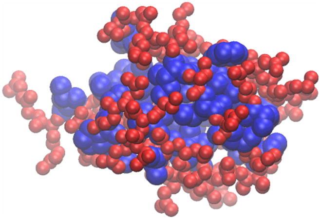
Ubiquitin in the VDW representation, colored according to the hydrophobicity of its residues.

The get command

Atom selections are useful not only for setting atomic data, but also for getting atomic information. For example, if you wish to communicate which residues are hydrophobic, all you need to do is to create a hydrophobic selection and use the get command.

• 10. Try to use the get command with your sel atom selection to obtain the names of hydrophobic residues:

  $sel get resname
  

  But there is a problem. Each residue contains many atoms, resulting in multiple repeated entries. One way to circumvent this is to pick only the α-carbons in the selection.

• 11. Type the following in the Tk Console window (note, name CA= α-carbons):

  set sel [atomselect top “hydrophobic and name CA”]
  $sel get resname
  

  This should give you the list of hydrophobic residues.

• 12. You can also get multiple properties simultaneously. Try the following:

  $sel get resid
  $sel get {resname resid}
  $sel get {x y z}
  

  If you want to obtain some of the structural properties, e.g., the geometric center or the size of a selection, the command measure can do the job easily.

• 13. Let us try using measurewith the sel selection:

  measure center $sel
  measure minmax $sel
  

  The first command above returns the geometric center of atoms in sel. And the second command returns two vectors, the first containing the minimum x, y, and z coordinates of all atoms in sel, and the second containing the corresponding maxima.

  Once you are done with a selection, it is always a good idea to delete it to save memory:

  $sel delete
  

Basic Protocol 7

Sourcing Scripts

When performing a task that requires many lines of commands, instead of typing each line in the Tk Console window, it is usually more convenient to write all the lines into a script file and load it into VMD. This is very easy to do. Just use any text editor to write your script file, and in a VMD session, use the command source filename to execute the file. You should have downloaded a simple script, beta.tcl, with this unit. We will execute it in VMD as an example. The script beta.tcl sets the colors of residues LYS and GLY to a different color from the rest of the protein by assigning them a different beta value, a trick you have already learned in Basic Protocol 6, steps 5–9.

In the Tk Console window, type sourcebeta.tcl and observe the color change. You should see that the protein is mostly a collection of red spheres, with some residues shown in blue. The blue residues are the LYS and GLY residues in the ubiquitin. Take a quick look at the script beta.tcl. Using any text editor of your choice, open the file beta.tcl. There are six lines in this file, and each line represents a Tcl command line that you have used before. Close the text editor when you are done.

The .vmd file you saved in Basic Protocol 1, step 47, is actually a series of commands. You are encouraged to take a look at that file using a text editor. Hopefully, by the end of this section, you’ll understand many of those commands. In fact, you can execute the file in the Tk Console the same way as you execute other script files, i.e., by typing source myfirststate.vmd in the Tk Console window.

Many times when you write a script you might want to look up the command for an interactive VMD feature. You can either find it in the VMD User’s Guide (http://www.ks.uiuc.edu/Research/vmd/vmd-1.8.6/ug/), or conveniently use the console command. Try typing logfile console in your Console window. This creates a logfile for all your actions in VMD and writes them in the Console window as command lines. If you execute those command lines you can repeat the exact same actions you have performed interactively. To turn off logfile, type logfile off.

Basic Protocol 8

Drawing Shapes Using VMD Text Commands

VMD offers a way to display user-defined objects built from graphics primitives such as points, lines, cylinders, cones, spheres, triangles, and text. The command that can realize those functions is graphics, the syntax of which is graphics molid command, where molid is a valid molecule ID and command is one of the commands shown below. Let us try drawing some shapes with the following examples.

• 1. Hide all representations in the Graphics Representations window.

• 2. Let us draw a point. Type the following command in your Tk Console window:

  graphics top point {0 0 10}
  

  Somewhere in your OpenGL window there should be a small dot.

• 3. Let us draw a line. Type the following command in your Console window:

  graphics top line {−10 0 0} {0 0 0} width 5 style solid
  

  This will give you a solid line.

• 4. You can also draw a dashed line:

  graphics top line {10 0 0} {0 0 0} width 5 style dashed
  

  All the objects so far are all drawn in blue. You can change the color of the next graphics object by using the command graphics top colorcolorid. The colorid for each color can be found in Graphics → Colors… menu in VMD Main window. For example, the color for orange is “3”.

• 5. Type graphics top color 3 in the Tk Console window, and the next object you draw will appear in orange.

• 6. Try the following commands to draw more shapes (note the “\” in command line means the next line is a continuation of the previous line, hence do not actually type “\” when you enter the following command, and do not start a new line):

  graphics top cylinder {5 0 0} {15 0 10} radius 10 resolution\ 60 filled no
  graphics top cylinder {0 0 0} {−5 0 10} radius 5 resolution\ 60 filled yes
  graphics top cone {40 0 0} {40 0 10} radius 10 resolution 60
  graphics top triangle {80 0 0} {85 0 10} {90 0 0}
  graphics top text {40 0 20} “my drawing objects”
  

• 7. In your OpenGL window, there are a lot of objects now. To find the list of objects you’ve drawn, use the command graphics top list. You’ll get a list of numbers, standing for the ID of each object.

• 8. The detailed information about each object can be obtained by typing graphics top info ID. For example, type graphics top info 0 to see the information on the point you drew.

• 9. You can also delete some of the unwanted objects using the command graphics top delete ID.

  Using these basic shape-drawing commands, you can create geometric objects, as well as text, to be displayed in your OpenGL window. When you render an image (as discussed in Basic Protocol 2, steps 19–23), these objects will be included in the resulting image file. You can hence use geometric objects and texts to point or label interesting features in your molecule, for example, an arrow (a combination of a cylinder and a cone) can be drawn this way to point at a region of interest of your molecule

• 10. Quit VMD.

WORKING WITH MULTIPLE MOLECULES

In this section you will learn to work with multiple molecules within one VMD session. We will use the water transporting channel protein, aquaporin, as an example.

Necessary Resources

Hardware

Computer

Software

VMD

Files

1fqy.pdb and 1rc2.pdb, which can be downloaded

Basic Protocol 9

Molecule List Browser

Aquaporins are membrane channel proteins found in a wide range of species, from bacteria to plants to human. They facilitate water transport across the cell membrane, and play an important role in the control of cell volume and transcellular water traffic. Many aquaporin protein structures are available in the Protein Data Bank, including a human aquaporin (PDB code 1FQY (Murata et al., 2000)) and an E. coli aquaporin (PDB code 1RC2 (Savage et al., 2003)). To practice dealing with multiple proteins in VMD, let us load both aquaporin structures.

Loading multiple molecules

• 1. Start a new VMD session. In the VMD Main window, choose File → New Molecule…. The Molecule File Browser window should appear on your screen.

• 2. Use the Browse… button to find the file 1fqy.pdb. When you select the file, you will be back in the Molecule File Browser window. Press the Load button to load the molecule. The coordinate file of human aquaporin AQP1 should now be loaded and can be seen in the OpenGL window.

• 3. In the Molecule File Browser, make sure you choose New Molecule in the “Load files for:” pull-down menu on the top. Use the Browse… button to find the file 1rc2.pdb and press Load. Close the Molecule File Browser window.

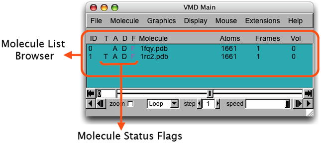
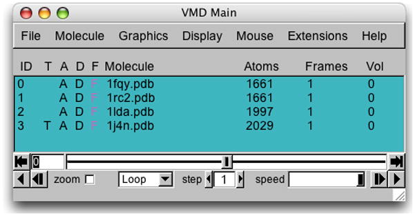
  You have just loaded two molecules. Any number of molecules can be loaded and displayed in VMD simultaneously by repeating the previous step. VMD can load as many molecules as the memory of your computer allows.

  Take a look at your VMD Main window, which should look like Figure 19. Within the VMD Main menu you can find the Molecule List Browser (circled in Figure 19), which shows the global status of the loaded molecules. The Molecule List Browser displays information about each molecule, including Molecule ID (ID), the four Molecule Status Flags (T, A, D, and F, which stand for Top, Active, Drawn, and Fixed), name of the molecule (Molecule), number of atoms in the molecule (Atoms), number of frames loaded in the molecule (Frames), and the volumetric data loaded (Vol). Let us first start with the Molecule column. By default the Molecule column displays file names of the molecules loaded in VMD, but you can change the molecule names to recognize them more easily.

Figure 19.

The Molecule List Browser.

Changing molecule names

• 4. In the VMD Main menu, double-click on 1fqy.pdb in the Molecule column. A window will pop up with the message “Enter a new name for molecule 0:”. Type in human aquaporin, and click OK (or press enter). In the VMD Main menu, the first molecule now has the name “human aquaporin”.

• 5. Repeat the previous step for the E. coli aquaporin by double-clicking the 1rc2.pdbmolecule name, and changing it to “E. coli aquaporin” in the pop-up window.

Drawing different representations for different molecules

Before we continue exploring other features in the Molecule List Browser, take a look at your OpenGL Display window. You have two aquaporin structures, but since they are both shown in the same default representation, it is difficult to distinguish them. To tell them apart, you can assign them different representations.

• 6. Open the Graphical Representations window via Graphics → Representations… from the VMD Main menu. Make sure “0:human aquaporin” is selected in the Selected Molecule pull-down menu on top. Select NewCartoon for Drawing Method, and ColorID → 1 red for Coloring Method.

• 7. In the Graphical Representations window, select “1:E. coli aquaporin” in the Selected Molecule pull-down menu on top. Select NewCartoon for Drawing Method, and ColorID → 4 yellow for Coloring Method. Close the Graphical Representations window.

  Now your OpenGL Display window should show a human aquaporin colored in red and an E. coli aquaporin colored in yellow.

Molecule Status Flags

In your OpenGL Display window, try moving the aquaporins around with your mouse in different mouse modes (rotating, scaling, and translating). You can see that both aquaporings move together. You can fix any molecule by double-clicking the F (fixed) flag in the Molecule List Browser on the left of the molecule name.

• 8. In the Molecule List Browser, double-click on the “F” flag on the left of “human aquaporin” to fix the human aquaporin molecule. Return to the OpenGL Display window and toggle your mouse around. You can see that only the yellow E. coli aquaporin moves. Double-click on the “F” flag for human aquaporin again to release it.

  One thing to notice about the F flag is that, although it may seem that one molecule has been moved relative to another when one of the molecules is fixed, the difference is only apparent. The internal coordinates of molecules are not changed by the rotation, translation and scaling motions. To change the coordinates of atoms in a molecule you need to use the text command interface (discussed in Basic Protocol ??), and by using the atom move picking modes (by choosing Mouse → Move in the VMD Main menu).

  Other features in the Molecule List Browser includes the Molecule ID (ID), Top (T), Active (A), and Drawn (D). Molecule ID is a number (starting from 0) assigned to each molecule when it is loaded into VMD, and permits VMD to recognize each molecule internally. You also refer to molecules by their Molecule IDs in the text command interface. Top flag (T) indicates the default molecule in VMD operations, for example when resetting the VMD OpenGL view and when playing molecule trajectories. There can be only one top molecule at a time. Active flag (A) indicates if the trajectory of the given molecule is updated when using animation tools described in Basic Protocol 2.

  Finally, Drawn flag (D) indicates if the given molecule is displayed in the OpenGL window. Let us try out the Top and Drawn flags.

• 9. Make sure no molecule is fixed. By default the last molecule loaded in the VMD is the top molecule, so you can check and see that there is a T displayed for the E. coli aquaporin in the VMD Main menu.

• 10. Reset the view by pressing the “=” key on the keyboard while keeping the OpenGL Display window active. Note that the yellow E. coli aquaporin is now placed in the center of the OpenGL Display window.

• 11. Switch the top molecule by double-clicking on the empty “T” flag for the human aquaporin molecule in the VMD Main menu. A “T” should appear for the human aquaporin, while the “T” for E. coli disappears. Go to the OpenGL Display window and reset the view again. You can see that this time the red human aquaporin is placed in the center of the OpenGL Display window.

• 12. In the VMD Main menu, try hiding a molecule by double-clicking on its “D” flag. You can display the molecule again by double-clicking its “D” flag again.

Basic Protocol 10

Aligning Molecules with the measure fit Command

When you look at your OpenGL Display window, you can see that the two aquaporins are very similar in structure. But it is difficult to detect their slight structural differences as the two proteins are placed apart. We will now try out a very useful Tcl command measure fit to align two molecules.

Open the VMD TkConsole window by choosing Extension → TkConsole from the VMD Main menu, and input the following commands:

set sel0 [atomselect 0 all]
set sel1 [atomselect 1 all]
set M [measure fit $sel0 $sel1]
$sel0 move $M
  measure fit 
selection1 selection2 – measures the transformation matrix that best aligns the coordinates of selection1 with the coordinates of selection2

As soon as you enter the last command line, you can see that the two aquaporins are now overlapping (Figure 20). The α-helical regions of the aquaporings agree very well, with bigger deviations in the loop regions. Note that the measure fit command can only work if two molecules have the same number of atoms. In this case it is a pure coincidence that the human aquaporin and E. coli aquaporin PDB files have the same number of atoms. The measure fit command is hence most useful in aligning the same protein in different conformations or different frames of a molecular dynamics simulation trajectory. Generally, to compare the structures of different proteins, one needs to use a different method. A good tool is the MultiSeq VMD plugin, which we will discuss in the following section.

Figure 20.

Result of the alignment between the two aquaporins using the measure fit command.

COMPARING PROTEIN STRUCTURES AND SEQUENCES WITH THE MULTISEQ PLUGIN

MultiSeq (Roberts et al., 2006) is a bioinformatics analysis environment developed in the Luthey-Schulten Group at the University of Illinois in Urbana-Champaign. MultiSeq allows users to organize, display, and analyze both sequence and structure data for proteins and nucleic acids, and has been incorporated in VMD as a plugin tool starting with VMD version 1.8.5 (MultiSeq homepage: http://www.scs.uiuc.edu/~schulten/multiseq). In this section you will learn how to compare protein structures and sequences with the VMD MultiSeq plugin. We will again use the water transporting channel protein, aquaporin, as an example.

Necessary Resources

Hardware

Computer

Software

VMD, and a text editor

Files

1fqy.pdb, 1rc2.pdb, 1lda.pdb, 1j4n.pdb and spinach_aqp.fasta, which can be downloaded

Basic Protocol 11

Structure Alignment with MultiSeq

Very often comparing structures of different proteins reveals important information. For example, proteins with similar functions tend to exhibit similar structural features. MultiSeq structure alignment is useful for this reason. We will compare the structures of four aquaporin proteins listed in Table 8.

Table 8.

The four aquaporins used in this section.

PDB code	Description	Reference
1fqy	Human AQP1	(Murata et al., 2000)
1rc2	E. coli AqpZ	(Savage et al., 2003)
1lda	E. coli Glycerol Facilitator (GlpF)	(Tajkhorshid et al., 2002)
1j4n	Bovine AQP1	(Sui et al., 2001)

Loading aquaporin structures

• 1. Start a new VMD session. Open the Molecule File Browser window by choosing the File → New Molecule… menu item in the VMD Main window. In the Molecule File Browser window, use the Browse… button to find and select the file 1fqy.pdb. Press Load to load the molecule.

• 2. Load the remaining aquaporins, 1rc2, 1lda, and 1j4n. Make sure that each pdb file is loaded into a new molecule. Close the Molecule File Browser window when you have loaded all four molecules. Your VMD Main menu should look like Figure 21 when all four aquaporins are loaded.

Figure 21.

VMD Main menu after loading the four aquaporins.

Aligning the molecules

• 3. Within the VMD main window, choose the Extension menu and select Analysis → MultiSeq.

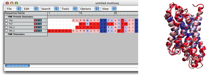
  The MultiSeq window (with window name untitled.multiseq showing at the top) should now be open. You may be asked to update some databases in a pop-up window if this is the first time you use MultiSeq. If this is the case, simply click “Yes” and wait for MultiSeq to finish downloading. When MultiSeq starts, your MultiSeq window should display a list of the four aquaporin protein structures and a list of two non-protein structures. The non-protein structures are detergent molecules used in crystallizing the aquaporin proteins, and will not be needed for structure or sequence alignment. You can tell MultiSeq to discard molecules you are not interested in.

• 4. In the MultiSeq window, select the 1lda_X detergent molecule by clicking on it. This will highlight the entire row of 1lda_X. Remove it from MultiSeq by pressing the delete or Backspace key on your keyboard. Do the same to remove the 1j4n_X detergent molecule.

  MultiSeq uses the program STAMP (Russel et al., 1992) to align protein molecules. STAMP (Structural Alignment of Multiple Proteins) is a tool for aligning protein sequences based on three-dimensional structures. Its algorithm minimizes the C_α distance between aligned residues of each molecule by applying globally optimal rigid-body rotations and translations. Note that you can only perform alignments on molecules that are structurally similar; if you try to align proteins that have no common structures, STAMP will fail.

• 5. In the MultiSeq window, select Tool → Stamp Structural Alignment. This will open the Stamp Alignment Options window.

• 6. In the Stamp Alignment Options window, choose “Align the following: All Structures” and go to the bottom of the menu and press “OK”.

  The molecules have been aligned. You can see the alignment both in the OpenGL window and in the MultiSeq window (Figure 22). Your alignment in OpenGL window will not immediately resemble Figure 22. When MultiSeq completes an alignment, it creates a new representation for all the aligned proteins in the NewCartoon representation with the same default coloring method and hides all other representations created previously. Let us give different colors to different aquaporins to distinguish them.

• 7. Open your Graphical Representations window, and you should see two representations for each molecule, the first one created when VMD loaded the molecule (which is now hidden), and the second one created automatically by MultiSeq. Select “0:1fqy.pdb” in the Selected Molecule pull-down menu on top and highlight the bottom representation by clicking on it. Change the color for this representation by selecting ColorID → 1 red for Coloring Method.

• 8. In the Graphical Representations window, select “1:1rc2.pdb” in the Selected Molecule pull-down menu on top and highlight the bottom representation by clicking on it. Select ColorID → 4 yellow for Coloring Method.

• 9. In the Graphical Representations window, select “2:1lda.pdb” in the Selected Molecule pull-down menu on top and highlight the bottom representation by clicking on it. Select ColorID → 11 purple for Coloring Method.

• 10. In the Graphical Representations window, select “3:1j4n.pdb” in the Selected Molecule pull-down menu on top and highlight the bottom representation by clicking on it. Select ColorID → 12 lime for Coloring Method. Close the Graphical Representations window.

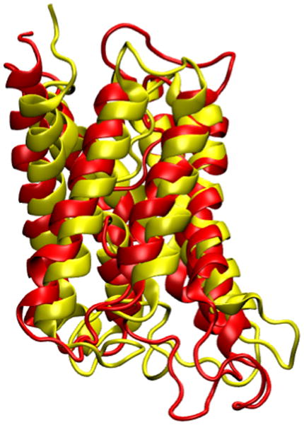
  Now your OpenGL window should look similar to Figure 22, and you can see that the alignment was pretty good as the four aquaporin structures are very similar.

Figure 22.

The four aquaporins aligned according to their structural similarity.

You can get more information about the alignment in the MultiSeq window by highlighting the molecules you wish to compare.

• 11. In the MultiSeq window, highlight 1fqy by clicking on it.

• 12. To highlight another molecule without unhighlighting 1fqy, you need to Ctrl-click (or command-click on a Mac) on that molecule. Highlight 1rc2 by clicking on it while holding down the Ctrl key on the keyboard (or the command key on a Mac).

  When both 1fqy and 1rc2 are highlighted, you should see at the lower left corner in the MultiSeq window a line of text: QH:0.6442, RMSD:2.3043, Percent Identity:30.28. Note that the values you obtain might be a little different depending on if your MultiSeq database is updated, but they should be close to the ones given here.

  The Q_H value is a metric for structural homology. It is an adaptation of the Q value that measures structural conservation (Eastwood et al., 2001). Q=1 implies that structures are identical. When Q has a low score (0.1–0.3), structures are not aligned well, i.e., only a small fraction of C_α atoms superimpose. Along with RMSD and Percent Identity, these numbers tell you that the 1fqy and 1rc2 structures are pretty well aligned. You can repeat the previous step to compare the alignment of other molecules. To unselect a highlighted molecule, Ctrl-click on it again (or command-click on a Mac).

Coloring molecules according to structural identity

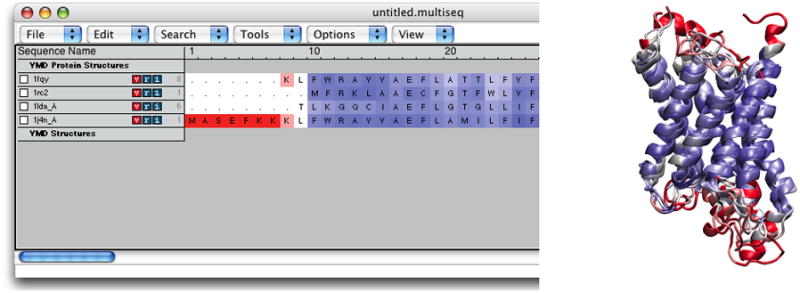
You can also color the molecules according to the value of Q per residue (Q_res) obtained in the alignment. Q_res is the contribution from each residue to the overall Q value of aligned structures.

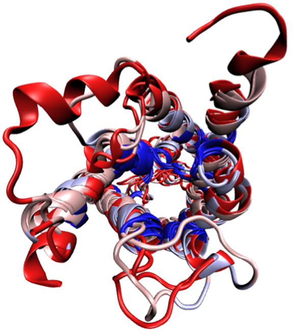
• 13. In the MultiSeq window, choose View → Coloring → Qres.

  Look at the OpenGL window to see the impact this selection has made on the coloring of the aligned molecules (Figure 23). Blue areas indicate that the molecules are structurally conserved at those points, red areas indicates that there is no correspondence in structure at those points. As you can see, the α-helices that form the pore are well conserved structurally among the four aquaporins, while there are more structural differences in the less functionally relevant loops.

Figure 23.

Result of a structural alignment of the four aquaporins, colored by Q_res.

Basic Protocol 12

Sequence Alignment with MultiSeq

Besides revealing structural similarities, MultiSeq also allows comparison of proteins based on their sequences. Sequence alignment is often used to identify conserved residues among similar proteins, as such residues are likely of functional importantance.

Aligning and coloring molecules by degree of conservation

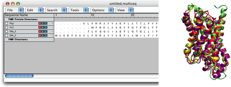
• 1. In the MultiSeq window, select Tools → ClustalW Sequence Alignment.

• 2. In the ClustalW Alignment Options window, make sure the “Align All Sequences” option is checked, and go to the bottom of the window and select “OK”. Now the four aquaporins have been aligned according to their sequence using the ClustalW tool (Thompson et al., 1994).

• 3. Let us color the aligned molecules by their sequence similarity. In the MultiSeq window, choose View→ Coloring → Sequence identity.

  Now each amino acid is colored according to the degree of conservation within the alignment: blue means highly conserved, red means low or no conservation. Your MultiSeq window and OpenGL window should resemble Figure 24.

  You have now aligned the four aquaporins according to their sequence and identified the conserved residues, found mainly inside the pore (Figure 25). Since aquaporin facilitates water transport cross the membrane, these conserved residues are most likely the ones that carry out this function.

Figure 24.

Result of a sequence alignment of the four aquaporins, colored by sequence identity.

Figure 25.

Top view of the aligned aquaporins colored by sequence conservation. The conserved residues locate mostly inside the aquaporin pore.

Importing FASTA files for sequence alignment

Many times the structure of a protein might not be available, but its sequence is. You can analyze a protein in MultiSeq without its structure by loading its sequence information in the FASTA file format. If you do not have the FASTA file of a protein but you have its sequence, you can create a FASTA file easily with any text editor of your choice.

• 4. Find the provided FASTA sequence file spinach_aqp.fasta and open it with a text editor.

  A FASTA file contains a header that starts with “>”, followed by the name of the protein. In the next line is the protein sequence in one-letter amino acid code. You can create FASTA files similarly in this format. When you create a FASTA file, remember to save it in plain text, and use .fasta as the file extension.

• 5. Close the text editor when you finish examining spinach_aqp.fasta.

• 6. In the MultiSeq window, select File → Import Data…. Select “From File” in the Import Data window, and press the top Browse button on top to select the file spinach_aqp.fasta. Press OK on the bottom of the Import Data window.

  You have now loaded the sequence of a spinach aquaporin into MultiSeq. You can now perform sequence alignment on the spinach aquaporin protein with other loaded aquaporin molecules. Let us try a sequence alignment between a spinach and a human aquaporin.

• 7. Click on the checkbox on the left of spinach_aqp, and click on the checkbox on the left of 1fqy.pdb.

• 8. Open the ClustalW Alignment Options window by selecting Tools → ClustalW Sequence Alignment. Under the Multiple Alignment options on the top, check Align Marked Sequences. Go to the bottom of the window and select OK.

  The sequence of spinach aquaporin is now aligned with the sequence of human aquaporin, and you can check how good the alignment is by obtaining its Q_H and Sequence Identity values. If you feel that the two molecules are listed too far apart in the MultiSeq window, you can move the molecules by dragging them with your mouse. Also, as you might have noticed, in MultiSeq molecules can be “Marked” by checking their checkboxes. They can also be “Selected” by highlighting them. You can align only the molecules of your choice by selecting Align Marked Sequences or Align Selected Sequences, depending if you have marked or highlighted your molecules. This option is available for both structural alignment and sequence alignment.

  The structure of spinach aquaporin is actually available (Tornroth-Horsefield et al., 2006), but now that you have learned how to import FASTA sequence data, you can compare the sequences of proteins even if their structures are not resolved yet experimentally.

• 9. When you finish comparing the sequence of spinach aquaporin with other aquaporins, delete it by clicking on spinach_aqp and press delete or Backspace on your keyboard.

Basic Protocol 13

Creating a Phylogenetic Tree with MultiSeq

The Phylogenetic Tree feature in MultiSeq elucidates the structure-based and/or sequence-based relationships between different proteins. Structure-based phylogenetic trees can be constructed according to the RMSD or Q values between the molecules after alignment; sequence-based phylogenetic trees can be constructed according to the percent identity or ClustalW values (Thompson et al., 1994).

• 1. Align the structures again by going to the Multiseq window and selecting Tools→Stamp Structural Alignment.

• 2. In the Stamp Structural Alignment window, select All Structures, and keep the default values for the rest of the parameters. Press the OK button to align the structures.

• 3. In the Multiseq program window choose Tools → Phylogenetic Tree. The Phylogenetic tree window will open.

• 4. Select Structural tree using Q_H, and press the OK button.

  A phylogenetic tree based on the Q_H values should be calculated and drawn as shown in Figure 25. Here you can see the relationship between the four aquaporins, e.g., how the E. coli AqpZ (1r2c) is related to human AQP1 (1fqy).

• 5. You can also construct the phylogenetic tree of the four aquaporins based on their sequence information. Close the Tree Viewer window.

• 6. You need to perform the sequence alignment again for the four aqauporin proteins. In your MultiSeq window, choose Tools → ClustalW Sequence Alignment, and make sure the “Align All Sequences” option is checked, and press OK.

• 7. In the Multiseq program window choose Tools → Phylogenetic Tree to open the Phylogenetic tree window again.

• 8. Select “Sequence tree using ClustalW”, and press the “OK” button. A phylogenetic tree based on ClustalW will be calculated and drawn as shown in Figure 26.

• 9. Quit VMD.

Figure 26.

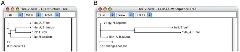
(A) A structure-based phylogenetic tree generated by Q_H values. (B) A sequence-based phylogenetic tree generated by ClustalW.

DATA ANALYSIS IN VMD

VMD is a powerful tool for analysis of structures and trajectories. Numerous tools for analysis are available under the VMD Main menu item Extension → Analysis. In addition to these built-in tools, VMD users often use custom-written scripts to analyze desired properties of the simulated systems. VMD Tcl scripting capabilities are very extensive, and provide boundless opportunities for analysis. In this section, we will learn how to use built-in VMD features for standard analysis, as well as consider a simple example of scripting.

Necessary Resources

Hardware

Computer

Software

VMD, a text editor, and a plotting application

Files

ubiquitin.psf, pulling.dcd, equilibration.dcd and distance.tcl, which can be downloaded

Basic Protocol 14

Adding Labels in VMD

Labels can be placed in VMD to get information on a particular selection, to be used during visualization and quantitative analysis. Labels are selected with the mouse and can be accessed in Graphics → Labels menu. We will cover labels that can be placed on atoms and bonds, although angle and dihedral labelings are also available. In this context, labels for “bonds” or “angles” actually mean distances between two atoms or angles between three atoms; the atoms do not have to be physically connected by bonds in the molecule.

• 1. Start a new VMD session. Load the ubiquitin trajectory into VMD (using the files ubiquitin.psf and pulling.dcd). For graphical representation, display protein only, using NewCartoon for drawing method and Structure for coloring method. If you need help, check Basic Protocol 3, steps 1–5.

• 2. Choose the Mouse → Labels → Atoms menu item from the VMD Main menu. The mouse is now set to the mode for displaying atom labels. You can click on any atom on your molecule and a label will be placed for this atom. Clicking again on it will erase the label.

• 3. We will now try the same for bonds. Choose the Mouse → Label → Bonds menu item from the VMD Main menu. This selects the “Display Label for Bond” mode.

  We will consider the distance between the α carbon of Lysine 48 and of the C terminus. In the pulling simulation, the former is kept fixed, and the latter is pulled at a constant force of 500 pN. In reality, polyubiquitin chains can be linked by a connection between the C terminus of one ubiquitin molecule and the Lysine 48 of the next. The simulation then mimics the effect of pulling on the C terminus with this kind of linkage.

• 4. Open the TkConsole window by selecting Extensions → Tk Console in the VMD Main menu. We will make a VDW representation for the α carbons of Lysine 48 and of the C terminus. To find out the indices of these atoms, make a selection including these two atoms by typing in the TkConsole window:

  sel [atomselect top “resid 48 76 and name CA”]
  

• 5. Get the indices by typing the following line in the TkConsole window:

  $sel get index
  

  This command should give the indices 770 1242.

  Note that the atom number of these atoms in the pdb file is 771 and 1243. This is because VMD starts counting atom indices from zero. This is only the case for index, since VMD does not read them from the PDB file. Other keywords, such as residue, are consistent with the PDB file.

• 6. In the Graphical Representations window, create a representation for the selection index 770 1242, with VDW as drawing method.

• 7. Now that you can see the two α-carbons, choose the Mouse → Label → Bonds menu item from the VMD Main menu. Click on each atom one after the other.

  You should get a line connecting the two atoms (Figure 27). The number appearing next to the line is the distance between the two atoms in Ångstroms. The value of the distance displayed corresponds to the current frame. Try playing the trajectory - you will see that the label is modified automatically as the distance between the atoms changes. Note that the appearance of the line (its color), as well as the appearance of essentially all other objects in VMD, can be changed in Graphics → Colors in the VMD Main menu.

  The shortcut keys for labels are 1: Atoms and 2: Bonds. You can use these instead of the Mouse menu. Be sure the Open GL Display window is active when using these shortcuts.

• 8. The labels can be used not only for displaying, but also for obtaining quantitative information. In VMD Main menu, select Graphics → Labels. On the top left-hand side of the window, there is a pull-down menu where you can choose the type of label (Atoms, Bonds, Angles, Dihedrals). For now, keep it in Atoms. You can see the list of atoms for which you have made a label.

• 9. Click on one of the atoms. You can see all the information of the atom displayed on the bottom half of the Labels window. This information is useful to make selections; it corresponds to the current frame, and is updated as the frame is changed.

• 10. You can also delete, hide, or show the atom label by clicking on the corresponding button on the top of the Labels window.

• 11. In the Labels window, choose label type Bonds, and select the “bond” (distance) you labeled (Figure 27). The information given corresponds to only the first atom in the bond, but the number in the “Value” field corresponds to the length of the bond in Ångstroms.

• 12. Click on the “Graph” tab. Select the bond you labeled between atoms 770 and 1242. Click on the Graph button. This will create a plot of the distance between these two atoms over time (Figure 27). You can also save this data to a file by clicking on the “Save” button, and then use an external plotting program to visualize the data.

• 13. Quit VMD.

Figure 27.

Labels in VMD.

Basic Protocol 15

Example of a built-in analysis tool: the RMSD Trajectory Tool

The built-in analysis tools in VMD are available under the menu item Extension → Analysis. These tools each features a GUI window that allows one to enter parameters and customize the quantities analyzed. In addition, all tools can be invoked in a scripting mode, using the TkConsole window. We will learn how to work with one of the most frequently used tools, the RMSD Trajectory Tool.

In this example, we will analyze RMSD for two trajectories for the same system, ubiquitin.psf. One of them is the already familiar pulling trajectory, pulling.dcd, and the other is the trajectory of a simulation in which no force was applied to the protein, equilibration.dcd.

• 1. Start a new VMD session. Load the ubiquitin equilibration trajectory into VMD (using the files ubiquitin.psf and equilibration.dcd).

• 2. Choose Extension → Analysis → RMSD Trajectory Tool in the VMD Main window (Figure 28). The RMSD Trajectory Tool window will show up.

  In the RMSD Trajectory Tool window you can see many customization options. For the default values, the molecule to be analyzed is ubiquitin.psf (the only one loaded). The selection for which RMSD will be computed is all of the protein atoms, excluding hydrogens (since the “noh” checkbox is on). The RMSD will be calculated for each frame with the reference to frame 0. Make sure the “Plot” checkbox is selected.

• 3. Click the “Align” button.

  This will align each frame of the trajectory with respect to the reference frame (in this case, frame 0) to minimize the RMSD, by applying only rigid-body translations and rotations. This step is not necessary, but is desirable in most cases, because we are interested only in RMSD that arises from the fluctuations of the structure and not from the displacements and rotations of the molecule as a whole. The result of the alignment can be seen in the OpenGL display.

• 4. Click the “RMSD” button in the RMSD Trajectory Tool window. The protein RMSD (in Ångstrom) vs. frame number is displayed in a plot (Figure 28).

  Over several initial frames, RMSD=0 because positions of the protein atoms are fixed during that time in the simulation to allow water molecules around the protein to adjust to the protein surface. After that, the protein is released, and the RMSD grows quickly to around 1.5Å. At that point, the RMSD levels off and remains at ~1.5Å further on. This is a typical behavior for molecular dynamics simulations. Leveling of the RMSD means that the protein has relaxed from its initial crystal structure (which is affected by crystal packing and usually misses some atoms, e.g., hydrogens) to a more stable one. Production molecular dynamics simulations are usually preceded by such equilibration runs, where the protein is allowed to relax; the process is monitored by checking RMSD vs. time, and equilibration is assumed to be sufficient when RMSD levels off. The RMSD of 1.5Å is an acceptable value for most protein simulations. Usually, the deviations from the crystal structure in a simulation are due to the thermal motion and to the relaxation process mentioned; imperfections of the simulation force-fields contribute as well.

• 5. We will now work with the other trajectory, in which the ubiquitin is pulled apart. Load this trajectory into VMD using the files ubiquitin.psf and pulling.dcd. Make sure you load ubiquitin.psf as a new molecule. You can change the names of the molecules by double-clicking on them in the VMD Main menu (see Basic Protocol 9, steps 4 and 5).

• 6. In the RMSD Trajectory Tool window, hit the button “Add all” to update the list of molecules.

• 7. Click the “Align” button, and then click “RMSD”.

  The new graph (Figure 29) displays two RMSD plots vs. time, one for the equilibration trajectory, and the other for the pulling trajectory. The RMSD for the pulling trajectory does not level off and is much higher than those in the equilibration trajectory, since the protein is stretched in the simulation.

• 8. Quit VMD.

Figure 28.

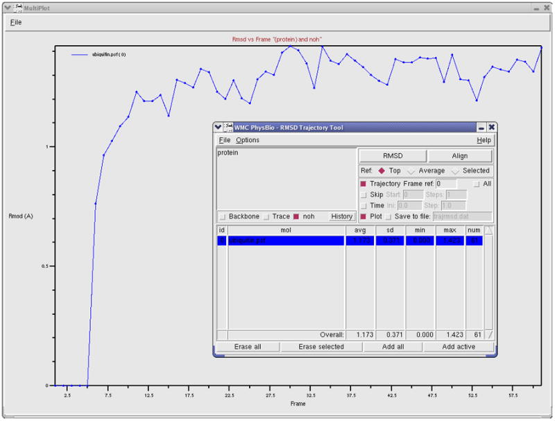
RMSD Trajectory Tool. The RMSD is plotted for the equilibration of ubiquitin.

Figure 29.

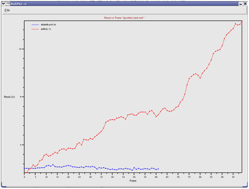
RMSD vs. time for the equilibration (blue) and pulling (red) trajectories of ubiquitin.

Basic Protocol 16

Example of an Analysis Script

In many cases, one requires special types of trajectory analysis that are tailored for certain needs. The Tcl scripting in VMD provides opportunities for such custom tasks. Users commonly write their own scripts to analyze the features of interest. A very extensive library of VMD scripts, contributed by many users, is available online (http://www.ks.uiuc.edu/Research/vmd/script_library/). Here we will explore a very simple exemplary script, distance.tcl, which computes the distance between two atom selections vs. time and the distribution of the distances.

• 1. Start a new VMD session. Load the ubiquitin equilibration trajectory (files ubiquitin.psf and equilibration.dcd).

• 2. Open the TkConsole window by selecting Extension→ Tk Console in the VMD Main menu.

• 3. In the the TkConsole window, load the script into VMD by typing: source distance.tcl (make sure that the file distance.tcl is in the current folder). This will load the procedure defined in distance.tcl into VMD.

• 4. One can now invoke the procedure by typing distance in the TkConsole window. In fact, the correct usage is

  distance seltext1 seltext2 N_d f_r_out f_d_out
  

  where seltext1 and seltext2 are the selection texts for the groups of atoms between which the distance is measured, N_d is the number of bins for the distribution, and f_r_out and f_d_out are the file names to where the output distance vs. time and distance distribution will be written.

• 5. Open the script file distance.tcl with a text editor. You can see that the script does the following:

  1. Choose atom selections:

     set sel1 [atomselect top “$seltext1”]
     set sel2 [atomselect top “$seltext2”]
     

  2. Get the number of frames in the trajectory and assign this value to the variable nf:

     set nf [molinfo top get numframes]
     

  3. Open file specified by the variable f_r_out:

     set outfile [open $f_r_out w]
     

  4. Loop over all frames

     {set i 0} {$i < $nf} {incr i} {
     

  5. Write out the frame number and update the selections to the current frame:

     puts “frame $i of $nf”
     $sel1 frame $i
     $sel2 frame $i
     

  6. Find the center of mass for each selection (com1 and com2 are position vectors):

     set com1 [measure center $sel1 weight mass]
     set com2 [measure center $sel2 weight mass]
     

  7. At each frame i, find the distance by subtracting one vector from the other (command vecsub) and computing the length of the resulting vector (command veclegth), assign that value to an array element simdata($i.r), and print a frame-distance entry to a file:

     set simdata($i.r) [veclength [vecsub $com1 $com2]]
     puts $outfile “$i $simdata($i.r)”
     }
     

  8. Close the file

     close $outfile
     

  9. The second part of the script is for obtaining the distance distribution. It starts from finding the maximum and minimum values of the distance.

     set r_min $simdata(0.r)
     set r_max $simdata(0.r)
     for {set i 0} {$i < $nf} {incr i} {
     set r_tmp $simdata($i.r)
     if {$r_tmp < $r_min} {set r_min $r_tmp}
     if {$r_tmp > $r_max} {set r_max $r_tmp}
     }
     

  10. The step over the range of distances is chosen based on the number of bins N_d defined in the beginning, and all values for the elements of the distribution array are set to zero.

      set dr [expr ($r_max - $r_min)/($N_d - 1)]
      for {set k 0} {$k < $N_d} {incr k} {
      set distribution($k) 0
      }
      

  11. The distribution is obtained by adding 1 (incr…) to an array element every time the distance is within the respective bin:

      for {set i 0} {$i < $nf} {incr i} {
      set k [expr int(($simdata($i.r) - $r_min)/$dr)]
      incr distribution($k)
      }
      

  12. Write out the file with the distribution:

      set outfile [open $f_d_out w]
      for {set k 0} {$k < $N_d} {incr k} {
      puts $outfile “[expr $r_min + $k $dr] $distribution($k)”
      }
      close $outfile
      

• 6. Now run the script by typing in the TkConsole window:

  distance “protein” “protein and resid 76” 10 res76-r.dat\ res76-d.dat
  

  This will compute the distance between the center of the protein and center of the terminal residue 76, and write the distance vs. time and its distribution to files res76-r.dat and res76-d.dat.

• 7. Repeat the same for the protein’s residue 10 by typing in the TkConsole window:

  distance “protein” “protein and resid 10” 10 res10-r.dat\ res10-d.dat
  

  The data in files produced by the script distance.tcl are in two-column format. Compare the outputs for residue 76 and 10 using your favorite external plotting program (Figure 30).

  Residue 76 is at the protein’s C-terminus, which is extended towards the solvent and is quite flexible, while residue 10 is at the surface of the globular part of ubiquitin. The difference in their dynamics with respect to the rest of the protein is immediately obvious when our newly obtained data are plotted (Figure 30): the distance of residue 76 from the protein’s center is substantially greater than that of residue 10, and the distribution of the distance is noticeably wider due to the flexibility of the C-terminus. This is just a simple example of scripting for the analysis of a trajectory. Similar, but usually much more complex, customized scripts are routinely employed by VMD users to perform many kinds of analysis.

• 8. Quit VMD.

Figure 30.

Distance between a residue and the center of ubiquitin. The distances analyzed are those for residue 76 (black) and residue 10 (green).

COMMENTARY

Background Information

VMD has been developed by the Theoretical and Computational Biophysics Group at the University of Illinois at Urbana-Champaign. Throughout its developement, many features have been added, and user-specific functions can be implemented through embedded scripting languages like Python and Tcl, providing a wide spectrum of tools for the scientific community. Specifically, VMD is most suitable for high-resolution visualization and image rendering, preparation of molecular dynamics simulation systems and analysis of simulation results, and animation of molecular dynamics trajectory. In addition, VMD can also work with volumetric data, and provides a platform for bioinformatic analysis such as protein sequence alignment. What we are able to present in this tutorial only showcases a small part of VMD’s capability. But now that you have learned the basics of VMD, you are ready to explore its many other features most suitable for your research. For this purpose there are many tutorials available that aim at offering a more focused training, either on a specific tool or on a scientific topic. You can find many useful documentations, including the comprehensive VMD User’s Guide, in the VMD homepage http://www.ks.uiuc.edu/Research/vmd/.

Critical Parameters and Troubleshooting

Most parameters in VMD can be easily adjusted to suit individual users’ needs. For example, when rendering molecules using a representation, as described in Basic Protocal 1, users can adjust the resolution of the representation in the graphical user interface, as well as many other parameters specific to the drawing method of the representation. New users of VMD might find default settings for most parameters are good starting points, but are also encouraged to change the parameters and test the difference. If you have any questions on using VMD, we encourage you to subscribe to the VMD mailing list http://www.ks.uiuc.edu/Research/vmd/mailing_list/.

Figure 1.

Example renderings made with VMD (Freddolino et al., 2006; Yin et al., 2006; Yu et al., 2006; Sotomayor et al., 2007; Wang et al., 2007).

Figure 14.

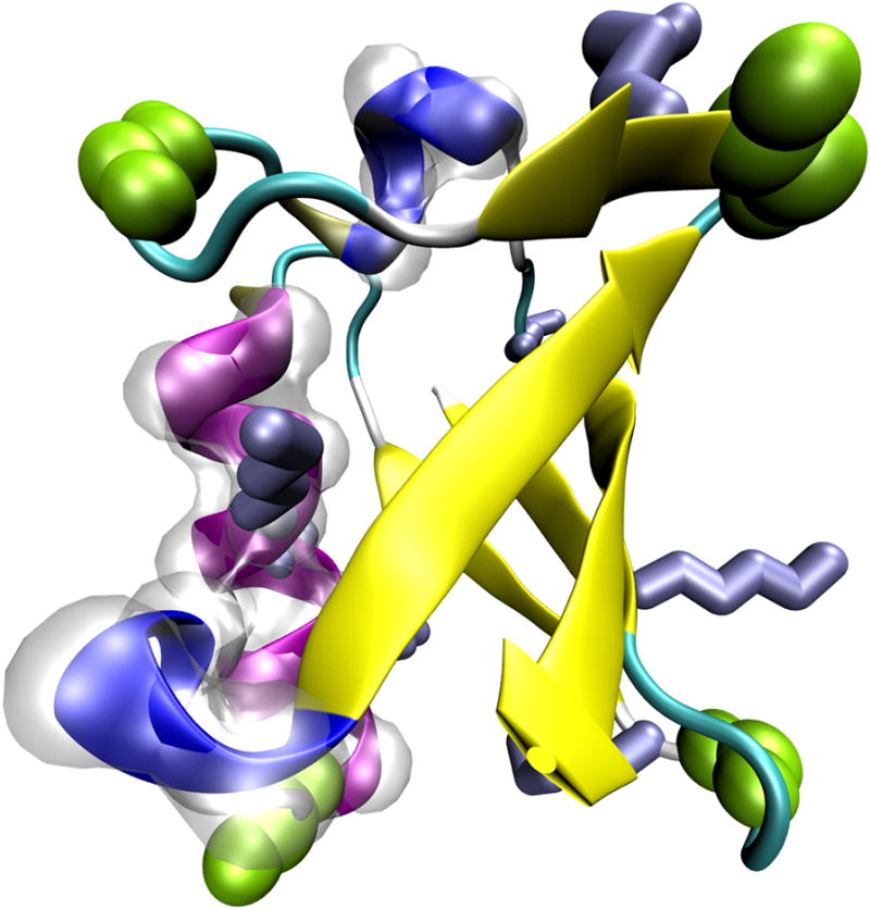
Example of a POV3 rendering.

Literature Cited

- Eastwood MP, Hardin C, Luthey-Schulten Z, Wolynes PG. Evaluating the protein structure-prediction schemes using energy landscape theory. IBM J Res Dev. 2001;45:475–497. [Google Scholar]
- Freddolino PL, Arkhipov AS, Larson SB, McPherson A, Schulten K. Molecular dynamics simulations of the complete satellite tobacco mosaic virus. Structure. 2006;14:437–449. doi: 10.1016/j.str.2005.11.014. [DOI] [PubMed] [Google Scholar]
- Frishman D, Argos P. Knowledge-based secondary structure assignment. Proteins. 1995;23:566–579. doi: 10.1002/prot.340230412. [DOI] [PubMed] [Google Scholar]
- Humphrey W, Dalke A, Schulten K. VMD – Visual Molecular Dynamics. J Mol Graphics. 1996;14:33–38. doi: 10.1016/0263-7855(96)00018-5. [DOI] [PubMed] [Google Scholar]
- Isralewitz B, Gao M, Schulten K. Steered molecular dynamics and mechanical functions of proteins. Curr Opin Struct Biol. 2001;11:224–230. doi: 10.1016/s0959-440x(00)00194-9. [DOI] [PubMed] [Google Scholar]
- Murata K, Mitsuoka K, Hirai T, Walz T, Agre P, Heymann JB, Engel A, Fujiyoshi Y. Structural determinants of water permeation through aquaporin-1. Nature. 2000;407:599–605. doi: 10.1038/35036519. [DOI] [PubMed] [Google Scholar]
- Phillips JC, Braun R, Wang W, Gumbart J, Tajkhorshid E, Villa E, Chipot C, Skeel RD, Kale L, Schulten K. Scalable molecular dynamics with NAMD. J Comp Chem. 2005;26:1781–1802. doi: 10.1002/jcc.20289. [DOI] [PMC free article] [PubMed] [Google Scholar]
- Roberts E, Eargle J, Wright D, Luthey-Schulten Z. MultiSeq: Unifying sequence and structure data for evolutionary analysis. BMC Bioinformatics. 2006;7:382. doi: 10.1186/1471-2105-7-382. [DOI] [PMC free article] [PubMed] [Google Scholar]
- Russel RB, Barton G. Multiple protein sequence alignment from tertiary struture comparison: assignment of global and resiude confidence levels. Proteins: Struct, Func, Gen. 1992;14:309–323. doi: 10.1002/prot.340140216. [DOI] [PubMed] [Google Scholar]
- Savage DF, Egea PF, Robles-Colmenares Y, O’Connell JD, III, Stroud RM. Architecture and selectivity in aquaporins: 2.5 Å X-ray structure of aquaporin Z. PLoS Biology. 2003;1:E72. doi: 10.1371/journal.pbio.0000072. [DOI] [PMC free article] [PubMed] [Google Scholar]
- Sotomayor M, Vasquez V, Perozo E, Schulten K. Ion conduction through MscS as determined by electrophysiology and simulation. Biophys J. 2007;92:886–902. doi: 10.1529/biophysj.106.095232. [DOI] [PMC free article] [PubMed] [Google Scholar]
- Sui H, Han BG, Lee JK, Walian P, Jap BK. Structural basis of water-specific transport through the AQP1 water channel. Nature. 2001;414:872–878. doi: 10.1038/414872a. [DOI] [PubMed] [Google Scholar]
- Tajkhorshid E, Nollert P, Jensen MØ, Miercke LJW, O’Connell J, Stroud RM, Schulten K. Control of the selectivity of the aquaporin water channel family by global orientational tuning. Science. 2002;296:525–530. doi: 10.1126/science.1067778. [DOI] [PubMed] [Google Scholar]
- Thompson JD, Higgins DG, Gibson TJ. CLUSTAL W: improving the sensitivity of progressive multiple sequence alignment through sequence weighting, position-specific gap penalties and weight matrix choice. Nucl Acids Res. 1994;22:4673–4680. doi: 10.1093/nar/22.22.4673. [DOI] [PMC free article] [PubMed] [Google Scholar]
- Törnroth-Horsefield S, Wang Y, Hedfalk K, Johanson U, Karlsson M, Tajkhorshid E, Neutze R, Kjellbom P. Structural mechanism of plant aquaporin gating. Nature. 2006;439:688–694. doi: 10.1038/nature04316. [DOI] [PubMed] [Google Scholar]
- Vijay-Kumar S, Bugg CE, Cook WJ. Structure of ubiquitin at 1.8Å resolution. JMB. 1987;194:531–544. doi: 10.1016/0022-2836(87)90679-6. [DOI] [PubMed] [Google Scholar]
- Wang Y, Cohen J, Boron WF, Schulten K, Tajkhorshid E. Exploring gas permeability of cellular membranes and membrane channels with molecular dynamics. J Struct Biol. 2007;157:534–544. doi: 10.1016/j.jsb.2006.11.008. [DOI] [PubMed] [Google Scholar]
- Yin Y, Jensen MØ, Tajkhorshid E, Schulten K. Sugar binding and protein conformational changes in lactose permease. Biophys J. 2006;91:3972–3985. doi: 10.1529/biophysj.106.085993. [DOI] [PMC free article] [PubMed] [Google Scholar]
- Yu J, Yool AJ, Schulten K, Tajkhorshid E. Mechanism of gating and ion conductivity of a possible tetrameric pore in Aquaporin-1. Structure. 2006;14:1411–1423. doi: 10.1016/j.str.2006.07.006. [DOI] [PubMed] [Google Scholar]