Political economy of marine reserves: Understanding the role of opportunity costs

Abstract

The creation of marine reserves is often controversial. For decisionmakers, trying to find compromises, an understanding of the timing, magnitude, and incidence of the costs of a reserve is critical. Understanding the costs, in turn, requires consideration of not just the direct financial costs but also the opportunity costs associated with reserves. We use a discrete choice model of commercial fishermen’s behavior to examine both the short-run and long-run opportunity costs of marine reserves. Our results can help policymakers recognize the factors influencing commercial fishermen’s responses to reserve proposals. More generally, we highlight the potential drivers behind the political economy of marine reserves.

Many scientists and marine conservationists are calling for increases in the number of no-take marine reserves throughout the world’s oceans (1, 2). As proposals to form new reserves move forward, commercial and recreational fishermen fear the short- and long-term effects on their livelihoods from lost access to particular fishing grounds. For example, proposals to site reserves near California’s Channel Islands and the Tortugas in Florida generated passionate political advocacy (3). More recently, controversy surrounding the California Marine Life Protection Act has intensified as fishermen and other stakeholders question the potential benefits and science behind proposed actions (4).

Advocates for marine reserves often treat fishermen’s assertions about the costs with the same skepticism that fishermen have for the stated benefits. For decisionmakers trying to find compromises between these and other stakeholders, an understanding of the costs and benefits of reserves is critical. This information is particularly relevant when reserve policies are determined through public stakeholder meetings that may be dominated by extreme rather than moderate representatives of all sides in the debate, including different parts of the fishing industry (5).

When a fisherman goes fishing, he purchases fuel, bait, etc., and he also forfeits opportunities to earn income in other activities, e.g., fishing elsewhere or working on land. Understanding the responses of commercial fishermen to marine reserves requires consideration of these opportunity costs. We use an empirically established model of a commercial fishery to predict fishermen’s opportunity costs both in the short and in the long run. Although many of our general findings appear in the natural resource economics literature (6–10), we highlight how these responses are driven by the way a reserve changes opportunities for fishermen: opportunities that arise in space (e.g., reserves eliminate some possible fishing grounds), in the biological domain (e.g., reserves affect the abundance of target species), and in the financial realm (e.g., reserves may alter the costs of fishing). We extend the literature by considering how these opportunities vary across fishermen with heterogeneous skills. Accounting for heterogeneity is a critical and often overlooked dimension in the literature on marine reserve implementation; those with the most to lose or gain tend to dominate public stakeholder meetings (5).

Our analysis allows us to sharpen the discussion on the intertemporal tradeoffs and tensions in the debate surrounding reserves (11). For example, proponents of reserves often focus on potential long-run benefits, which include the recovery of fish populations within (12) and “spillovers” outside the reserve (13, 14). Opponents, on the other hand, focus on potential short-run costs, primarily the loss of fishing opportunities (3). Describing the time profile of costs enables us to isolate the factors that determine whether fishermen’s opportunity costs rise or fall with time.

We postulate that if the current opportunity costs of fishing are high (i.e., if there are good opportunities elsewhere) and if fishermen perceive longer term benefits such as stock enhancement outside the reserve, they are less likely to oppose reserve creation (15). Identification of the factors determining these costs and benefits can improve a policymaker’s ability to navigate the debate and inform the choice of where—what fishery and what area within the fishing grounds—to site a marine reserve.

Results

To gain insights into the political economy of marine reserves, we present results for the short run and long run that are derived from a model that has been used extensively in empirical economic research to quantify the drivers of fishing behavior across a wide range of commercial fisheries (16–23) (SI Appendix A1, Fig. S1). We define the short run as the period immediately after a reserve is created, during which fishermen, but not fish, are able to respond to the new circumstances. Based on the recovery times of the relevant population(s), this time span might be three to five years or more, depending on the species (12). In the long run, fishermen make repeated decisions about where to fish because the profitability of each site changes over time as fish population levels adjust. In both settings, we first assume that all fishermen have the same skill; then we investigate the implications of heterogeneity in fishing skill.

Without loss of generality, we assume that forming a reserve eliminates the Jth location from the set of fishable sites. Given the assumptions of the short-run model (see Methods), we derive a closed-form expression for a fisherman’s expected willingness to pay (WTP) to avoid forming a reserve. WTP is a standard metric in economics that represents the (often hypothetical) financial compensation that would be necessary to make a person as well off after a policy change as before the change. It may be positive (“What would you, personally, be willing to pay to preserve a grove of old-growth trees?”) or negative (“What would you, personally, want to be paid in compensation for the loss of this grove?). WTP, consequently, is the difference between the income earned by fishing in the area of the proposed reserve and the fisherman’s next best alternative, in the rest of the fishery or ashore, and is an indicator of likely opposition. We vary the parameters of the model to understand the circumstances in which creating a marine reserve is likely to generate more or less opposition. The short-run results, assuming homogeneous fishermen, are presented in SI Appendix A2.

Result one (r.1 in Table 1) states that opposition to reserves is likely to be less when nonfishery earning opportunities are high (compared with an otherwise similar fishery). A favorable nonfishery option could reflect an abundance of jobs outside the fishery, high wages in these jobs, lucrative opportunities to fish for other species, or a high value of leisure. We use nonfishery “wages” or “earnings” as heuristics to refer to any of these conditions. In fisheries where nonfuel costs of fishing (e.g., bait and ice) are high (r.2), fishermen sacrifice less when a reserve is created and are less likely to oppose a reserve. Because the abundance of fish can vary across reserve and nonreserve sites, fish prices and fuel costs can lead to either more or less opposition to reserves (r.3 and r.4). In essence, when fish prices are high, the value of the reserve site is higher, but the value of all other sites is also higher and the relative value of the nonfishing alternative is lower.

Table 1.

An increase in each characteristic increases, decreases, or has an ambiguous effect on opposition to forming a marine reserve

Result	Biological or economic characteristic	Opposition
All sites
1	Nonfishery opportunity cost	Decreases
2	Nonfuel cost of making a fishing trip (bait, ice, etc.)	Decreases
3	Ex-vessel price per pound of fish	Ambiguous
4	Price per gallon of fuel	Ambiguous
Nonreserve sites
5	Level of the fish stock at any of the remaining fishing sites	Decreases
6	Efficiency of a unit of fishing effort at any of the remaining fishing sites	Decreases
7	Distance from port to a nonreserve site	Increases
Reserve site
8	Level of the fish stock at the reserve site before closure	Increases
9	Efficiency of a unit of fishing effort at the reserve site before closure	Increases
10	Distance from port to the reserve site	Decreases

Ambiguous captures cases where we are unable to sign the effect without imposing additional assumptions on the characteristics of the system.

Support for a reserve is likely to be greater the larger the stock in the nonreserve sites (r. 5) because catching a lot of fish in one of the remaining fishing grounds is similar to having a lucrative alternative job. The intuition is the same for travel distance and catchability in the remaining fishing sites (r. 6 and 7). Generally, the more important the nonreserve sites are to the profitability of commercial fishermen, the weaker the opposition to the reserve. And the more profitable the fishing in the reserve site before its closing, the stronger the opposition (r. 8–10).

The results in Table 1 are based on a representative fisherman, but fishermen do not all respond to profit opportunities in the same way (19, 24). We explore the effect of different fishing skills among fishermen in Fig. 1; a policy that leads to a modest short-run cost for most fishermen may lead to a large short-run cost for a low-skilled or high-skilled fisherman. Fig. 1 Upper illustrates that opposition to a reserve hinges critically on the level of the fish stocks inside and outside the reserve before its closing. The general pattern is consistent with Table 1, in that higher stocks outside the reserve reduce opposition, and a higher stock at the reserve site increases opposition. However, in a fleet characterized by heterogeneous skill, opposition is not uniform. When prereserve stocks are less (more) abundant outside the reserve than inside, high-skill fishermen will tend to oppose reserves more (less) than low-skill fishermen. Only when prereserve stocks inside and outside are the same do low- and high- skill fishermen have comparable levels of opposition (where the lines in Fig. 1 Upper). This finding suggests that when fishing returns are spatially uniform, stakeholder meetings are likely to attract average fishermen, but in a fishery with large variations in the spatial distribution of fish abundance and returns to fishing, meetings are likely to attract fishermen from one extreme or the other of the skill distribution (5).

Fig. 1.

Variation in opposition to reserves from high- and low-skill fishermen. Low-skill and high-skill are 10th and 90th percentile of the skill distribution, respectively. Upper Left fixes the prereserve stock in the reserve at half of its carrying capacity (0.5K) and varies the prereserve stocks in the other sites. Upper Right fixes the prereserve stock in nonreserve sites at 0.5K and varies the prereserve stock in the reserve. Lower considers the variation in WTP as the nonfishery earnings are increased, where the prereserve stock in other sites is set at 25% (Lower Left) and 75% (Lower Right) of its carrying capacity. In Lower, the prereserve stock in the reserve site is fixed at 0.5K.

Results of the model when we assume that fishermen are homogeneous (SI Appendix A3, Table S1) indicate that a potential policy instrument to mitigate opposition to reserves is to improve nonfishing incomes for fishermen. How would such a policy fare in a heterogeneous fishery? Our results suggest that this policy will tend to decrease opposition overall, but how it affects individual fishermen depends on the relative abundance of fish inside and outside the reserve sites. When stocks are lower outside the reserve before its closure, high-skill fishermen are willing to pay more than low-skill fishermen to avoid the reserve (Fig. 1 Lower Left). Essentially, the reserve represents a lucrative profit opportunity for high-skill fishermen that they are reluctant to give up. For low-skill fishermen, the difference between what they catch in the reserve and in other areas is small, which leads to less opposition. But when stocks are higher outside the reserve before its closure, high-skill fishermen are not willing to pay as much as low-skill fishermen to avoid the reserve (Fig. 1 Lower Right). In both cases, increasing earnings from alternative work reduces overall opposition and at the same time dampens the differences between low- and high-skill fishermen.

The Long Run.

In the analyses thus far, fishermen have adjusted to the creation of the reserve, but we have ignored the response of the fish populations. How might opposition to reserves change over time as fish populations recover? Long-run expectations are characterized by more uncertainty about biological and social outcomes. Fishermen, therefore, may be cautious and heavily discount promises about future benefits. The scientific literature identifies several factors that are likely to determine future benefits and costs: the rate of larval and adult fish dispersal, stock recovery, and the spatial and total reallocation of fishing effort (10, 25–30). The long-run model explores the way these factors are likely to affect fishermen’s expectations under particular biological, geographical, and management circumstances. Although these circumstances do not exhaust all possibilities that might arise in fishery management, the model captures general processes that are relevant to all reserves.

We examine how reserves affect the opportunity costs of fishermen over time in several settings by tracking WTP dynamically (Fig. 2). Because the ecological-economic system evolves differently with and without a reserve, we examine WTP in the counterfactual world in which no reserve was formed at the same point in time. For example, suppose a reserve is established this year. Ten years from now, fishermen might be willing to pay a significant amount to open the reserve, especially if the fish stock within the reserve recovers. However, after 10 years, fishermen may or may not be willing to pay to participate in a fishery that is identical to theirs except that no reserve was created.

Fig. 2.

Time path of opposition to forming a marine reserve. Rows report two dispersal scenarios (closed and source-sink). Columns report sensitivity to levels of nonfishery earnings (Left) and number of participants (boats) in the fishery (Right). Other parameters are fixed at baseline levels (SI Appendix A3).

We explore three biological dispersal scenarios (Table S2): (i) all three fishing sites are independent and self-recruiting closed systems, as if there were a wall around each, (ii) the reserve is the source (the breeding ground) in a source-sink system, and (iii) dispersal rates depend on relative population densities across the three sites (9). Not surprisingly, in a closed system (i.e., no dispersal of fish), opposition to a reserve rises monotonically (steadily) over time (Fig. 2 Upper). Consequently, the most favorable time to fish in the remaining open areas is precisely when the reserve is formed. Depending on profitability in fishing relative to the nonfishing alternative, fishermen transfer some effort from the reserve to the remaining fishing areas, decreasing stocks in these locations and increasing the opportunity cost of the reserve. The remaining effort from the reserve leaves the fishery.

In the source-sink dispersal system, opposition to the reserve (the source) tends to decrease in the long run, although the trend is nonmonotonic (Fig. 2 Lower). In general, opposition to the reserve rises initially (for roughly five years with our baseline parameters) but then declines and begins to approach a steady state (within roughly 20 years). During the transition, populations outside the reserve initially decrease as the reallocation of fishing effort from the reserve intensifies levels of fishing—and some empirical evidence fits this qualitative pattern (31). But with enough dispersal in a source-sink system, eventually the population recovers because of the spillover from the reserve. The opportunity cost of the reserve, therefore, eventually decreases such that the steady-state WTP is lower over time. In some cases, the long-run WTP to avoid the reserve can end up being negative—that is, fishermen could even be willing to pay to form a reserve (6, 9, 10, 27). The relative density dispersal system leads to in-between outcomes (SI Appendix A4, Fig. S2). There are spillovers from the reserve in this case, but the spillover benefits are less than in the source-sink system.

Although our long-run model compares a world with the reserve and a world without one at each time step, Fig. 2 implies that when a reserve is formed, fishermen’s perceptions of short-run vs. long-run benefits and costs hinge critically on their perceptions of the dispersal process. But from an opportunity cost perspective, reserves are always costly in the short run, regardless of beliefs about dispersal. Even in cases where fishermen would eventually be willing to pay to create the reserve, there are costs to the fishery during the transition (6, 27). Therefore, opposition at the time a reserve is created depends on how fishermen weigh the near-term costs against the potential but uncertain long-run benefits. For conservation planners, it is important to acknowledge that fishermen will likely place greater weight on the more certain short-term outcomes and discount the uncertain future returns.

Higher wages outside the fishery tend to dampen differences between the short and long run opposition (Fig. 2 Left). A reserve always reduces the expected returns from fishing in the short run. Consequently, when nonfishery earnings are high, more fishermen tend to leave the fishery, reducing the amount of fishing effort that shifts to other sites and relieving the pressure on those stocks. With independent populations at each site (Fig. 2 Upper Left), the latter effect means that the long-run costs to fishermen are lower. For conservationists who might want to establish a reserve for reasons besides improving fishery management, such as conservation of marine biodiversity, this result is good news. If the fishermen have higher nonfishery earnings, their long-run costs will not be higher than their short-run costs. Therefore, reserves should be relatively easier to establish in settings where fishermen have good alternative job opportunities.

In a source-sink system (Fig. 2 Lower Left), if nonfishery wages are high, there will be less resistance to forming reserves, regardless of whether they are sited appropriately. On the other hand, if nonfishery wages are low, then the location of the reserve and a demonstration that long-run benefits will materialize relatively early are critical pieces of information for policymakers. We find that lower fuel costs have similar effects to nonfishery earnings in that they exacerbate the differences between short- and long-run opposition (Fig. S2).

The number of vessels permitted in the fishery also affects WTP (32, 33). The greater the number of boats, the smaller is the difference between short- and long-run opposition for the closed system (Fig. 2 Upper Right). With many boats in a closed system, the fishery is akin to open access, and the prereserve stocks are heavily fished. Forming a reserve causes some boats to leave the fishery and some to shift to the nonreserve sites, leading to further degradation of stocks, but the effect is small over time because stocks outside the reserve are already degraded. With a small number of boats, the prereserve fishery is essentially underutilized and opposition to the reserve is less because the fleet can shift to nonreserve sites with little or no cost. The reverse is true for the source-sink case (Fig. 2 Lower Right). Varying the number of boats in the source-sink case illustrates how reserves can generate potentially large long-run benefits to the fishery but with varying levels of short-run costs. When the number of boats is high enough, the prereserve fishery is overexploited, and the dispersal benefits from the reserve outweigh losses from the closed area in the long run (27–29, 32, 33).

When the population of fishermen is heterogeneous (Fig. S3), the difference in the WTP between low- and high-skill fishermen tends to be greater in the long run. For independent sites (Fig. S3 Top), the dynamics exacerbate differences such that both low- and high-skill fishermen increase opposition to reserves over time, but the high-skill fishermen increase their opposition at a greater rate. In contrast, the ranking of opposition between low- and high-skill fishermen can reverse in source-sink system (Fig. S3 Middle), depending on the number of vessels in the fishery.

Perhaps most interesting is how the level of nonfishery wages affects low- and high-skill fishermen in the source-sink setting. For example, when nonfishery wages are low, high-skill fishermen are more opposed to reserves during the transition, but in the long run their opposition abates and, in fact, they are willing to pay to create a reserve (Fig. S3 Middle Left). When nonfishery wages are high (e.g., in a vibrant coastal economy), high-skill fishermen still have stronger opposition during the transition and maintain their opposition over time. What is driving these differences? Essentially, high-skill fishermen fish more intensively, and the postreserve effort reallocation erodes their profits during the transition. The recovery in profits is stronger in the long run when nonfishery earnings are low because stocks in the prereserve bioeconomic equilibrium were more degraded (9). In this case, there is more room for spillover benefits, which accrue more to high-skill fishermen. Again, the relative density case produces results that tend to lie between the source-sink and independent cases (Fig. S3 Bottom).

Our modeling above analyzes the implications of different dispersal types and spatial variation in stocks, but other forms of ecological heterogeneity are important as well in the design and implementation of marine reserves. We explore two other ecological sources of heterogeneity by allowing intrinsic growth and carrying capacity to vary over space. Spatial variation in these parameters can intensify or dampen short- and long-run opposition to reserves (Fig. S4). Although the qualitative results are similar to Fig. 2, two important messages for marine conservation planners emerge: (i) long-run opposition to reserves is likely to be lower when the ecological value of the reserve site (higher intrinsic growth or carrying capacity in the reserve) aligns with the dispersal gradient (placing the reserve in the source of a source-sink system) (9) and (ii) short- and long-run opposition are likely to be higher when a reserve is placed in a site with high ecological value in an independent system, because these areas are also the most profitable ones to fish, everything else being equal.

Discussion

Using a bioeconomic model of a limited-entry fishery, we explore the economic factors that might lead fishermen to support or oppose the formation of marine reserves. We divide our analysis into two parts: a short-run model that addresses fishermen’s expectations about the immediate effects of a reserve and a long-run model that addresses longer-term consequences. In the short run, the formation of a new reserve will always be costly to fishermen (25). Exactly how costly will depend on the extent to which the reserve closes off fishing opportunities as well as the availability of alternative sources of fishing and nonfishing income. For example, for fishermen with good opportunities outside the fishery or abundant alternative stocks to fish, the immediate costs of a reserve will be low, whereas the costs will be high for fishermen who strongly depend on the reserve site.

Whether the short-run costs are outweighed by potential future gains depends on many factors that vary within and across fisheries—dispersal, habitat quality, stock abundance, nonfishery earnings, and differences in the skills of fishermen. Additional factors that we do not consider include reserves benefiting different species than were intended (12, 34) or different dispersal processes (e.g., larval, adult, and seasonal migrations) within a multispecies complex. By modeling fishermen as owner-operators, we also abstract away from the varied economic relationships among boat owners, captains, crew, and fish processors that could influence opposition to reserves.

Reserves can be designed to protect areas of high ecological value. We model variation in ecological value by varying dispersal types, growth rates, and carrying capacities across space. We do not address other sources of ecological value such as biodiversity, rarity, or ecosystem function. To the extent that these factors are correlated with fishery productivity over space, our model suggests that in an independent system with no dispersal, fishermen strongly oppose a reserve in an ecologically valuable area with opposition growing over time. In a source-sink system when the ecologically important site is a source, opposition is strong in the short run, but fishing benefits may materialize in the long run depending on the opportunity costs of the fishermen.

Although our model focuses on economic and ecological drivers of fishing behavior, the flexible framework allows for the inclusion of insights from other social sciences (35). For example, fishermen may perceive higher costs of a reserve if they value the fishing lifestyle. In our model, a strong emotional attachment to fishing has the same qualitative effect as a low nonfishery wage (SI Appendix A5). Perceived costs will also be influenced by the effect of the reserve on family life, relations with friends, and how fishermen and the culture of fishing are embedded in their local communities (15). These additional drivers of behavior certainly play a role in fishermen’s support for or opposition to a reserve (15, 35).

The complexity of the ocean system is an important source of uncertainty about the consequences of reserves on fishermen, but management institutions also contribute to uncertainty. Access rights to fisheries will likely influence the magnitude of reserve effects and ultimately determine who bears the costs or captures the benefits of reserves. For example, if access to the fishery is open, long-term benefits will have to be shared with new entrants, and each individual fisherman may anticipate little or no personal gain. When benefits arise in a limited-access fishery, a fisherman may capture some benefits but can expect effort that shifts to the nonreserve sites to dissipate some of the long-term gains (36). Dedicated access privileges (e.g., catch share programs) could bolster or reduce opposition to reserves. There is some anecdotal evidence that marine reserves in the New Zealand fiordland were easier to establish because lobster fishermen had clearly established harvesting rights and expected to capture the long-run benefits of the reserve (37). Others argue that access privileges provide a means for fishermen to challenge the formation of reserves (38). Our results suggest catch shareholders may oppose reserves more strongly if reserves are sited in independent systems because reserves will diminish the asset values of their shares. However, an appropriately sited reserve in a source-sink system could increase asset values and lead to less opposition. When scientists are confident about source-sink dynamics, policymakers could mitigate opposition to reserves by allocating catch shares in conjunction with forming reserves.

Methods

The economic model describes fishermen’s discrete, time-dependent decisions about whether to go fishing and, if so, where. We illustrate the decision tree in the supporting information (Fig. S1). A fisherman might choose not to fish if the returns from nonfishery earning opportunities (e.g., wages in home construction) are greater than the returns from fishing at any given site. On the other hand, if the fisherman decides to go fishing, the location chosen is the one with the highest expected returns.

The model presumes a limited-entry fishery with J+1 discrete choices (J fishing sites plus a nonfishery option or the option to fish for another species). Similar model structures have been used extensively in empirical economic research to quantify the drivers of fishing behavior across a wide range of commercial fisheries (16–23, 29). There are N permitted fishing vessels, indexed by i and assumed owner-operated, and t indexes the choice occasion. The returns from each choice (U) can be broken into a deterministic and stochastic component:

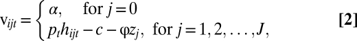
We assume that the ’s are an independent and identically distributed Type I Extreme Value. These errors can be thought of as profit shocks and could be positive or negative for a given individual, time, and location. The deterministic portion of returns from not fishing is the value of the nonfishery alternative (α), which could reflect the value of leisure, wages from other employment, or net earnings from another fishery that is unconnected to the J fishing sites. The deterministic portion of the fishing alternative is the profitability of fishing, which includes revenues from fishing (p_th_ijt), a fixed cost (c) of taking a trip (bait, ice, etc.), and travel cost ():

where h is individual expected harvest and p is price. Note that site-specific travel cost is the product of the distance from port to fishing ground z_j and the parameter ϕ, which can be thought of as fuel price. Suppose the catch function is the simple Schaefer (39) form:

where q is catchability, and E takes on a value of 1 if the site is chosen and 0 otherwise. Note that the results hold for a more general catch function as long as catch is monotonically increasing in stock and catchability. In this formulation, random variation in catches could also be the source of the variability in profits. In the static random utility maximization (RUM) model (40), the individual selects the choice with the highest returns for each choice occasion. Although we model the long run, we are assuming that fishermen’s expectations are myopic over time. Recent research has built other expectations processes into the RUM framework (41); we leave investigating forward-looking processes to future research.

Without loss of generality, we assume that forming a reserve eliminates the Jth choice in the choice set. Substituting Eq. 3 and Eq. 2 into Eq. 1 and applying the RUM assumptions, we can express a fisherman’s short-run expected WTP to avoid forming a reserve as

where we assume the marginal utility of income is unity because we model fishermen as maximizing expected returns. This expression captures per period expected returns lost or gained as a result of the reserve.

By inspection of Eq. 4 (in particular the summation across J and J−1 sites), expected WTP is positive, because formation of a reserve necessarily leads to a short-run loss from an individual fishermen’s point of view. The size of the loss depends on the parameters or characteristics of the fishery, which we explore in the short-run in Table 1.

We introduce heterogeneity in fishing skill by scaling catchability (q) on an individual basis by using a triangular distribution. Thus, a unit of effort for a high-skill fisherman catches more fish than a unit of effort for a low-skill fisherman. To aid in interpretation, we constrain catchability coefficients for each individual to be the same across space in the analyses of skill heterogeneity and in the dynamic simulations.

For the long-run analysis, we couple Eqs. 1– 4 with a dynamic population model of a three-site metapopulation (30). We match the time scale of fishing decisions to the annual scale of the biological dynamics. That is, fishermen decide whether and where to fish, the biology of the system updates, and then fishermen reassess the system and decide whether and where to fish in the next year. The population dynamics at each site take the form

where j is the site, t is the time step, i is fishermen, and the per capita growth rate is assumed to be logistic 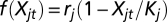with r_j and K_j denoting the intrinsic growth rate and carrying capacity, respectively, at site j. The dispersal function is represented by 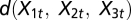and the different dispersal systems are nested by assumptions on the level of the dispersal rates (9). Population parameters, economic parameters, and the choice of a dispersal matrix define the baseline case explored in each simulation (SI Appendix A3, Table S1 and Table S2). Additional details are provided in SI Appendix A4.

References

- 1.Pauly D, et al. Towards sustainability in world fisheries. Nature. 2002;418:689–695. doi: 10.1038/nature01017. [DOI] [PubMed] [Google Scholar]
- 2.Worm B, et al. Impacts of biodiversity loss on ocean ecosystem services. Science. 2006;314:787–790. doi: 10.1126/science.1132294. [DOI] [PubMed] [Google Scholar]
- 3.Bernstein B, Iudicello S, Stringer C. Lessons learned from recent marine protected area designations in the United States. Report for The National Marine Protected Area Center (NOAA). National Fisheries Conservation Center, Ojai, CA; 2004. p. 91. [Google Scholar]
- 4.Bacher D. Senate majority leader calls for oversight hearing on MLPA process. In: Greenwald D, editor. California Progress Report. San Mateo, CA: CFC Education Foundation; 2009. [Google Scholar]
- 5.Turner M, Weninger Q. Meetings with costly participation: An empirical analysis. Rev Econ Stud. 2005;72:247–268. [Google Scholar]
- 6.Holland DS, Brazee RJ. Marine reserves for fisheries management. Mar Resour Econ. 1996;11:157–171. [Google Scholar]
- 7.Hannesson R. Marine reserves: What will they accomplish? Mar Resour Econ. 1998;13:159–170. [Google Scholar]
- 8.Pezzey JCV, Roberts CM, Urdal BT. A simple bioeconomic model of a marine reserve. Ecol Econ. 2000;33:77–91. [Google Scholar]
- 9.Sanchirico JN, Wilen JE. A bioeconomic model of marine reserve creation. J Environ Econ Manage. 2001;42:257–276. [Google Scholar]
- 10.Smith MD, Wilen JE. Economic impacts of marine reserves: The importance of spatial behavior. J Environ Econ Manage. 2003;46:183–206. [Google Scholar]
- 11.Wilen JE, Smith MD, Lockwood D, Botsford LW. Avoiding surprises: Incorporating fisherman behavior into management models. Bull Mar Sci. 2002;70:553–575. [Google Scholar]
- 12.Micheli F, Halpern BS, Botsford LW, Warner RR. Trajectories and correlates of community change in no-take marine reserves. Ecol Appl. 2004;14:1709–1723. [Google Scholar]
- 13.Abesamis RA, Russ GR. Density-dependent spillover from a marine reserve: Long-term evidence. Ecol Appl. 2005;15:1798–1812. [Google Scholar]
- 14.McClanahan TR, Mangi S. Spillover of exploitable fishes from a marine park and its effect on the adjacent fishery. Ecol Appl. 2000;10:1792–1805. [Google Scholar]
- 15.Broad K, Sanchirico JN. Local perspectives on marine reserve creation in the Bahamas. Ocean Coast Manage. 2008;51:763–771. [Google Scholar]
- 16.Bockstael NE, Opaluch JJ. Discrete modelling of supply response under uncertainty: The case of the fishery. J Environ Econ Manage. 1983;10:125–137. [Google Scholar]
- 17.Eales J, Wilen JE. An examination of fishing location choice in the pink shrimp fishery. Mar Resour Econ. 1986;2:331–351. [Google Scholar]
- 18.Curtis R, Hicks RL. The cost of sea turtle preservation: The case of Hawaii’s pelagic longliners. Am J Agric Econ. 2000;82:1191–1197. [Google Scholar]
- 19.Mistiaen JA, Strand IE. Supply response under uncertainty with heterogeneous risk preferences: Location choice in longline fishing. Am J Agric Econ. 2000;82:1184–1190. [Google Scholar]
- 20.Smith MD. Two econometric approaches for predicting the spatial behavior of renewable resource harvesters. Land Econ. 2002;78:522–538. [Google Scholar]
- 21.Haynie A, Layton DF. An expected profit model for monetizing fishing location choices. J Environ Econ Manage. 2009 [Google Scholar]
- 22.Holland D, Sutinen JG. Location choice in the New England trawl fisheries: Old habits die hard. Land Econ. 2002;76:133–149. [Google Scholar]
- 23.Valcic B. Spatial policy and the behavior of fishermen. Mar Policy. 2009;33:215–222. [Google Scholar]
- 24.Smith MD. State dependence and heterogeneity in fishing location choice. J Environ Econ Manage. 2005;50:319–340. [Google Scholar]
- 25.Hilborn R, et al. When can marine reserves improve fisheries management? Ocean Coast Manage. 2004;47:197–205. [Google Scholar]
- 26.Botsford LW, Micheli F, Hastings A. Principles for the design of marine reserves. Ecol Appl. 2003;13:25–31. [Google Scholar]
- 27.Smith MD, Wilen JE. Marine reserves with endogenous ports: Empirical bioeconomics of the California sea urchin fishery. Mar Resour Econ. 2004;19:85–112. [Google Scholar]
- 28.Holland DS. A bioeconomic model of marine sanctuaries on Georges Bank. Can J Fish Aquat Sci. 2000;57:1307–1319. [Google Scholar]
- 29.Kahui V, Alexander WRJ. A bioeconomic analysis of marine reserves for paua (abalone) management at Stewart Island, New Zealand. Environ Resour Econ. 2008;40:339–367. [Google Scholar]
- 30.Sanchirico JN. Additivity properties in metapopulation models: Implications for the assessment of marine reserves. J Environ Econ Manage. 2005;49:1–25. [Google Scholar]
- 31.Smith MD, Zhang J, Coleman FC. Effectiveness of marine reserves for large-scale fisheries management. Can J Fish Aquat Sci. 2006;63:153–164. [Google Scholar]
- 32.Sanchirico JN. Designing a cost-effective marine reserve network: A bioeconomic metapopulation analysis. Mar Resour Econ. 2004;19:46–63. [Google Scholar]
- 33.Sanchirico JN, Wilen JE. The impacts of marine reserves on limited-entry fisheries. Nat Resour Model. 2002;15:380–400. [Google Scholar]
- 34.Murawski SA, Brown R, Lai HL, Rago PJ, Hendrickson L. Large-scale closed areas as a fishery-management tool in temperate marine systems: The Georges Bank experience. Bull Mar Sci. 2000;66:775–798. [Google Scholar]
- 35.Cinner JE. Designing marine reserves to reflect local socioeconomic conditions: Lessons from long-enduring customary management systems. Coral Reefs. 2007;26:1035–1045. [Google Scholar]
- 36.Wilen JE. Why fisheries management fails: Treating symptoms rather than causes. Bull Mar Sci. 2006;78:529–546. [Google Scholar]
- 37.Grafton RQ, et al. Incentive-based approaches to sustainable fisheries. Can J Fish Aquat Sci. 2006;63:699–710. [Google Scholar]
- 38.Jones PJS. Equity, justice and power issues raised by no-take marine protected area proposals. Mar Policy. 2009;33:759–765. [Google Scholar]
- 39.Schaefer MB. Some considerations of population dynamics and economics in relation to management of marine fisheries. J Fish Res Board Can. 1957;14:669–681. [Google Scholar]
- 40.McFadden D. Conditional logit analysis of qualitative choice behavior. In: Zarembka P, editor. Frontiers in Econometrics. New York: Academic; 1974. [Google Scholar]
- 41.Hicks RL, Schnier KE. Eco-labeling and dolphin avoidance: A dynamic model of tuna fishing in the eastern tropical Pacific. J Environ Econ Manage. 2008;56:103–116. [Google Scholar]
Associated Data
This section collects any data citations, data availability statements, or supplementary materials included in this article.