A Kalman filtering approach to the representation of kinematic quantities by the hippocampal-entorhinal complex

Abstract

Several regions of the brain which represent kinematic quantities are grouped under a single state-estimator framework. A theoretic effort is made to predict the activity of each cell population as a function of time using a simple state estimator (the Kalman filter). Three brain regions are considered in detail: the parietal cortex (reaching cells), the hippocampus (place cells and head-direction cells), and the entorhinal cortex (grid cells). For the reaching cell and place cell examples, we compute the perceived probability distributions of objects in the environment as a function of the observations. For the grid cell example, we show that the elastic behavior of the grids observed in experiments arises naturally from the Kalman filter. To our knowledge, the application of a tensor Kalman filter to grid cells is completely novel.

Introduction

The encoding of space and time coordinates is a basic problem which the brain must solve. Multiple (perhaps most) brain regions are involved in this problem. At a basic level, primary sensory afferents must relay a topographic map from the mechanoreceptor sites to the primary somatosensory cortices. At a more abstract level, association cortices must build and update geometrically complex models of the environment to direct accurate behavior. Specific anatomic regions have been selected by experimentalists to study space–time reasoning. “Arm-reaching” neurons in the parietal cortex of primates have been used to study how visual cues are transformed from eye coordinates to arm coordinates (Ferraina et al. 1997). The inferior colliculus of the bat and ferret has been used as a model for time-interval coding (Ehrlich et al. 1997). The hippocampal-entorhinal complex (HEC) and its neighboring regions, in particular, contain a rich array of cells tuned to kinematic variables. These include place cells in the hippocampus, head-direction cells in the postsubiculum, and grid cells in the entorhinal cortex of rats (O’Keefe and Dostrovsky 1971; Taube et al. 1990; Hafting et al. 2005).

In each of the experimental models mentioned, computational models have been devised to predict how cells will fire when the animal is exposed to a stimulus oriented in space–time. Models for predicting cell activity for the reaching problem have been proposed by Cisek (2006) and Pouget and Snyder (2000). Particularly successful place cell models have been proposed by O’Keefe and Burgess (1996), Barry et al. (2006), and Balakrishnan et al. (1999); countless others exist. Notable models of entorhinal grids have been constructed by Fuhs and Touretzky (2006), Rolls et al. (2006), and Blair et al. (2007). Extensions of the theta phase precession theory for place cells and grid cells were given by Igarashi et al. (2007), Baker and Olds (2007), Wagatsuma and Yamaguchi (2007), and Takahashi et al. (2009). It is puzzling to note that the models mentioned differ from one brain region to the next, although the stimuli and task in question may be indistinguishable. Take the example of an animal reaching for an object in the environment. According to the parietal view, we might say that the animal transforms the object’s image on its retina from retinal to hand coordinates to facilitate reaching; each step in this transformation has been documented in the parietal cortex. From the hippocampal standpoint, we might argue that the hippocampus has a place cell anchored to the same object which “informs” the animal of its location. It follows that two simultaneous representations of the same object must exist. We would like to pose the question: which representation determines the animal’s reaching behavior? The natural answer is that both representations contribute; i.e., the two brain regions are working on the same calculation together. If this is the case, however, why does one need two different mathematical models to perform one calculation?

The simplest answer to this problem would be to suppose that all space–time calculations in the brain are carried out according to a set of common rules. If one could determine these rules, it would be unnecessary to build a new mathematical model to explain how each new brain region calculates space–time relations. Instead, one would have to figure out “which part” of the overall calculation the region in question was doing.

In this paper, we have attempted to group several of the brain functions just described under a common set of rules. The rules adopted correspond to those used by engineers to deal with the analogous problems in robotics (Gelb 1984; Smith et al. 1990). These rules have already been applied to the hippocampus in several important papers (Bousquet et al. 1999; Szita and Lorincz 2004). The author’s goal is to show that the same scheme can be applied with equal success to any brain region which represents space–time; we will outline this procedure in detail for the parietal cortex (reaching cells) and entorhinal cortex (grid cells). We will also revisit place cells with a somewhat different interpretation than that of Bousquet et al. (1999).

Assumptions of the Kalman Filter

The set of rules utilized in this paper will be the state update equations of the linear Kalman filter. This filter is useful for computations and experiments due to its simplicity. However, we do not wish to create the impression that the unity between the several problems presented would vanish if a more generalized set of rules were used. To this end, we will briefly review the series of assumptions which connect the Kalman filter to the basic rules of probability. Analogous arguments for fuzzy sets could be made by replacing probabilities with membership functions.

Given a sample space containing various events, we can define the unions and intersections of these events. A particular type of sample space arises if we consider a particular collection of mutually exclusive “states” at multiple time points. We will refer to the states contained within a given time point as a “frame.” In this type of space, the only non-zero conditional probabilities are between states at non-identical time points. If we further constrain the conditional probabilities to only involve states at adjacent time points (the Markov property), we obtain a Markov chain.

A Markov chain of particular value to the neuroscientist is the hidden Markov model (HMM), which is used to incorporate the effect of observations on the probability distribution of a hidden stochastic process. Denoting the initial state vector by the state transition probabilities by and the state emission probabilities by the probability of a given observations sequence in a HMM can be written as:

1a

A key assumption in the HMM is that the observations are independent of one another and of states outside the corresponding time point. This assumption is hard to justify experimentally. We find this to be a major limitation of the HMM, but the complexity of alternative formulations without this assumption appears prohibitive at this time.

Special Markov chains can be obtained by restricting the permitted types of state transitions. If the states considered are a lattice of cubes within a volume of space, we might permit only transitions between neighboring cubes. A random walk has this property. Letting these cubes shrink to infinitesimal dimensions, we obtain a random walk for continuous variables (a diffusion process). Nonlinear filters such as the Kolmogorov and Zakai equations, or linear filters such as the Kalman and Wiener filters, fall into this category (Gelb 1984).

We require the analogue of Eq. 1a for continuous variables to generate the Kalman filter. For the discrete-time case, the system transitions (or “control inputs”) and state emission probabilities (or “observations”) may be considered separately. For the system evolution model x(k) at time-step k,  we take the linear equation:

1b

Here a(k) and b(k) are model parameters which we will set equal to unity, u(k) is a control input variable, and w(k) indicates additive random noise. Similarly, for the linear observation model z(k) we let:

1c

Here c(k) is a model parameter which, again, will be set equal to unity. The term v(k) denotes additive random noise. The random variables w(k) and v(k) will be assumed continuous and normally distributed, with covariance matrices R(k) and Q(k), respectively.

Further discussion of these state equations may be found in Gelb (1984) or Dissanayake et al. (2001).

An important concept relating to the Kalman filter is the “frame.” As mentioned previously, by a frame we shall mean the probabilities of all states at a particular time point. Physically, we can relate a particular “state of knowledge” by the observer to each time point. In the diagrams provided throughout the paper, separate frames are represented by separate icons.

The uncertainty between frames

It is possible to classify state estimation problems by the number of frames of type B (brain) and W (external world) of a system. Namely, we can permit each subset to have one or multiple frames. This scheme yields 4 possibilities for B/W combinations: 1/1, 1/N, N/1, N/N. These combinations correspond to the 4 situations encountered by a brain when it represents the motion of extended bodies. We will list, for each, an experimental example:

• 1/1—the problem of representing one’s body position in space (modeled as point-like) relative to a perfectly known (or “very familiar”) environment. The example of place cells will be used.

• 1/N—the problem of representing body position in space relative to an imperfectly-known environment, or representing the relative positions of objects in the environment. Place cells, time cells, and head-direction cells are examples.

• N/1—the problem of representing the extended body of a subject (where uncertainties between sensors may exist). The reaching problem (studied in the parietal cortex) will be addressed.

• N/N—a generalized case of the preceding problems. We will not discuss it.

We will now examine each of these cases in detail. The reader is strongly encouraged to review Appendix Eqs. 31–34 at this time for a detailed overview of the methods used. Owing to the space required for a full description of these methods, we chose to omit them from the body of the text.

Body position relative to a perfectly known environment

General results

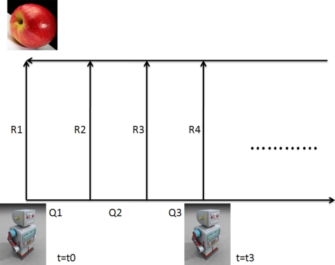
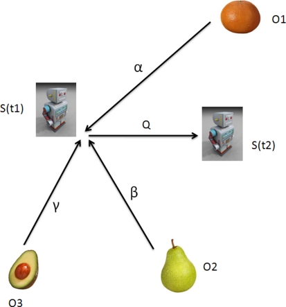
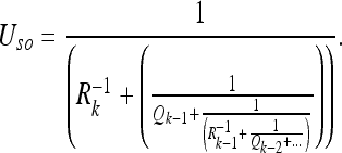
The directed acyclic graph (DAG) for the estimation problem 1/1 is shown in Fig. 1. This problem represents the most basic form of the Kalman filter; we will try to gain intuition for its properties in this section. A subject makes observations of a single non-subject frame (we will call it an object) while the subject performs a series of motions through space. The relative uncertainty U in the positions of the subject S and the object O, calculated according to Appendix Eqs. 31 and 33, is given in Eq. 34:

2a

Here Q_k and R_k represent the state evolution observation covariances, respectively, at time step k. The corresponding position estimates can be calculated according to the Kalman filter equations as shown in (34). Since the uncertainty expressions govern the state evolution, however, we will only give U explicitly.

Fig. 1.

A subject makes alternating observations (with covariances R_k) and control inputs (with covariances Q_k). Evaluating the circuit resistance between the subject at time step k and the object yields Eq. 2a

The expression 2a agrees with our intuition about how “certain” our subject (say, a rat) is of the position of a particular object relative to its body. If the rat makes a perfect observation R_k = 0, then we find U = R_k = 0. Similarly, if a very inaccurate observation R_k → ∞ is made, it follows that U_n = U_n−1; the new observation makes no impact on the rat’s state estimate.

In general, a rat will never be “completely certain” or “completely uncertain” of its position in a familiar environment. Rather, the rat’s uncertainty will tend to fluctuate within some finite range between the 2 extremes when the number of observations becomes large. We would like to estimate this range. To do this, we begin by setting all the terms Q_i and R_i equal in 2a. We then take the limit of 2a when k → ∞:

2b

If we let Q_max, R_max denote the poorest (least precise) observation and the poorest control input, and let Q_min, R_min equal the best values for these quantities, we can insert these values in 2b to get a “maximum range” for the uncertainty. This is:

We see that U must remain finite and nonzero if Q_max, R_max and Q_min, R_min are all finite.

If the relative positions of all objects in an extended environment are known with certainty (see IIIB2), then Eq. 2a holds for the uncertainty of the rat with respect to any object in the room. That is:

In other words: if all the objects O₁, O₂, … O_n are equally “observable,” i.e.

the rat gets the same information from observing different objects as it does from observing only one object! We may as well call this common uncertainty “the uncertainty of the rat with respect to the room.” This is precisely the relation which hippocampal “place” cells are believed to represent. Consequently, we should be able to make predictions about place cell fields using our model. We shall do this in the next section.

Let us consider other special cases of Eq. 2a. In the limit, if the rat could drive U to zero, a precise point in the rat’s body could be represented with respect to the world (to be discussed further for the case N/1). This implies that place cell fields can (in principle) become arbitrarily point-like in space, provided observations become suitably accurate. The best way for the rat to do this would be to minimize its internal sources of error Q; for instance, it might choose to remain roughly stationary. Setting Q = 0 in Eq. 2a, we have:

3

For k roughly identical observations R this reduces to U = R/k.

Conversely, imagine that a rat at a particular moment knows its position with uncertainty U = U₀. If we then deprive the rat of further landmark information (perhaps by turning off the lights), Eq. 2a gives (with R_i = 0 and k control inputs):

This situation represents “pure path integration” by the rat, and results in progressive enlargement of the uncertainty ellipsoid (Dissanayake et al. 2001). If we measured the summed activity of a population of place cells at a particular time (we assume the distribution is Gaussian), we might expect the distribution’s volume to increase in this case. We are not aware of experiments which have demonstrated such a phenomenon, although experiments on blind rats have been conducted (see, for instance, Save et al. 1998). This implies that the “position estimate of the rat with respect to a particular landmark at a particular time” and a “place field” are not equivalent quantities; we discuss a more likely relationship between them next.

Predictions for place cell fields

Thus far, we have demonstrated that a state-estimator satisfies our intuitive notions regarding that quantity which may be called “the uncertainty of the subject with respect to a landmark.” We now need to show that this quantity actually agrees with what is known about place cells in the HEC. To make this leap, we will need to assume a relationship between the firing-rate F of a place cell population (or PCP) X at time t and the probability that the rat is at the position x:

Here denotes a normal distribution with mean μ and variance σ². To begin with, we need to take into account that experiments have typically considered the sum of all action potentials for a given PCP over some time interval As we know, the rat’s state estimate (according to the Kalman filter) will generally not agree with the rat’s true position unless the rat knows its position relative to all landmarks with perfect certainty. This implies that a given PCP will not achieve peak firing at precisely the same location with each visit. Thus, the “firing field” of a PCP which is measured experimentally is actually the sum of multiple, distinct position estimates made at various times:

Here Thus, a given place field (according to the usual experimental definition) will consist not of a single normal distribution, but rather a sum of such distributions.

We now wish to predict some of the place cell fields observed by O’Keefe and Burgess (1996). This study examined how place fields changed when a familiar rectangular enclosure of dimensions l × w was deformed to a new configuration l′ × w′. To initiate the Kalman filter, we will make the following assumptions:

A1 The only landmarks are the corners of the enclosure. The positions of the corners serve to specify the dimensions of the enclosure completely.

A2 The rat possesses no memory for observations made after the deformation. This is equivalent to the requirement that Q → ∞ in Eq. 2a for all control inputs after the deformation. The consequence of this requirement is that the rat’s state estimate at any moment will only depend on the information available at that moment and the information acquired before the deformation.

A3 The estimates for the length l and width w of the enclosure are uncorrelated.

With these assumptions, we initiate the Kalman filter. At any moment the rat will observe a certain combination of corners. If the observed corners have a configuration identical to that of the undeformed enclosure, the PCP will fire identically in the deformed/undeformed rooms (relative to the observed landmarks). Conversely, if the relative orientations of the observed corners have changed, the rat will need to generate some new estimate of its position relative to them. Since there are only 4 corners total, we can easily tabulate all possible observations. We must keep in mind that the state estimates we write down are actually averages, since each individual observation is subject to random error.

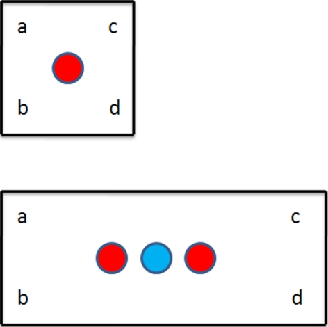
Let us take first a square box w × w which is deformed to a rectangle w × l, as shown in Fig. 2 (top panel). Tabulating all possible observations, we obtain 3 possible state estimates.

Table 1.

Three possible state estimates are generated from all possible corner combinations

Corners observed	State estimate	(Corners cont’d)	(State cont’d)
None	None	bc	3
a	1	bd	3
b	1	cd	2
c	2	abc	3
d	2	abd	3
ab	1	acd	3
ac	3	bcd	3
ad	3	abcd	3

Fig. 2.

A rectangular enclosure l × w is stretched to new dimensions l′ × w. Three different views of corner combinations are possible; only one takes into account the new dimensions. The color red denotes positions where the place cell in the top panel will continue to fire in the bottom panel. See Table 1 and Eq. 4b

Thus, if the “place field” in the square box was Gaussian, the field in the rectangle will be (setting 1 = ab, 2 = cd, 3 = abcd):

4a

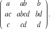
This three-peaked field is shown in Fig. 2. We write the labels for the rectangle in Fig. 2 (lower panel) in matrix form:

4b

We would expect the Gaussians in brackets (Eq. 4a) to be of greater amplitude since their variances will be smaller (i.e., the PCP will fire more vigorously for corner configurations which are not deformed than for those which have undergone deformation). This result is in agreement with the experimental results obtained by O’Keefe and Burgess; in fact, it also accounts for the observed peak which did not appear in the model they developed (O’Keefe and Burgess 1996). It is worthy of note that if we permitted the rat some post-deformation memory, the peaks and would gradually migrate toward This accounts for the “blurring” observed between the 3 peaks in Fig. 2a (upper right panel) of O’Keefe and Burgess’s paper (1996).

We give the corresponding expression for a rectangle l × w which is deformed to a rectangle l′ × w′. For convenience, we label the distinct Gaussian terms with respect to the corners:

5a

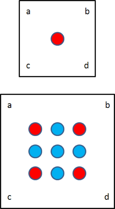
Here we have set for brevity. Again, we see that the terms in brackets correspond to the peaks predicted by the model of O’Keefe and Burgess; these peaks correspond to corner views which appear identical. This place field is shown in Fig. 3. We give the corresponding matrix form of the state estimates for the large square (as in the lower panel of Fig. 3):

5b

The reader can verify that all other corner combinations yield one of the state estimates listed here. In their paper, O’Keefe and Burgess (1996) presented the bracketed terms of P(x) in the form:

6

Although these results are promising, we were unable to predict some of the firing-fields found by O’Keefe and Burgess (1996) by inspection alone. This difficulty is not unexpected, as the fields should be highly dependent on the particular observation programmes (which were not available to the author). We would propose the method of robotic simulation (pioneered by Burgess et al. 1997) as best suited to this challenge: if one could record the rat’s observations as a function of time and then enact the same observation programme using a robot, it might be possible to duplicate the fields with great precision. For numerical simulations of time-dependent place field migration using the Kalman filter, the reader may refer to the study by Bousquet et al. (1999).

Fig. 3.

A rectangular enclosure Q_h is stretched to new dimensions l′ × w′. Nine different views of corner combinations are possible; five take into account the new dimensions. See Eq. 5b

The reader will note that we are not the first to posit a relationship between place fields and Kalman filtering. A previous effort of this kind was made by Balakrishnan et al. (1999). The formulation utilized by these authors differed from ours in that they considered a system state vector which included each PCP field explicitly. This differs from our interpretation, where the collective activity of the PCP is identical to the rat’s state estimate of its position at a given time; as such, place fields need not appear explicitly in the state vector. We cannot see a way to predict the non-Gaussian geometry of place fields using the scheme suggested by this group (Balakrishnan et al. 1999). Nevertheless, their work represents a major advance in our understanding of the HEC as a state-estimator.

Body position relative to an imperfectly-known environment

We can consider 2 types of uncertainties for the problem 1/N. First, we have the uncertainty of the observer S with respect to all the objects O₁, O₂, … O_n, which will call the interaction uncertainty:

Conversely, we can define the uncertainty of the objects independently of the observer, which we will refer to as the mapping uncertainty:

We will find U_int and U_map first for the most general (uncertain) case and then for the limiting (certain) case.

General case

Upper bound for uncertainty

For the general case of the uncertainty U_12…n between N frames, we can only establish an upper bound for the determinant according to the formula (Gersho and Gray 1992):

Writing the uncertainty for N frames evaluated with respect to the frame i, we have:

7

Here U_ij denotes the relative uncertainty of the frames i and j. Using the general formula 7, we can write the upper bound for the interaction uncertainty as:

8

That is, the subject’s uncertainty with respect to all the objects cannot exceed the product of the individual subject-object uncertainties. Similarly, we can write the upper bound for the mapping uncertainty as:

9

That is, the uncertainty of the all the objects with respect to one another cannot exceed the product of all pairings with the reference object. The formulas 8 and 9 provide a powerful means of approximation when the covariance matrix becomes large and difficult to evaluate.

The uncertainties for zero process noise

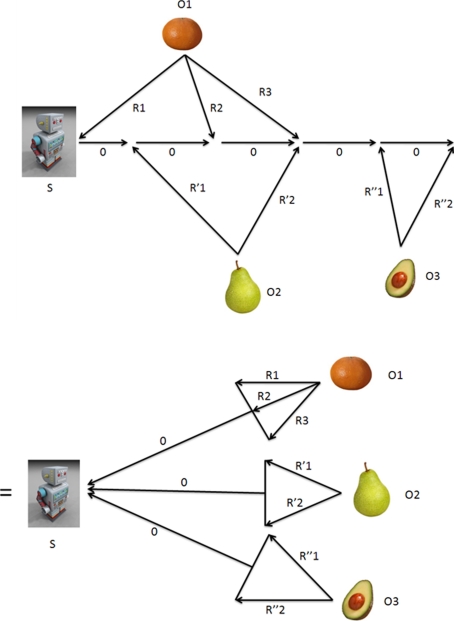
If we set the process noise Q equal to zero, we can find the uncertainty for N objects explicitly. We refer to Fig. 4 (top panel). We can see that the circuit for multiple observations of each object can be drawn in a form identical to that for one observation of each object (bottom panel). We will find the uncertainties for 3 objects; the results can be easily extended. To simplify the expressions, we will set:

We find the uncertainty between the 3 objects and the observer to be:

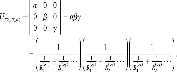10

This is the interaction uncertainty U_int defined previously. Conversely, we can evaluate the uncertainty between the 3 objects:

11

This is the mapping uncertainty U_map. Extending these formulas to 4 objects gives:

12

Fig. 4.

(Top panel) A subject makes observations (with covariances R_k for object 1, for object 2, and for object 3) and control inputs (with covariances all zero); numbers denote time steps. (Bottom panel) This circuit can be rearranged to yield a simpler one; the result is Eq. 10

The quantity U_int, as expected, goes to zero when a perfect observation of any object is made (when the relative uncertainty between the subject and one object becomes zero). As noted in A3, to preserve the information about the remaining N − 1 objects we must drop the zero terms from the determinant. For instance, a perfect observation of one of 4 objects will require the transition:

By contrast, the quantity U_map does not go to zero following a perfect observation. To make this quantity go to zero, we must make the relative uncertainty between 2 of the objects zero. This highlights the fact that U_map is an observer-independent quantity.

We can illustrate the objectivity of U_map in another way. Suppose that, after observing three objects as before, the observer executes a control input Q (Fig. 5). The interaction uncertainty will now be:

13

The mapping uncertainty U_map will, however, remain unchanged. This reflects the fact that the control input Q has not changed the observer’s knowledge about the relative position of the three objects. Note also that U_map did not increase; this is a general property of U_map we will explore in the next section.

Fig. 5.

The bottom panel of Fig. 4 is simplified and redrawn on the left. We then add a control input which transitions the observer from state 1 to state 2. See Eq. 13

Limiting case

Convergence and measurement conditions for the mapping uncertainty

Dissanayake et al. (2001) proved for the quantity U_map the following 2 properties, valid for arbitrary observations and control inputs in a static environment:

1. U_map is non-increasing.

2. If the number of observations n for each object increases without bound, then U_map approaches zero.

That is:

14

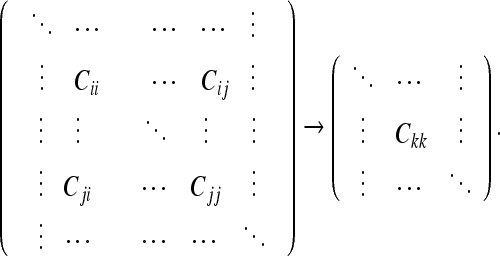
Since we might choose to evaluate the particular uncertainty U^(p)_map for any subset p of objects in our overall DAG, Dissanayake’s result can be applied to this subset as well. This allows us to “condense” the frames of p into a single frame:

The property (2) enables us to convert any multi-object observation problem into a single-object observation problem by achieving convergence in the sense 14. Once convergence between objects has been reached, Eq. 2a is sufficient to describe the subsequent Kalman filter dynamics. The asymptotic approach of the mapping uncertainty to zero was nicely demonstrated by Dissanayake et al. (2001) with an autonomous motor vehicle.

Equation 14 also permits us to state the conditions for which an experimenter can expect to measure a kinematic tuning in the brain (note that we use the terms “tuning” and “convergence” interchangeably here). These conditions are:

1. Subject observability If the world W is characterized by n continuous quantities q_i, a brain B may (in principle) acquire a tuning to any coordinate element of the form:

   15a

   Here we assume that a cell population’s tuning corresponds to the probability P(q₁, q₂, …q_n) of the coordinates q₁, q₂, …q_n for some physical process. Thus, the cell population’s tuning (or firing rate) dT for the coordinate element would be given by an expression of the form:

   

   Since the quantities q_i are characteristic of the physical world and not necessarily of the brain, however, only the m quantities (m ≤ n) which have converged according to 14 will appear in 15a. Thus, the converged tuning of B is given by:

   15b
2. Experimenter observability Of the quantities , only the s quantities (s ≤ m) which are expressly measured by the experimenter will appear in 15b. Thus, the observed tuning of B is given by:

   15c

   Condition (2) implies that the number of measured tunings of a cell cannot be greater than its true number of tunings. We now apply these conditions to the arbitrary motion of bodies in space (their kinematics).

Kinematic convergence

1. Space–time The most general tuning which the brain may have for kinematic quantities includes the time coordinate, position coordinates, and angular orientation of the body in question:

   16

   Note that the “tuning element” 16 is not a volume element which specifies not just position, but the complete kinematics of an oriented point in space and time. That is, 16 expresses convergence not for a static spatial distribution, but for a static event. By a static event, we mean an event which occurs identically (the relative space and time intervals are the same) for each trial. This definition agrees with our intuition; we know we can “become familiar” not only with consistent spatial distributions (positions of objects in a room) but also consistent events (the coordinates of a friend’s face each time he smiles). Nevertheless, the fact that the observer’s observations for a given trial of the static event are constrained requires us to prove that convergence is possible over multiple trials; we do this in 35.

   It would be possible to verify the tuning 16 experimentally by measuring the appropriate cortical region while an animal observed the relative orientations of 2 objects, with one chosen as the origin and the other as the point in phase space This experiment would be somewhat more challenging to perform than the usual “place cell” experiments, given the large number of degrees of freedom. To the author’s knowledge, a simulation of space–time convergence has not yet been performed. Its existence is entirely confirmed by Dissanayake’s result and our proof; however, the time course for convergence will generally be much longer than that for a static space.

2. Less general tunings We now consider cells which satisfy only a portion of the tunings in 16; that is, only some of the variables satisfy the condition (2). We will outline measurement conditions 15c such that

   It is easy to see that an infinite number of such “partial” tunings exist; this follows from the fact that an infinite number of “planes” of dimension N − 1 can be drawn in a “volume” of dimension N. We will consider only a few experimentally relevant examples here.

1. “Time” cells

Let us imagine some static event in which only the time coordinate converges. A good example would be an auditory pattern, where the only parameters of interest are the particular characteristics of the sound (e.g., intensity and pitch) and the times at which they occur. We could easily design an experiment exactly analogous to the usual “place field” experiments to test whether a rat’s “place” cells can also tune to time intervals. We would merely need to play the same auditory pattern (maybe a musical recording) repeatedly to a rat while measuring the same cortical cells. Instead of averaging firing-rates over all visits to a particular spatial location, we would average them over all trials of a particular note in the pattern. We would expect to find that different notes in the composition would be represented by different cells, just as in the spatial case. It is known already that cell in the inferior colliculus of the bat and ferret show time-interval tuning (Ehrlich et al. 1997); if the HEC serves a global memory role we should expect temporal tuning there as well.

2. “Place” cells

We can also imagine cells with a tuning consisting only of the spatial variables P(x, y, z). These are exemplified by the well-known “place” cells already discussed; it was recently verified by Jeffery et al. (2008) that place cell tunings extend to 3 dimensions. It is also known that there exist cells with approximately 2-dimensional tuning; entorhinal grid cells appear to obey this property (Jeffery et al. 2008). We see that in the context of the present theory, it is meaningless to speak of cells which represent strictly 2D or 3D space; rather, we speak of the degree of convergence (as expressed by 5) which a particular cortical region exhibits for a particular coordinate. The only reason entorhinal grid cells appear to represent the “2D space” of an explored surface is that the rat’s observation behavior selects objects on the floor as the most useful landmarks. If the rat were to explore a box in zero gravity (let’s assume the rat is still “stuck” to the walls), grid cells would likely adopt the normal coordinate vectors n_x, n_y of a given wall as the “most natural” coordinate tuning. Similarly, a rat exploring a curved surface would probably utilize normal coordinates in its entorhinal map.

Of course, we must remember that the observed “place” cells represent only the relationship between 2 particular frames: the rat and a landmark, summarized as <s, o₁> (where s denotes the subject and o₁ denotes the landmark). Since, from what has already been said, we should have cells that can represent any frame combination of the form <s, o₁, …o_n>, to find the other types of place cells we merely need to construct situations where 2 non-rat frames execute relative motion. For example, we could place an object in the box with the rat and compare the object’s position relative to the box with the rat’s cortical activity; we should find that the rat possesses “place” cells representing the object’s position (rather than its own). Specifically, we would expect the positions of the rat and the object to appear as 2 attractor bumps within the PCP.

3. “Head-direction” cells

Another possible partial tuning is that of the angular variables P(θ, ϕ). These are exemplified by the “head-direction” cells (Taube et al. 1990). All the comments made previously for “place” cells pertain to them as well.

The extended body (or extended brain)

We now need to address how state estimation can be carried out when the sensory apparatus of the observer consists of multiple frames. In doing so, we will resolve a paradox relating to “place” cell representation: which specific part of the rat’s body is represented by the place cell population? A similar issue arises in the study of the “reaching problem” in primates, since the brain appears to represent the various frames involved (hand, subject, and object) in various coordinate systems (Ferraina et al. 1997). We will focus on the case where the various sensors make measurements of a single non-observer frame (the problem N/1); this result can easily be extended to other cases.

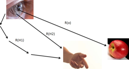
We can solve this type of problem by considering the various sensors as “point observers” which relay their observations to one another. As an example of this approach, consider the “reaching problem” illustrated in Fig. 6. We need to evaluate the uncertainty between the hand and the object U_ho, which is:

17

Here denotes the uncertainty of the object as viewed by the eye, R_h1 denotes the uncertainty of the hand as viewed by the eye, and R_h2 represents the uncertainty of the hand relative to the eye as measured by the proprioceptive (non-visual) system connecting the two.

Fig. 6.

The reaching problem at a single time point. is the uncertainty of the object image position on the retina, is the uncertainty of the hand image position on the retina, and R_h2 is the uncertainty of the hand relative to the eye through proprioception

We could transform between any 2 frames within the body in this way. In other words, a “place” cell population represents not a specific part of the body relative to an external landmark, but rather all parts of the body relative to the landmark with varying degrees of uncertainty.

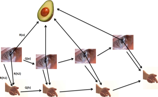
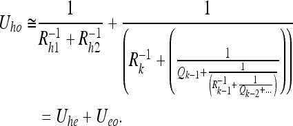
We can use the same approach to extend our Eq. 2a (the problem 1/1) to the case of an extended observer. The DAG for an observer consisting of 2 sensors is shown in Fig. 7. Control inputs to the hand and eye are assumed (for simplicity) to be independently generated, as shown. We cannot write down a general expression for the uncertainty U_ho; however, if we assume the control inputs Q_h → ∞, we can write:

18

Here we have neglected the index e for the observations R_e and control inputs Q_e in the in the second term to simplify the notation; U_he is the hand-eye uncertainty and U_eo is the eye-object uncertainty. We can see that the second term is simply Eq. 2a. Thus, the uncertainty between the hand and the target object is simply the point-observer uncertainty U_eo plus an additive term U_he under this approximation.

Fig. 7.

The reaching problem over multiple time points. In Eq. 18, we let Q_h approach infinity; Q_e and R_o are simply written as Q and R (k is the time step index) in Eq. 18

The principle outlined in this section can be easily tested in the HEC, preferably using primates. We might provide a monkey with a chessboard-sized “environment” containing various “landmarks” for spatial reference; the monkey would be encouraged to reach for objects placed at these various landmarks (analogous to “exploration” of the environment). We would then expect to find “place” cells which fired only when the monkey’s hand entered a particular part of this miniature environment. Thus, we find that place cells (hippocampus) and reaching cells (parietal cortex) encode very similar quantities.

Metric estimation

It was recently discovered that a population of cells in the HEC provide a spatial metric for the rat’s environment (Hafting et al. 2005). This metric is known as the “entorhinal grid.” More remarkably, it has also been shown that these grids are deformable; that is, the metric is not always Euclidean (Barry et al. 2007). In this section, we will show that the same estimation methods used in the previous section can be used to predict the dynamics of these grids. First, however, we must define some basic concepts of measure.

Preliminaries

Measures

Most of the day-to-day judgments we make about space intervals and time intervals are approximate. This imprecision arises from the fact that we usually do not possess precisely calibrated clocks or measuring-rods to establish the intervals in question. For example, a subject would usually not pull out a tape-measure to determine whether a parking-space was wide enough for his car. Instead, he would rely on comparisons of the desired interval with cues in the environment to make the judgment. This means that any physical relation in the environment might be employed as a measure.

It is equally clear from daily experience, however, that not all measures are created equal. If, for instance, a subject knew that the clocks in a particular building were notoriously unreliable, he would be better advised to consult a (more reliable) wristwatch if he wished to know the “time.” Examining this example a bit more carefully, we see that the establishment of a particular clock or measuring-rod as a “reliable” measure must always involve its comparison with another specified, reliable measure (preferably on multiple occasions). To use the previous example, if by comparing the clocks in a particular building with the watch on multiple occasions the subject should find them to consistently agree, he might as well simply consult the building clocks to determine the “time.”

In fact, we see that this procedure for establishing reliable measures is precisely analogous to Dissanayake’s convergence result, expressed in Eq. 14. We shall therefore use 14 to formally define what we shall mean by a standard of measure:

Definition: A standard of measure (or SOM) is one which has converged, in the sense of 14, relative to another SOM.

Thus, we see that physical relations which are both consistent and frequently observed will provide the “ideal” benchmarks for comparison. We also see that, if a particular measure has not converged, its use introduces error into the conclusions derived. This error can be quantified using the usual methods of state estimation.

The reader should note that, from here on, we will refer only to space in our discussion (for simplicity); the arguments all apply to time as well.

The subjective definition of space using measures

By displacing a physical object (or measure) through space, we may characterize the distance relations in any part of that space completely. That is, by a series of displacements of a given ruler, we can assign a distance between any 2 points within the volume under consideration. This collection of distance relations is called the metric for the space. If the measures used to define the metric are perfect, the metric estimate B (for “brain”) corresponds perfectly to the true metric W (for “world”) of the physical space. Since we live in an approximately Euclidean world, W is always Euclidean unless we define it otherwise (for instance, by “deforming” the environment from metric W to metric W′). Conversely, if some of the measures are imperfect, the metrics B and W will generally not coincide. This means that B will generally not be Euclidean.

It is important to realize that the metric estimate B,  like all the subjective quantities (internal to the brain) we have discussed in this paper, is defined exclusively in terms of the subject’s observations. The subject’s metric B is infinitely uncertain for any part of the true metric W which the subject has not measured using a measure. By making sufficiently detailed and concise measurements (using a SOM) of some part of W, on the other hand, the subject can make B approximate W as closely as he might desire.

We will assume that the metric estimate B corresponds exactly to the tessellating pattern of the entorhinal grids.

The metric tensor and generalized Kalman equations

Mathematically, there is no difference between “metric state estimation” and the ordinary state estimation procedures we employed in earlier sections of the paper. The distinction between the two cases instead arises from our choice of which parts of the system will be subjected to state estimation: in ordinary state estimation we assume an unbiased set of rulers to be provided (and not subject to state estimation), whereas in metric state estimation we do not make this assumption. In practice, however, it is useful to introduce a formal (mathematical) distinction as well. Since the metric intervals of interest are part of a continuum, they are more conveniently represented by utilizing the metric tensor g_ik. This entails a slightly different derivation of the Kalman state update equations (see “Extension of the vector Kalman filter to the metric tensor”) which leaves their basic structure intact. One can visualize the transition between the vector and tensor Kalman equations as analogous to the transition between a large number of springs and a continuum body in the theory of elasticity.

The metric tensor enables us to describe the infinitesimal distance relations at any given point of space. Since a subject cannot perform an infinite number of measurements, we must keep in mind that the subject’s state estimate can only approximate a continuum space. This approximation will improve as the number of measurements becomes large (as in the cases to be discussed here).

The transition of the Kalman equations from a vector to a metric description has a useful consequence: the “probability energy” u_ikP_iklmu_lm has the same form as the elastic energy of a deformed body (Extension of the vector Kalman filter to the metric tensor). If one overlooks the fact that “action at a distance” is prohibited in the linear elasticity theory (see “The relationship between the “probability” energy F and the energy for a linearly elastic body”), this analogy leads us to a useful mental picture of how “metric deformations” occur. Namely, we can picture each stage of the state estimation process as corresponding to the stretching or relaxing of a continuous elastic medium. The elastic analogy for the Kalman filter is crucial in that it parallels the “stretching” and “compression” properties observed in entorhinal grids; we will examine this more closely with the Barry et al. (2007) experiment.

Experience-dependent re-scaling of entorhinal grids

Simple example

Before applying the Kalman equations directly to the experiment by Barry et al. (2007), we will consider the simplest possible example of a “metric estimation cycle.” We take the situation shown in Fig. 8.

Fig. 8.

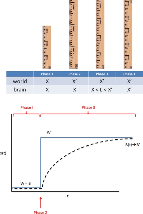
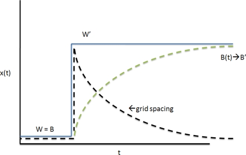
(Top panel) A ruler is noted to stretch from length X to X′. According to the ruler’s reading, however, its length is still X. To refute this, a second ruler is needed for comparison. If the second ruler is error-prone, we should take a weighted average of X and X′ (X < L < X′). (Bottom panel) The same process in continuous time

Phase 1

We imagine a rat observes a single object, a ruler X. Since no other objects exist in our simplified example, this ruler defines the rat’s concept of distance. This can be seen mathematically by noting that the rat’s estimate of the length l of the ruler X must be derived by measuring it relative to a set of measuring rods X, Y, … yielding length values (for the ruler X)x, y, … and associated errors σ_x, σ_y, … according to the general Kalman update formula 2a (which we shall simplify by setting the Q_i equal to zero):

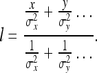19

In words, this equation says that the distance we denote “the length of the ruler X” is a weighted average of the lengths of X with respect to ruler X,  the ruler Y,  and so on. If only ruler X is available:

20

Thus, no matter what physical deformation the solitary ruler X should undergo, the rat will have no means for recognizing that any deformation has taken place. This fact, which runs counter to our experience, is of fundamental importance for understanding why entorhinal grids deform as they do.

Phase 2

The ruler X is now deformed to some new, physically different ruler X′ of length x′. Since the rat has no benchmark for comparison, it perceives no change in X′ from the structure of X; rather, its internal definition of length is deformed by a corresponding amount such that the perceived length of the ruler is unchanged:

To the experimenter, it will appear that the rat’s metric has instantaneously “stretched” upon observing the stretched ruler.

Phase 3

As the rat begins to explore its environment, it will discover other sensory cues. Mathematically, we might say that the rat discovers a new ruler Y with which to compare the ruler X′. Using our general equation, we derive the rat’s new estimate l₃ of the length of ruler X′ by comparison of the two rulers:

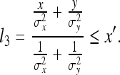21

If (as a special case) ruler Y is believed to be perfectly accurate (σ_y = 0):

That is, the rat discards the length of ruler X′ relative to itself and instead considers only the length of X′ relative to Y. If Y is in fact perfectly accurate (i.e., its length is always the same when it is observed), then:

As long as no perfect rulers exist, however, the rat’s estimate of the length of X′ can only approach its true value x′ asymptotically (on average). For instance, if all rulers have the same variance σ, then our general expression goes into:

22

Since x is the biased length of X′, we see that x < l < x′. This limiting behavior of the length estimate at (or near) its true value corresponds with our common-sense notion that lengths in an environment rich in sensory cues can be determined to a high level of accuracy. In this manner, we return to Phase 1.

Simulation of the Barry et al. (2007) experiment

We now consider the experiment of Barry et al. (2007) in detail. In these experiments, a rectangular box was deformed from a configuration l × w to a configuration l′ × w′. For simplicity, we consider the case where a square l × w is deformed to a rectangle l × w, with l > w. As in our earlier discussion of place cells, we will make certain assumptions.

A1 The rat’s estimates of l and w are uncorrelated.

A2 The corners of the enclosure provide the only landmarks for the rat. All state estimates by the rat are assumed rectangular.

A3 The structure constants E(u_iku_lm) have a form identical to those for a linearly elastic, isotropic body (see “The special case of an isotropic body” and “The relationship between the “probability” energy F and the energy for a linearly elastic body”).

Phase 1

The rat is permitted to become familiar with the rectangle, such that a Euclidean metric is established by the entorhinal grid. This metric is given by:

It is important to note that, by definition, the metric of a familiar environment is always Euclidean. This is a simple consequence of the fact that physical world is itself Euclidean.

Phase 2

The square w × w is deformed to the rectangle l × w in the rat’s absence, and the rat is returned to the rectangle. When the rat first views the dimension l of the rectangle, it concludes that the length of the rectangle is still w (since, initially, no external benchmark for comparison exists). The entorhinal grid then “stretches” along the long axis of the box. We can determine the resulting grid spacing m_ik with the help of the equation in “Relationship between the metric estimate and the spacing of entorhinal grids” (see Fig. 9):

23

That is, the rat’s grid spacing m_ik deforms by the same amount as the enclosure’s “physical” or “objective” metric does. We can compute this metric easily as:

24

Here a is some constant. The element of length for the deformed metric is:

25

It is not difficult to see the analogy between this initial deformation and the stretching of a rubber sheet secured at its boundaries to a template (identical in dimensions to our box). If we imagine that the metric intervals δ_ik were painted on the sheet prior to the deformation, the post-deformation metric would correspond to

Fig. 9.

The grid spacing is given not by the metric estimate, but rather its opposite (see Eq. 36). As the metric estimate expands, the grid spacing contracts

Phase 3

The rat, by moving about the box, obtains new sensory information which contradicts the non-Euclidean metric it obtained in Phase 2. Since the lengths of the two dimensions of the box have been assumed uncorrelated, the time-dependent “contraction” of the entorhinal grid reduces to a one-dimensional problem. In general, we need to solve the one-dimensional form of Eq. 19 in “Kinetics of the spatial metric” to determine the metric. This equation has an exponential family of solutions, as shown in “Kinetics of the spatial metric”. However, for large times after the deformation we can approximately describe the deformation by Eq. 21 in “Kinetics of the spatial metric”. The grid spacing then becomes approximately:

26

Here a and b are constants. For t = 0, this agrees with the result found previously. As t → ∞, the metric attains limiting (Euclidean) form:

27

In this manner, we return to Phase 1. This “relaxation” phase is not unlike the relaxation of our stretched rubber sheet once the template is removed from it.

This exponential nature of the relaxation phase explains the curious fact, noted by Barry et al. (2007), that when a box w × l is compressed to a rectangle w′ × l′ by the experimenter, the rat’s grid spacing m_ik(t) undergoes a lesser degree of compression along the same axis. The experimenters were not aware that the rat’s metric estimate m_ik(t) changes exponentially during the first few minutes of rat exploration in the compressed environment. As we discussed previously for place cell fields, time averaging procedures are not strictly applicable to such time-varying brain states. In other words, time-averages were applied to a large part of Phase 1 (Fig. 8), thus obscuring the exponential behavior. If we wish to capture the entorhinal grid spacing m_ik(t) at its complete compression stage (t = 0), we must average over only the very first few seconds of Phase 1 in Fig. 8. In general, smaller time windows will yield a more accurate description of entorhinal grid kinetics (Fig. 9).

In conclusion of our simulation, we note that a numerical simulation is of critical importance for determine whether the more complex “elastic relaxations” predicted by our model agree with experiments. Of course, our equations also require the setting of several boundary conditions (e.g., the observation matrix) which will probably have to be determined empirically.

More generally, we must remember the limitations of the basis used by us. Equation 26 is an approximation of the Kalman filter. The Kalman filter is itself an approximation to the phenomena in question (as discussed in “Assumptions of the Kalman Filter”). We should expect our approximate models to break down for times very close to time zero. This “time zero crisis” can be solved only by a more generalized theory which our theory approximates.

Comments regarding the generalized equations in "Extension of the vector Kalman filter to the metric tensor" and "The special case of an isotropic body"

Structure of the deformed metric

The precise structure of the deformed metric is determined by minimizing the energy:

28

Here we have set:

29

Here z_ik denotes the observed metric, H_iklm denotes the observation matrix, and u_ik represents the metric estimate. E(u_iku_lm) refers to the expected value of the square of the metric estimate. The origin of these expressions is further discussed in “Extension of the vector Kalman filter to the metric tensor”. Using 28, we can understand the deformation in an intuitive way. For instance, the metric within a familiar object (a near-SOM) will be expected to remain the same:

Consequently, a deformation of this object will make large contribution to the energy (the ratio 28 will be very large). The subject would be very “surprised” if the familiar object were to change its shape. In analogy with linear elasticity, a familiar object constitutes a “rigid body.” Conversely, if some part of the environment W₁ has received very few observations, the error associated with its metric (relative to the metric of any other part W₂, where W₁ may equal W₂) is very large:

Consequently, we can drop all terms containing W₁ in 28 since their contribution to the energy is zero anyway. Recalling our earlier discussion of entorhinal grids in IIB2b, we see that this explains why a rat exploring a 2D service constructs a nearly-2D metric for the environment. If we assume that the metric correlations E(u_iku_lm) are constrained to infinitely-near points in space (see “The relationship between the “probability” energy F and the energy for a linearly elastic body”), the “deformation of entorhinal grids” reduces exactly to the deformation of a 2D elastic sheet! By testing entorhinal grid deformation for rooms of various starting/ending geometries, this “elastic sheet” hypothesis might be put to the test. The corresponding equations can be derived as specializations of those already presented.

Extension to space–time

All the results we have cited here for space can be applied to space–time. Since the deformation process described here is time-dependent, however, it is easy to see that the time dimension imposes a constraint on the system observability. This constraint functions the same way a constraint on the observation of spatial variables of W′ would (previous example).

Discussion and conclusions

In the first section of the paper, the vector Kalman filter (KF) was applied to hippocampal place cells, parietal reach cells, and several other cell types in brief. It was shown that place cell populations most likely represent the relative uncertainty between the subject’s body position and a particular object in the external environment. It was demonstrated that place cell fields can be best reconciled with the KF (which requires Gaussian probability distributions) by making the assumption that the time bins in present experiments are too large to capture the instantaneous population activity. A simulation to verify this claim is critical to our assertion (in the introduction) that space–time computations are performed by a common set of rules throughout the brain.

The author then considered the problem of how maps of the external environment are actually formed (the case 1/N). Neither the case 1/1 nor the case N/1 addresses this problem. This problem is most important when a subject is first placed in a new environment, and creates great difficulties for the experimenter due to the complexity of the input data. It was shown by us that the computational demands on the subject are also considerable during this period, but can be reduced by minimizing control inputs on the part of the subject. We then presented Dissanayake et al. (2001) convergence result for a static environment, which proves that a subject can build a perfect (or converged) map of the environment from imperfect control inputs and observations. This result was used to show that the brain can acquire any kinematic tuning. Specific examples of place cells, time cells, and head-direction cells were mentioned. If we are correct in considering all these cells to share the same computational apparatus, they should also share the well-known probability distributions and time course of the KF.

For the case N/1, the parietal reaching problem was considered, and it was shown that this problem is just a variant of the place cell problem when the KF is applied. This fits with the intuitive notion, stated in the introduction, that these two problems are physically the same.

In the second section of the paper, the KF was further applied to the grid cells of the entorhinal cortex. The vector KF was reformulated so that it applied to tensor quantities; this development was necessary since the grid cells encode a dense array of environmental cues which is better accommodated by a spatial metric than a position vector. The update expressions for the tensor KF are closely analogous to the deformation expressions for an elastic body. The significance of this analogy can be found in the experiment of Barry et al. (2007), which demonstrated that entorhinal grids “stretch” and “compress” when a familiar environment is deformed. The equations presented are consistent with experience; for example, if a room is deformed in a rat’s absence, the dimensions of familiar objects in the room will change minimally even as the rat observes the deformed room boundaries. It is expected that a KF interpretation will be particularly fertile for future experiments in this area of research.

The major limitions of the approach adopted here are (1) the assumptions used to derive the KF (discussed earlier) and (2) the need for further implementation and simulation of the stated results. The theoretic results presented in the paper have been expressed in single-variable form (without matrices) and do not include the observation/state transition matrices explicitly. The Kalman filter is also rarely implemented in the “pure” form used here, since the covariance matrix rapidly becomes large in complex environments. A more important question is of how the various constants and parameters in the KF equations should be assigned to yield meaningful predictions about neural population activity, given information about the subject and environment. This question must be addressed partly by parameter-fitting with experimental data and partly by a search for the deeper theory which ours approximates. In some cases (as for place cells) animal experiments may be less useful than robotic simulations.

Appendix

State evolution and observation equations

For the system evolution model x(k), we take:

30

Here a(k) and b(k) are model parameters which we will set equal to unity, u(k) is a control input variable, and w(k) indicates additive random noise. Similarly, for the observation model z(k) we let:

31

Here is a model parameter which, again, will be set equal to unity. The term v(k) denotes additive random noise. The random variables w(k) and v(k) will be assumed continuous and normally distributed.

Further discussion of these state equations may be found in Gelb (1984) or Dissanayake et al. (2001).

Propagation of uncertainty for continuous, normally distributed (CND) random variables

In the following, we will make use of the following 2 identities for CND random variables:

(1) If Z = X + Y, where and X and Y are independent, then:

32

(2) If P(Z) = P(X)P(Y),  where P(X) and P(Y) are as before, then:

33

Since we have defined the state update x(k) as the sum of CND variables x(k − 1) and u(k), we can write:

Equation 32 then holds for x(n). If we have two independent sources of information X and Y about a given frame, then Eq. 33 enables us to combine this information. As the Eq. 32 demonstrates, we have for a series of control inputs the following variance expression (R_i = σ²_i):

34

Similarly, for a fusion of a series of independent observations of a particular parameter, we have from Eq. 33:

35

The rules 34 and 35 constitute what is called the circuit analogy for combination of variances (or circuit analogy). Thus, Kalman state transition diagrams can be conveniently reduced using the familiar rules of circuit reduction. A more thorough discussion of the circuit analogy is presented in Smith et al. (1990).

The uncertainty U

The invariants of an arbitrary matrix C_ij are given by a basic formula from linear algebra (Shilov 1977):

Of these invariants, we use the determinant (following the practice of Dissanayake et al. 2001) as our measure of “uncertainty” for 2 reasons:

1. Evaluating the determinant does not require us to determine the eigenvalues of the matrix C_ij.

2. The determinant has a direct relationship to the “volume of the uncertainty ellipsoid” (Dissanayake et al. 2001) of the normal probability distribution:

This can be seen from the normalization condition:

This gives us the non-normalized volume V of the distribution:

Since V and C are simply increasing functions of one another, we shall use the determinant rather than V itself to simplify matters. We shall refer to the determinant as the uncertainty, or U.

The determinant’s significance as the volume of the uncertainty ellipsoid has an important implication. If we let the relationship between any 2 frames be known with certainty, the determinant will go to zero. This is analogous to the collapse of an N-dimensional object to an (N − 1)-dimensional object. This means that a zero value for the determinant does not imply that the relationships between all frames are known with certainty. To preserve the information about the other non-zero relationships following a collapse, we must consider the (N − 1)-dimensional determinant.

Evaluation of the terms of the covariance matrix (CM)

Procedure

The circuit analogy can be used to evaluate the CM for any set of frames in a given DAG. We now provide a simple procedure for doing this.

First, we choose any subset of M frames (from the complete set of N frames contained in a given DAG, so that M ≤ N) whose relative uncertainty U we wish to evaluate. We specify this subset by its CM:

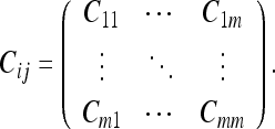Second, we choose one of the M frames in the CM as a frame of reference (FOR). Since the form of the CM will depend on which FOR we choose, we denote “the CM with respect to frame k” by C_ij/k. In our circuit analogy, we denote this by placing a current input at the FOR.

Third, we evaluate each term C_ij/k by placing current outputs at the frames i and j (maintaining k as our FOR). We call the frames i and j “frames of evaluation,” or FOEs. For the diagonal terms of the CM, we have one FOR and one FOE. The resistance through which we pass current (between the FOR and FOE) can be evaluated using Eqs. 34 and 35, exactly like an electrical resistance. For the cross-covariance terms, we have one FOR and 2 FOEs (one input and 2 outputs). We are interested in the common resistance of the circuit, which we define to be “the resistance through which the common current passes.” The common current is defined as “that part of the total current which is directed to both FOEs.” The common resistance can always be found by reducing the circuit (using Eqs. 34 and 35) to a Y-circuit. The resistance of the arm of the Y-circuit which carries current en route to both frames i and j is the common resistance; the resistances of the other 2 arms of the “Y” are omitted. In the CM calculated by the above procedure, the column and row corresponding to the FOR will be zero. We will always delete this column to avoid a zero value for the determinant; the nonzero minor of the complete CM is also invariant when we transform between any of the M FORs.

Fourth, we evaluate the determinant.

Example

We take as our example the DAG shown in Fig. 10. We will take as our covariance matrix the frames <2, 3, 4> or:

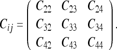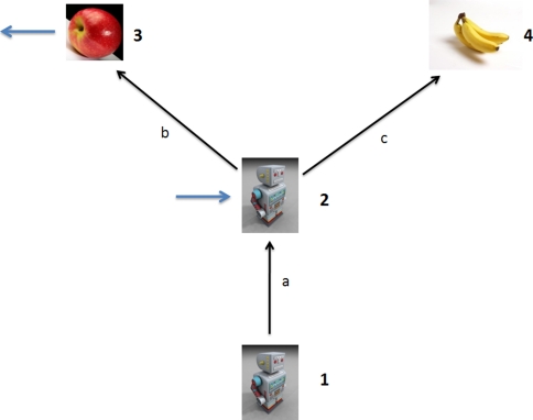
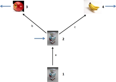
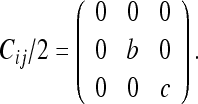
We will choose frame 2 as our FOR. We denote this in Fig. 10 by placing an input current at frame 2. We denote the CM with respect to frame 2 as C_ij/2. We will first evaluate the diagonal term C₃₃/2. To do this, we place an output current at the FOE (frame 3). We then evaluate the resistance between the input and output terminals (result shown below). We will now evaluate the cross-covariance term C₃₄/2. We place output current arrows at the 2 FOEs (frames 3 and 4), as shown in Fig. 11. We then determine the amount of current which passes to both FOEs from the FOR (zero in this case). Using the same procedure for the other terms, we obtain:

Eliminating the zero-valued row and column, we get:

We can carry out the same procedure by choosing frames 3 or 4 as our FOR; the results are:

It is easy to see that the determinant with respect to any frame of the CM is the same:

Fig. 10.

An input current at frame 2 and an output current at frame 3 are placed to determine C₃₃

Fig. 11.

Output currents at frames 3 and 4 are placed to determine the cross-covariance term C₃₄

Kalman filter

Using the state Eqs. 30 and 31 along with the propagation rule (32) and the combination rule (33), it is possible to describe a general algorithm for computing the most probable state of a changing system as new observations are made. This algorithm, when recursively formulated, is called the Kalman filter (KF). We will only summarize it here; the reader is directed to Gelb (1984) for a more complete discussion. The reader will note when comparing our expression with those in Gelb (1984) that we have set the model operators (the control input matrix and the observation matrix) equal to unity (see "State evolution and observationequations"). The KF defines the covariance update P₊ (with net pre-measurement covariance P_- and new measurement covariance R) as:

This is just Eq. 35. The corresponding state update μ₊ (with pre-measurement mean μ_- and measurement value z) is defined as:

This is just the mean update of Eq. 33.

The inter-measurement covariance extrapolation (based on the process model with update covariance Q) is:

This can be obtained from Eq. 30. Similarly, the inter-measurement state extrapolation is:

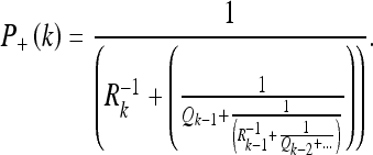
We give, for reference, the formulae for the mean and covariance after k applications of the Kalman filter. For the covariance, we have:

For the mean, we introduce the notation:

Setting μ_(1) = z₀, we can write the mean for any number of observations according to Table 2. This table is read as follows:

In this way, we can obtain the state estimate for an arbitrary number of observations.

Table 2.

Tabulated coefficients for the expansion of the mean estimate for the Kalman filter

	z0	z1	z2	z3	…
μ+ (1)	+1	−1	0	0	0
μ+ (2)	+2	+2	−2	0	0
μ+ (3)	+3	+3	+3	−3	0
μ+ (4)	+4	+4	+4	+4	−4
…	+5	+5	+5	+5	+5

The table can be expanded indefinitely by induction. See text for method of reading

Convergence for a static event

Let us consider a static event of dimensions We can slice this “space–time volume element” along the time axis into events of infinitesimal duration, for which the spatial coordinates vary only infinitesimally:

Since the values of the space coordinates do not change within each of these elements, we can obtain spatial convergence for any one of them simply by verifying that it is observed an infinite number of times, with each observation being independent of the others. This means that the observer must be free to choose a different observation programme for each trial of the event. If this independence holds, we have for trials (the upper index denotes the trial):

The terms in brackets on the second line are the converged spatial elements. This proves that a static event is completely observable.

Metric estimation

Extension of the vector Kalman filter to the metric tensor

The formal derivation of the vector Kalman filter (which we have referred to thus far in the paper) is presented in Gelb (1984). We shall only highlight the starting assumptions of its derivation.

The state estimate μ of the Kalman filter is derived by choosing the most probable value of the true state x, given the observations z. This means we wish to maximize the probability distribution:

36

Here and H denotes the observation matrix. This problem is equivalent to finding the extreme value of the exponent of 36, which we will call the “energy” F:

37a

To extend the vector Kalman filter to a 2-tensor, we simply need to write down the 2-tensor expression analogous to 37a. This is:

37b

Here we have set:

38

The terms in (38) have the same meanings as in 36. Following the procedure described in Gelb 1984, one obtains for the Kalman gain matrix:

39

Here we have set:

Recall that v_ik is the noise associated with the observation (see Eq. 31). Using (39), we can write the Kalman update from a prior covariance to a new covariance :

Here I_iklm = δ_ilδ_km is the unit 4-tensor. We can also write the state update from a prior metric estimate g⁻_ik to a new metric estimate :

The special case of an isotropic body

We will state the results of the previous section for the special case of an isotropic body. We first derive the energy F. By analogy with the theory of linear elasticity, we know that the P_iklm must take the form:

40

Inserting (40) in (37b), we have for the energy F:

41

Using the relations:

we can rewrite (41) in the more perspicuous form:

42

Here we have set:

We can also obtain the Kalman gain matrix K_iklm for the isotropic case. To simplify the result, we will set:

43

We will also separate the “pure compression” and “pure shear” terms of (40) as follows:

44

Similarly, we set:

45

Inserting (43, 44, and 45) in (39), we get:

46

The relationship between the “probability” energy F and the energy for a linearly elastic body

There exists an important difference between the metric deformations u_ik as they are utilized here and in the linear elasticity theory. To demonstrate this, we consider an undeformed elastic body divided into a large number of equal material volume elements, each with a particular position-vector x_l and metric g_ik tied to it.

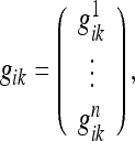
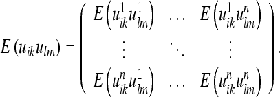
In the elasticity theory, the energy F associated with a material point is considered to be determined only by the metric deformation u_ik in its infinitesimal vicinity (well within the volume elements considered here), whereas in the present theory interactions between any set of material points may occur. Consequently, we must write:

47

In the special case where interactions are constrained to distances within the volume elements, the covariance matrix is reduced to its diagonal elements:

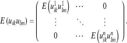The energy F = u_ikP_iklmu_lm in this case reduces to the form:

This is just the energy of an elastic body in its usual form.

Kinetics of the spatial metric

We now examine how the quantities u_ik must evolve over time in the continuous formulation. We will solve the problem for the vector Kalman filter and then generalize the result. The vector evolution is given by (Gelb 1984):

48

Here x is the true state of the system, μis the state estimate, F is the control input matrix, K is the Kalman gain matrix, H is the observation matrix, w is the process noise (and G its gain), and v is the observation noise.

If the rat has been observing the deformed environment for a long time, then the Wiener conditions (Gelb 1984) are approximately satisfied (F, H, G and K are nearly constant). Solving (48) for these conditions, we get:

49

Here C is a constant. Since w and v have zero mean and are uncorrelated with the time, (49) takes on average the form:

50

Extending this to the metric deformation, we get:

51

Here we have replaced the mean μ with the metric estimate g_ik.

Relationship between the metric estimate and the spacing of entorhinal grids

It is easy to obtain the spacing of the entorhinal grids in terms of the metric estimate using the formula:

52

Here g_ik is the metric estimate of the subject, m_ik is the entorhinal grid spacing, x_ik is the true undeformed (Euclidean) metric of the world, and is the true deformed metric of the world (i.e., the metric defined by the observable landmarks which have moved relative to one another).

References

- Baker J, Olds J. Theta phase precession emerges from a hybrid computational model of a CA3 pyramidal cell. Cogn Neurodyn. 2007;1(3):237–248. doi: 10.1007/s11571-007-9018-9. [DOI] [PMC free article] [PubMed] [Google Scholar]
- Balakrishnan K, Bousquet O, Honavar V. Spatial learning and localization in rodents: a computation model of the hippocampus and its implications for mobile robots. Adapt Behav. 1999;7(2):173–216. doi: 10.1177/105971239900700203. [DOI] [Google Scholar]
- Barry C, Lever C, Hayman R, Hartley T, Burton S, O’Keefe J, et al. The boundary vector cell model of place cell firing and spatial memory. Rev Neurosci. 2006;17:71–97. doi: 10.1515/revneuro.2006.17.1-2.71. [DOI] [PMC free article] [PubMed] [Google Scholar]
- Barry C, Hayman R, Burgess N, Jeffery K. Experience-dependent rescaling of entorhinal grids. Nat Neurosci. 2007;10:682–684. doi: 10.1038/nn1905. [DOI] [PubMed] [Google Scholar]
- Blair H, Welday A, Zhang K. Scale-invariant memory representations emerge from moiré interference between grid fields that produce theta oscillations: a computational model. J Neurosci. 2007;27:3211–3229. doi: 10.1523/JNEUROSCI.4724-06.2007. [DOI] [PMC free article] [PubMed] [Google Scholar]
- Bousquet O, Balakrishnan K, Honavar V (1999) Is the hippocampus a Kalman filter? In: Proceedings of the pacific symposium on biocomputing, pp 619–630 [PubMed]
- Burgess N, Donnett J, Jeffery K, O’Keefe J. Robotic and neural simulation of the hippocampus and rat navigation. Biol Sci. 1997;352:1535–1543. doi: 10.1098/rstb.1997.0140. [DOI] [PMC free article] [PubMed] [Google Scholar]
- Cisek P. Integrated neural processes for defining potential actions and deciding between them: a computational model. J Neurosci. 2006;26:9761–9770. doi: 10.1523/JNEUROSCI.5605-05.2006. [DOI] [PMC free article] [PubMed] [Google Scholar]
- Dissanayake G, Newman P, Durrant-Whyte HF, Clark S, Csobra M. A solution to the simultaneous localisation and map building (SLAM) problem. IEEE Trans Rob Autom. 2001;17(3):229–241. doi: 10.1109/70.938381. [DOI] [Google Scholar]
- Ehrlich D, Casseday JH, Covey E. Neural tuning to sound duration in the inferior colliculus of the big brown bat, Eptesicus fuscus. J Neurophysiol. 1997;77:2360–2372. doi: 10.1152/jn.1997.77.5.2360. [DOI] [PubMed] [Google Scholar]
- Ferraina S, Johnson P, Garasto M, Battaglia-Mayer A, Ercolani L, Bianchi L, Lacquaniti F, Caminiti R. Combination of hand and gaze signals during reaching: activity in parietal area 7 m of the monkey. J Neurophysiol. 1997;77(2):1034–1038. doi: 10.1152/jn.1997.77.2.1034. [DOI] [PubMed] [Google Scholar]
- Fuhs MC, Touretzky DS. A spin glass model of path integration in rat medial entorhinal cortex. J Neurosci. 2006;26(16):4266–4276. doi: 10.1523/JNEUROSCI.4353-05.2006. [DOI] [PMC free article] [PubMed] [Google Scholar]
- Gelb A. Applied optimal estimation. Cambridge: M.I.T. Press; 1984. [Google Scholar]
- Gersho A, Gray RM. Vector quantization and signal compression. Norwell: Kluwer; 1992. [Google Scholar]
- Hafting T, Fyhn M, Molden S, Moser MB, Moser EI. Microstructure of a spatial map in the entorhinal cortex. Nature. 2005;436:801–806. doi: 10.1038/nature03721. [DOI] [PubMed] [Google Scholar]
- Igarashi J, Hayashi H, Tateno K. Theta phase coding in a network model of the entorhinal cortex layer II with entorhinal-hippocampal loop connections. Cogn Neurodyn. 2007;1(2):169–184. doi: 10.1007/s11571-006-9003-8. [DOI] [PMC free article] [PubMed] [Google Scholar]
- Jeffery K, Hayman R, Verriotis M (2008) What can place and grid cells tell us about the metric structure of the cognitive map? FENS Abstr vol. 4, 063.1
- McGarty T. Stochastic systems and state estimation. New York: Wiley; 1974. [Google Scholar]
- O’Keefe J, Burgess N. Geometric determinants of the place fields of hippocampal neurons. Nature. 1996;381:425–428. doi: 10.1038/381425a0. [DOI] [PubMed] [Google Scholar]
- O’Keefe J, Dostrovsky J. The hippocampus as a spatial map: preliminary evidence from unit activity in the freely-moving rat. Brain Res. 1971;34:171–175. doi: 10.1016/0006-8993(71)90358-1. [DOI] [PubMed] [Google Scholar]
- Pouget A, Snyder L. Computational approaches to sensorimotor transformations. Nat Neurosci. 2000;3:1192–1198. doi: 10.1038/81469. [DOI] [PubMed] [Google Scholar]
- Rolls ET, Stringer SM, Elliot T. Entorhinal cortex grid cells can map to hippocampal place cells by competitive learning. Network. 2006;17:447–465. doi: 10.1080/09548980601064846. [DOI] [PubMed] [Google Scholar]
- Save E, Cressant A, Thinus-Blanc C, Poucet B. Spatial firing of hippocampal place cells in blind rats. J Neurosci. 1998;18:1818–1826. doi: 10.1523/JNEUROSCI.18-05-01818.1998. [DOI] [PMC free article] [PubMed] [Google Scholar]
- Shilov GE. Linear algebra. New York: Dover; 1977. [Google Scholar]
- Smith R, Self M, Cheeseman P. Estimating uncertain spatial relationships in robotics. In: Cox IJ, Wilfon GT, editors. Autonomous robot vehicles. New York: Springer; 1990. pp. 167–193. [Google Scholar]
- Szita I, Lorincz A. A Kalman filter control embedded into the reinforcement learning framework. Neural Comput. 2004;16(3):491–499. doi: 10.1162/089976604772744884. [DOI] [PubMed] [Google Scholar]
- Takahashi M, Lauwereyns J, Sakurai Y, Tsukada M. Behavioral state-dependent episodic representations in rat CA1 neuronal activity during spatial alternation. Cogn Neurodyn. 2009;3(2):165–175. doi: 10.1007/s11571-009-9081-5. [DOI] [PMC free article] [PubMed] [Google Scholar]
- Taube JS, Muller RU, Ranck JB., Jr Head direction cells recorded from the postsubiculum in freely moving rats. J Neurosci. 1990;10:436–447. doi: 10.1523/JNEUROSCI.10-02-00436.1990. [DOI] [PMC free article] [PubMed] [Google Scholar]
- Wagatsuma H, Yamaguchi Y. Neural dynamics of the cognitive map in the hippocampus. Cogn Neurodyn. 2007;1:1871–4080. doi: 10.1007/s11571-006-9013-6. [DOI] [PMC free article] [PubMed] [Google Scholar]