Exact Sample Size Needed to Detect Dependence in 2 × 2 × 2 Tables

Summary

In the Georgia Centenarian Study (Poon et al., Exceptional Longevity, 2006), centenarian cases and young controls are classified according to three categories (age, ethnic origin, and single nucleotide polymorphisms [SNPs] of candidate longevity genes), where each factor has two possible levels. Here we provide methodologies to determine the minimum sample size needed to detect dependence in 2 × 2 × 2 tables based on Fisher's exact test evaluated exactly or by Markov chain Monte Carlo (MCMC), assuming only the case total L and the control total N are known. While our MCMC method uses serial computing, parallel computing techniques are employed to solve the exact sample size problem. These tools will allow researchers to design efficient sampling strategies and to select informative SNPs. We apply our tools to 2 × 2 × 2 tables obtained from a pilot study of the Georgia Centenarians Study, and the sample size results provided important information for the subsequent major study. A comparison between the results of an exact method and those of a MCMC method showed that the MCMC method studied needed much less computation time on average (10.16 times faster on average for situations examined with S.E. = 2.60), but its sample size results were only valid as a rule for larger sample sizes (in the hundreds).

1. Introduction

The genetic analysis of human longevity reaches back some 20 years with the early studies focused on the association of human leukocyte antigen (HLA) antigen frequencies with survival to old age (Proust et al., 1982; Takata et al., 1987). This use of associative genetics in case-control studies was dictated by the almost-insurmountable difficulty of sampling of pedigrees possessing living members who display exceptional longevity in more than one generation. The most highly replicated achievement of this genetic approach is the implication of alleles of the APOE gene in determining life span (Kervinen et al., 1994; Louhija et al., 1994; Schachter et al., 1994). In addition, several other notable accomplishments have been realized in this area (reviewed in Franceschi et al., 2005). The polygenic nature of longevity (Finch, 1990; Carey, 2003) has also contributed to the preponderance of associative genetics in the analysis of human aging. Genetic linkage analysis is difficult in the case of complex traits, in which each locus accounts for only a small fraction of the variance for that trait, making associative genetics which possesses the capability to perform under these conditions an attractive alternative (Lander and Schork, 1994).

The unbiased genome-wide search for longevity genes stands in juxtaposition to the candidate gene approach that has been the staple in human genetics of aging. In established populations, linkage disequilibrium extends over relatively short distances. This situation requires many thousands of markers to saturate the genome, although in some genomic regions this problem may be less severe. The multiple gene-hypothesis problem becomes acute as the number of markers increases (Lander and Schork, 1994). The potential inadequacy of the whole genome scan using single-nucleotide polymorphisms (SNPs) as markers has been pointed out (Hagmann, 1999). However, the emergence of the haplotype map may ameliorate some of the difficulties (The International HapMap Consortium, 2005). The considerations reviewed here have resulted in the tilt toward candidate genes in associative genetics of human longevity. It is important to note that the quandaries discussed above with respect to the genetics of longevity become more severe when the more complex phenotype of aging is the subject of analysis. This is because the genetics of aging requires the equivalent of an assessment of the biological age as opposed to the chronological age (Karasik et al., 2005).

In the Georgia Centenarian study (Poon et al., 2006), data are collected in a case (centenarian)-control (young control) fashion. Cases and controls are further classified according to their ethnic origin (Caucasian or African-American) and SNPs in candidate longevity genes. Thus the data are organized into a 2 × 2 × 2 contingency table according to three categories (age, race, SNP allele). The important question is what minimum sample size is needed to detect nonrandom associations between factors considered for a given significance level, power, and “effect size.”

There are at least two methods to detect associations in 2 × 2 × 2 tables and to solve the sample size problem of 2 × 2 × 2 tables: exact tests or tests whose properties are based on asymptotic results. Exact tests are based on the exact distribution of the test statistic itself, often on an underlying hypergeometric distribution while asymptotic methods rely upon asymptotic normal or chi-squared approximations to the null distribution of such statistics as for the Pearson chi-squared statistic. Asymptotic tests are valid only for large sample sizes and intermediate marginal frequencies. In contrast, for the exact test, there is no such sample size restriction, and they work equally well in principle with all marginal frequencies.

Fisher's exact test is famous in 2 × 2 tables (Fisher, 1935). Bennett and Hsu (1960) gave the power function of the exact test for 2 × 2 tables in case of one or two fixed margins, and subsequently many authors have studied the sample size problem in these cases (e.g., Gail and Gart, 1973; Hasemen, 1978). Fu and Arnold (1992) and Sánchez et al. (2006) studied the sample size problem for 2 × 2 tables and 2 × 3 tables, respectively, both assuming that none of the margins is fixed and only the grand total N is known. Mielke and Berry (1988) proposed a generalization of the hypergeometric distribution to dimensions higher than two. The exact test of significance in higher dimension tables has been described by Zelterman, Chan, and Mielke (1995).

Because studies of an exact test in principle require complete enumeration of an exact distribution and hence are very time consuming, various approximations to sample sizes have been proposed in the case of one fixed margin (Casagrande, Pike, and Smith, 1978; Fleiss, 1981). An alternative, less computationally demanding approach is using Monte Carlo sampling (Agresti, Wackerly, and Boyett, 1972; Agresti, 1992). Besag and Clifford (1989) suggested Markov chain Monte Carlo (MCMC) methods for performing significance tests. MCMC procedures for exact conditional tests have been described (Kreiner, 1987; Smith, Forster, and McDonald, 1996). To our knowledge, this is the first application of MCMC methods to address the sample size problem for exact tests.

Here we examine an exact test for 2 × 2 × 2 tables based on Fisher's 2 × 2 exact test (Fisher, 1935; Fleiss, 1981; Yates, 1984; Fu and Arnold, 1992). With this exact test, we determine the minimum sample size required to detect varied nonrandom associations in 2 × 2 × 2 tables by enumerating margins exactly as well as by MCMC sampling, assuming the case total and the control total are known with given nominal significance level and power. We determined the minimum sample sizes to detect a particular level of association for each candidate SNP with longevity using the parameters obtained from the pilot study of the Georgia Centenarian Project. Based on the sample size results, the most informative SNPs will be used in the subsequent major study of the project.

2. Methods

2.1 The 2 × 2 × 2 Table

Consider the 2 × 2 × 2 table in Table 1. The SNPs data are classified by three factors—age, race, and allele—each having two levels. The symbol Ca refers to a Caucasian. An Am refers to an African-American. The number L is the number of centenarian alleles, and N is the number of “young control” alleles. The capital letter T refers to one allele in a SNP while t refers to the other allele. In the 2 × 2 × 2 table in Table 1, we have a total of eight cell counts, represented by a, b, c, d, e, f, g, and h. Marginal counts are represented by k, L − k, l, L − l, m, N − m, n, and N − n. Given L and N, the letter M is used to represent the set of possible margins, and each margin consists of four marginal counts k, m, n, and l. In Table 2, we show the corresponding probability model, with “frequencies” instead of counts. All cell counts in a 2 × 2 × 2 table are completely determined by L, N, the margin M (k, l, m, n and two cell counts a and e. Given L and N, when the margin M is fixed, the counts a and e are subject to the constraints:

$$\begin{array}{c}\hfill \max (0,k+\mathrm{l}-L)\le a\le \min (k,l),\hfill \\ \hfill \max (0,m+\mathrm{n}-N)\le e\le \min (m,n).\hfill \end{array}$$

Odds ratios permit us to make an inference about the nonrandom associations between SNPs, age and race:

$$\begin{array}{c}\hfill {\rho }_1=\frac{p_1{p}_4}{p_2{p}_3}{\rho }_2=\frac{p_5{p}_8}{p_6{p}_7}\hfill \\ \hfill {\rho }_{\mathrm{ca}}=\frac{p_1{p}_7}{p_3{p}_5}{\rho }_{\mathrm{am}}=\frac{p_2{p}_8}{p_4{p}_6}.\hfill \end{array}$$

Table 1.

2 × 2 × 2 classification of L centenarians and N young control alleles, according to three factors: age, race, and allele. The symbol Ca refers to a Caucasian, and Am refers to an African-American. The number L is the number of centenarian alleles, and N is the number of young control alleles. The capital letter T refers to one allele in a SNP, while the little t refers to the other allele. Eight cell counts in the table are represented by a, b, c, d, e, f, g, and h. Marginal counts are represented by k, L − k, l, L − l, m, N − m, n, and N − n.

	Centenarians				Young controls
		Ca	Am		Ca	Am
SNPs	T	a	b	l	e	f	n
	t	c	d	L − l	g	h	N − n
		k	L − k	L	m	N − m	N

Table 2.

A 2 × 2 × 2 probability table corresponding with Table 1. Eight cell probabilities in the 2 × 2 × 2 table are represented by p₁, p₂, p₃, p₄, p₅, p₆, p₇, and p₈. Marginal frequencies are represented by q, 1 − q; p, 1 − p; s, 1 − s; and r, 1 − r.

	Centenarians				Young controls
		Ca	Am		Ca	Am
SNPs	T	p 1	p 2	p	p 5	p 6	r
	t	p 3	p 4	1 − p	p 7	p 8	1 − r
		q	1 − q	1.0	s	1 − s	1.0

The odds ratios ρ₁ and ρ₂ are used to measure the association between SNPs and race in each age group, and ρ_ca and ρ_am are used to measure the association between SNPs and longevity in each race. There are only two independent odds ratios because ρ₁/ρ₂ = ρ_ca/ρ_am. Because the probability table can be completely defined by two odds ratios (ρ₁ and ρ₂ or ρ_ca and ρ_am) and four margin probabilities (p, q, r, s), the saturated model has six independent parameters. In our case, the motivation for structuring the tables as in Table 1 and using ρ₁ and ρ₂ as input parameters, that is, the effects, to solve the sample size is that it reflects the case and control sampling design and that this structure leads to bound (5), enabling the computation of the power.

Because the counts in cases and controls are independent, the probability distribution for a 2 × 2 × 2 table conditional on its margins can be written as:

$$\mathrm{Pr}(a,e\mid k,l,m,n,L,N)=\frac{\left(\begin{array}{c}\hfill l\hfill \\ \hfill a\hfill \end{array}\right)\left(\begin{array}{c}\hfill L-l\hfill \\ \hfill k-a\hfill \end{array}\right){\rho }_1^a}{\sum _x\left(\begin{array}{c}\hfill l\hfill \\ \hfill x\hfill \end{array}\right)\left(\begin{array}{c}\hfill L-l\hfill \\ \hfill k-x\hfill \end{array}\right){\rho }_1^x}\times \frac{\left(\begin{array}{c}\hfill n\hfill \\ \hfill e\hfill \end{array}\right)\left(\begin{array}{c}\hfill N-n\hfill \\ \hfill m-e\hfill \end{array}\right){\rho }_2^e}{\sum _y\left(\begin{array}{c}\hfill n\hfill \\ \hfill y\hfill \end{array}\right)\left(\begin{array}{c}\hfill N-n\hfill \\ \hfill m-y\hfill \end{array}\right){\rho }_2^y}$$ (1)

When ρ₁ = 1 and ρ₂ = 1, there is no association between longevity and race; that is, under the null hypothesis, the distribution reduces to a simpler formula:

$$\mathrm{Pr}(a,e\mid k,l,m,n,L,N)=\frac{\left(\begin{array}{c}\hfill l\hfill \\ \hfill a\hfill \end{array}\right)\left(\begin{array}{c}\hfill L-l\hfill \\ \hfill k-a\hfill \end{array}\right)}{\left(\begin{array}{c}\hfill L\hfill \\ \hfill k\hfill \end{array}\right)}\times \frac{\left(\begin{array}{c}\hfill n\hfill \\ \hfill e\hfill \end{array}\right)\left(\begin{array}{c}\hfill N-n\hfill \\ \hfill m-e\hfill \end{array}\right)}{\left(\begin{array}{c}\hfill N\hfill \\ \hfill m\hfill \end{array}\right)}.$$ (2)

To assign an achieved significance level to an observed table, the probabilities of those tables under the null hypothesis that are at least as extreme as the observed one are summed using (2). The exact test defines the critical region R_C for the null hypothesis H₀. R_C is the region where the null hypothesis H₀ is rejected in favor of the alternative hypothesis H_a. The critical region R_C consists of a collection of 2 × 2 × 2 tables whose probabilities in (2) sum to a value ≤α, which is the nominal significance level. R_C for each margin is determined by: (i) calculating the probability of each set of counts under the null hypothesis (2), (ii) ordering those set of counts with a probability ≤α in ascending order, and (iii) summing the probabilities until they exceed α.

The expected power of an exact test for a 2 × 2 × 2 table of sample size L and N is then given by the probability of obtaining sets of cell counts that fall within this rejection region for H₀. The probability of a margin M is given by the sum of the probability in (1) over the admissible range of cell counts a and e for that margin:

$$\mathrm{Pr}\left(M\right)=p_4^{(L-k-l)}{p}_2^{\left(l\right)}{p}_3^{\left(k\right)}{p}_8^{(N-n-m)}{p}_6^{\left(n\right)}{p}_7^{\left(m\right)}\sum _{a,e}\left(\begin{array}{c}\hfill L\hfill \\ \hfill l\hfill \end{array}\right)\left(\begin{array}{c}\hfill l\hfill \\ \hfill a\hfill \end{array}\right)\times \left(\begin{array}{c}\hfill L-l\hfill \\ \hfill k-a\hfill \end{array}\right){\rho }_1^a\left(\begin{array}{c}\hfill N\hfill \\ \hfill n\hfill \end{array}\right)\left(\begin{array}{c}\hfill n\hfill \\ \hfill e\hfill \end{array}\right)\left(\begin{array}{c}\hfill N-n\hfill \\ \hfill m-e\hfill \end{array}\right){\rho }_2^e.$$ (3)

The expected power is thus obtained by the sum, over the possible margins M, of the product between Pr(M) in (3) and β(M), which is the conditional probability in (1) for those sets of cell counts belonging to the critical region R_C of that margin for H₀,

$$\begin{array}{cc}\hfill \pi (L,N)& =\sum _M\beta \left(M\right)\mathrm{Pr}\left(M\right)\hfill \\ \hfill & =\sum _M\left\{p_4^{(L-k-l)}{p}_2^{\left(l\right)}{p}_3^{\left(k\right)}{p}_8^{(N-n-m)}{p}_6^{\left(n\right)}{p}_7^{\left(m\right)}\times \sum _{a,e\in R_{\mathrm{c}}}\left(\begin{array}{c}\hfill L\hfill \\ \hfill l\hfill \end{array}\right)\left(\begin{array}{c}\hfill l\hfill \\ \hfill a\hfill \end{array}\right)\left(\begin{array}{c}\hfill L-l\hfill \\ \hfill k-a\hfill \end{array}\right){\rho }_1^a\left(\begin{array}{c}\hfill N\hfill \\ \hfill n\hfill \end{array}\right)\times \left(\begin{array}{c}\hfill n\hfill \\ \hfill e\hfill \end{array}\right)\left(\begin{array}{c}\hfill N-n\hfill \\ \hfill m-e\hfill \end{array}\right){\rho }_2^e\right\}.\hfill \end{array}$$ (4)

In the case of tables with ρ₁ ≤ 1 and ρ₂ ≤ 1 (all the tables can be rearranged to meet this condition without loss of generality), there is an upper bound for the probability of each margin:

$$\mathrm{Pr}\left(M\right)\le p_4^{(L-k-l)}{p}_2^{\left(l\right)}{p}_3^{\left(k\right)}{p}_8^{(N-n-m)}{p}_6^{\left(n\right)}{p}_7^{\left(m\right)}\left(\begin{array}{c}\hfill L\hfill \\ \hfill k\hfill \end{array}\right)\left(\begin{array}{c}\hfill N\hfill \\ \hfill m\hfill \end{array}\right).$$ (5)

The margins with very small upper bound probabilities can be ignored in order to save computation time in solving the sample size problem.

2.2 Numerical Analysis

To obtain the minimum sample size to achieve a given power, by trial and error, one finds the smallest sample size resulting in a power not less than the target power. In many studies the cases are much more difficult to obtain than the controls, in which case the control total N could be fixed in advance and the smallest case total L is pursued. For this purpose, we first specify the six independent parameters that completely define the 2 × 2 × 2 probability table: the log values of two odds ratios (ρ₁ and ρ₂ or ρ_ca and ρ_am) and four margin probabilities (p, q, r, s) in Table 2. The initial guesses for the minimum L and the control N are provided.

Because of the extremely large number of 2 × 2 × 2 tables to be enumerated, determining specific values of the power is a computationally intensive process. To save computation time, we ignore all margins with very low upper bound probabilities in (5), that is, <10⁻²⁰ (Fu and Arnold, 1992). Parallel computing techniques are employed to run our C program to reduce further the computation time. Specifically, given the totals L and N, there are a total of (L + 1)(L + 1)(N + 1)(N + 1) possible margins that need to be enumerated. This enumeration task is divided in such a way that each processor enumerates a subset of margins in parallel with other processors, and each margin is enumerated exactly one time by one of these processors. After the enumeration procedure, the master processor collects the intermediate results from each processor and adds them together appropriately. With programs written in C and MPI (message passing interface; Snir et al., 1998), the numerical analysis was performed using 32 processors on the IBM p655 supercomputer in the Research Computing Center at the University of Georgia.

2.3 Numerical Analysis with MCMC Method

Enumerating all the possible margins M (i.e., k, l, m, and n) is very time consuming, especially for large L and N (Table 1). MCMC methodology may provide a way to save computation time by sampling a subset of margins. The expected power for the given L and N was estimated by the average of the conditional power in (1) for each sampled margin. The Markov chain is initialized to the observed margin and is constructed with the Metropolis–Hastings algorithm in (6) below. The new margin (M_n) is proposed by randomly updating one of the margins, k, l, m, or n of the current margin (M_o). The update is accomplished by adding a random value δ to one of them. The δ value is randomly chosen to be between −Δ and +Δ. The acceptance probability is:

$$R(M_o,M_n)=\min \left(1,\frac{\mathrm{Pr}\left(M_n\right)}{\mathrm{Pr}\left(M_o\right)}\right),$$ (6)

where Pr(M) is computed with (3). The step-width Δ is initialized to L/2 or N/2. Because the acceptance rate affects the efficiency of the Metropolis algorithm (Roberts, Gelman, and Gilks, 1997), the step-width Δ is adjusted as follows to ensure a moderate sample-acceptance rate (i.e., 0.33–0.67) to improve the performance of the algorithm. The adjustor in (7) is predicated on an inverse relation between the acceptance rate and step-width. For every 20-margin proposals, the Δ is adjusted according to the ratio (A) of the number of accepted margins to the number of proposed margins:

$${\Delta }^{\prime }=\{\begin{array}{c}\Delta \ast (1+\upsilon )\text{if}A>2∕3\hfill \\ \Delta \text{if}A\ge 1∕3\mathrm{and}A\le 2∕3\hfill \\ \Delta ∕(1+\upsilon )\text{if}A<1∕3\hfill \end{array}\phantom{\}},$$ (7)

where v is initialized to 0.5, and v is adjusted based on both A and the past adjustment of the step-width Δ. In the case of A > 2/3, if Δ was increased last time, v was set to v × 1.25; otherwise, we set v to v × 0.75. (The effect of increasing the step-width should decrease A.) In the case of A < 1/3, if Δ was increased last time, v was set to v 0.75; otherwise, we set v to v × 1.25. (The effect of decreasing the step-width should increase A.) In the case of A ≥ 1/3 and A ≤ 2/3, v was not changed. The history of step-width adjustments is tracked through v to ensure that there are no oscillations in the step-width during a Monte Carlo run. The program starts to compute the conditional power after the chain finishes running the 1-million-step burn-in stage, and the chain stops after running 10 million steps. The MCMC method was implemented serially on one processor of the IBM p655 supercomputer.

Asymptotic solutions to the sample size problem were computed as described in Harter and Owen (1970, p. 10) using the noncentral chi-squared distribution tabulated by Haynam, Govindarajulu, and Leone (1970).

3. Results

In the pilot study of the Georgia Centenarian Project, the data on 27 SNPs from three candidate longevity genes were collected from 25 centenarians and 24 young controls (one Hispanic young control was not included). The probability tables for these SNPs were estimated by the maximum likelihood method. Six independent parameter estimates for each SNP were then derived from the corresponding table of counts (Table 1) for a power calculation. Because the study calls for 400 young control alleles, the number of young controls is fixed to be 400. Then the minimum number of case alleles necessary to detect an association was obtained under the following standard levels: (i) nominal significance level α = 0.05 and (ii) power 1 − β = 0.8. The “effect size” was fixed at the observed ρ₁ and ρ₂ (or equivalently ρ_ca and ρ_am) from the pilot study. The sampling design for the 2 × 2 × 2 table (i.e., a simple random sample from cases and controls) represents an approximation to the more elaborate stratified sampling design for the entire Centenarian Study (Poon et al., 2006).

In Table 3, we present a sample of results computed from these pilot data. For the 2nd, 9th, 11th, and 17th SNPs, less than 10 centenarian alleles, with 400 young control alleles, are required to detect nonrandom associations between factors considered under the above target significant level and power. These four SNPs are likely to be more informative than other SNPs and were recommended for the subsequent major study. In contrast, for the 4th, 13th, 26th, and 27th SNPs, more than 3000 centenarian alleles are required to detect the possible association between factors considered under the nominal significance level and desired power. Because an insufficient number of centenarians is available for this region, it would be pointless for these four SNPs to be used as the genetic markers for the major study in our project.

Table 3.

The minimal number of centenarian alleles (L) needed to detect dependence in 2 × 2 × 2 tables for 27 SNPs of three candidate longevity genes when α = 0.05, 1 − β = 0.8 and the number of young controls N = 400. The first 4 columns represent the four specified marginal frequencies (p, q, r, s); the fifth, sixth, seventh, and eighth columns represent four log odds ratios (logρ₁, logρ₂, logρ_ca, and logρ_am). The ninth column is the resulting power assuming α = 0.05 and L = 242. The last column is the minimal L necessary to detect nonrandom associations in different 2 × 2 × 2 tables under the conditions mentioned above.

Gene	SNPs	p	q	r	s	Logρ1	Logρ2	Logρca	Logρam	Power	L
APOE	SNPs_l	0.0297	0.8812	0.1134	0.5464	−2.8679	−2.7275	−0.5261	−0.3857	0.9993	54
	SNPs_2	0.3000	0.8800	0.3125	0.5417	−0.1759	−1.2528	0.5660	−0.5108	0.9996	5
	SNPs_3	0.0693	0.8713	0.0928	0.5361	−0.1301	−2.0794	−0.9102	1.2993	0.9974	23
	SNPs_4	0.6200	0.8800	0.2917	0.5417	−0.2305	−0.1699	−0.3483	−0.2877	0.1274	4738
	SNPs_5	0.6600	0.8800	0.2500	0.5417	−1.0498	−0.2252	−0.4389	0.3857	0.7076	310
	SNPs_6	0.0600	0.8800	0.1087	0.5652	−3.0681	−0.1603	−1.7243	1.5041	0.9939	85
	SNPs_7	0.1000	0.8800	0.1042	0.5417	−0.6931	−1.3398	−0.5978	1.4351	0.9555	19
HRAS1	SNPs_8	0.1200	0.8800	0.0928	0.5361	−0.4447	−2.0794	−0.3494	2.1748	0.9977	13
	SNPs_9	0.2200	0.8800	0.2292	0.5417	−0.6650	−0.9426	0.3466	0.0690	0.9730	8
	SNPs_10	0.1200	0.8800	0.2083	0.5417	−1.6094	−1.2747	−0.2657	0.0690	0.9998	13
	SNPs_11	0.2200	0.8800	0.2292	0.5417	−0.6650	−0.9426	0.3466	0.0690	0.9730	8
	SNPs_12	0.0891	0.8713	0.0722	0.5361	−0.1823	−1.7473	−0.2657	1.2993	0.9483	23
	SNPs_13	0.1089	0.8713	0.0309	0.5361	−0.4308	−0.5653	1.1648	1.2993	0.1201	5013
	SNPs_14	0.0297	0.8812	0.0204	0.5408	−2.8679	−0.1671	−0.5261	2.1748	0.8893	182
	SNPs_15	0.3600	0.8800	0.3125	0.5417	−1.4553	−0.0488	0.0488	1.4553	0.9058	180
LASS1	SNPs_16	0.0600	0.8800	0.3125	0.5417	−1.4351	−2.2192	−1.0076	−1.7918	0.9999	27
	SNPs_17	0.3600	0.8800	0.2292	0.5417	−0.6592	−2.5745	−0.1892	3.0445	0.9999	4
	SNPs_18	0.1000	0.8800	0.3125	0.5417	−0.6931	−2.2192	−0.2657	−1.7918	0.9999	16
	SNPs_19	0.2000	0.8800	0.0928	0.5361	−0.2513	−2.0794	0.3466	2.1748	0.9970	15
APOE	SNPs_20	0.0297	0.8713	0.0204	0.5408	−1.2763	−0.1671	0.1900	1.2993	0.3236	3312
	SNPs_21	0.0196	0.8725	0.0515	0.5464	−1.9924	−1.6487	−0.5261	−0.1823	0.9484	100
	SNPs_22	0.0196	0.8725	0.0515	0.5464	−1.9924	−1.6487	−0.5261	−0.1823	0.9484	100
	SNPs_23	0.0297	0.8812	0.0309	0.5464	−2.8679	−0.9067	−0.5261	1.4351	0.9341	136
	SNPs_24	0.0196	0.8725	0.0309	0.5464	−1.9924	−0.9067	−0.5261	0.5596	0.6632	406
HRAS1	SNPs_25	0.0196	0.8725	0.0309	0.5464	−1.9924	−0.9067	−0.5261	0.5596	0.6632	406
LASS1	SNPs_26	0.0297	0.8713	0.0204	0.5408	−1.2763	−0.1671	0.1900	1.2993	0.3236	3312
	SNPs_27	0.0495	0.8713	0.0204	0.5408	−0.5596	−0.1671	0.9067	1.2993	0.1356	4495

Because there were 27 SNPs involved in the study, controlling the number of errors in these multiple hypothesis tests should be taken into account. A variety of ways have been reported to control overall error rate in multiple tests (Verhoeven, Simonsen, and McIntyre, 2005). One way is to control the false discovery rate (FDR), the expected proportion of errors among the rejected hypotheses (Benjamini and Hochberg, 1995). There are several advantages to this approach over, for example, a Bonferroni correction. A major one is protecting power. Their procedure is also more biologically plausible for the SNP application in that a false positive does not extract as severe a penalty as a Bonferroni correction because there is some redundancy in the utility of different SNPs (Verhoeven et al., 2005).

In the Benjamini and Hochberg procedure the P-values from the exact test with FDR q* are ranked from low to high, P₍₁₎, P₍₂₎,…,P₍₂₇₎. Let k be the largest i such that P_(i) ≤ q*(i/m), where m = 27 in Table 3. The specific recommendation on a panel of SNPs are those with the P-values P₍₁₎, P₍₂₎,…,P_(k). Using Benjamini and Hochberg's FDR procedure, the 1st, 16th, and 18th SNPs are shown to be significant with a FDR of q* = 0.05 and l = 3. However, at the adjusted lower significance levels [0.05 (1/27), 0.05 (2/27), and 0.05 (3/27)] and with 400 young control alleles, the minimal number of centenarian alleles needed to detect nonrandom associations for these three SNPs are found unchanged compared with the level of 0.05 (unadjusted for multiple testing). Therefore, under the study design with a panel of 27 SNPs given the assumptions in Table 3, the minimal number of cases (the minimal L) required for the study would be 54, 27, and 16 centenarians such that one can declare one or more SNPs significant at a FDR controlled level of 0.05. Because the same centenarians are genotyped for these three SNPs, the design would require 54 centenarians to insure an FDR of no more than 0.05.

It would be useful to have an estimate of the FDR from the P-values obtained on the 27 SNPs. If we are willing to assume that the tests are independent (which is NOT biologically reasonable because of the haplotype structure associating some of the SNPs), we can estimate the FDR and the fraction of null hypotheses that are true (π₀) among the 27 null hypotheses tested (Storey, 2002). Storey (2002) advocates an alternative multiple-testing procedure. Storey would reject for P₍₁₎,…,P_(estl) such that

$$\mathrm{est}l=\max \{l:\mathrm{est}\mathit{FDR}\left({\mathrm{P}}_{\left(l\right)}\right)\le q^{\ast }\},$$

where estFDR( ) is an estimator of the FDR. The procedure has an equivalence to the Benjamini and Hochberg (1995) procedure as we now show. Storey (2002) advocates estimators of the form:

$$\mathrm{est}\mathit{FDR}\left(\gamma \right)=\mathrm{est}{\pi }_0\left(\lambda \right)\gamma ∕(\mathrm{Pr}(\mathrm{P}\le \gamma )\mathrm{and}\mathrm{est}{\pi }_0\left(\lambda \right)=\#({\mathrm{P}}_i>\lambda )∕(1-\lambda )m.$$

Suppose we set γ = P_(l). Then the estFDR(γ) reduces to:

$$\mathrm{est}\mathit{FDR}\left({\mathrm{P}}_{\left(\mathrm{l}\right)}\right)=\mathrm{est}{\pi }_0\left(\lambda \right){\mathrm{P}}_{\left(l\right)}∕(l∕m).$$

The Storey (2002) procedure becomes:

$$\mathrm{est}l=\max \{l:{\mathrm{P}}_{\left(l\right)}\le (l∕m)q^{\ast }∕\mathrm{est}{\pi }_0\}.$$

The equivalence is evidently between Storey (2002) controlling at q* and Benjamini and Hochberg controlling at q*/π₀.

So, we used this equivalence to estimate the FDR for Benjamini and Hochberg's (1995) procedure, using an optimal choice of λ suggested by Storey (2002, p. 493). The choice of λ was optimized on a grid from 0.001 to 0.999 in increments of 0.001 using 500 bootstrap samples from the 27 P-values for each λ. We first cycled through Storey's procedure to obtain for q* = 0.05: estl = 5, P_(l) = 0.0456, estπ₀ = 0.4498, optimized λ = 0.506, and estFDR = 0.0045. We then readjusted Storey's procedure to a newq* = estπ₀ × oldq* = 0.0225, exploiting the equivalence of the two procedures (Benjamini and Hochberg, 1995; Storey, 2002). Then we cycled through Storey's procedure a second time at q* = 0.0225: estl = 4, P_(l) = 0.00081, estπ₀ = 0.4554 (i.e., 12 of 27 tests are estimated to be truly null), optimized λ = 0.512, and estFDR = 0.0082. By the equivalence, this should be the estimated operating characteristics of the Benjamini and Hochberg (1995) procedure, assuming the tests are independent (which is unlikely to be true).

The input parameters (or effects) that we employed in the exact test to solve the sample size problem are the odds ratios ρ₁ and ρ₂, which measure the association between SNPs and race in each age group. A major concern is that the association between longevity and SNPs measured by ρ_ca and ρ_am, is confounded with an association between SNP and race. Because ρ_ca and ρ_am are interrelated with ρ₁ and ρ₂, the associations to be detected could be an interesting association with longevity and/or with race. In Figure 1 we show how the odds ratio ρ_ca is related to the sample size for the 2 × 2 × 2 table for the level at admixture in the pilot study.

Figure 1.

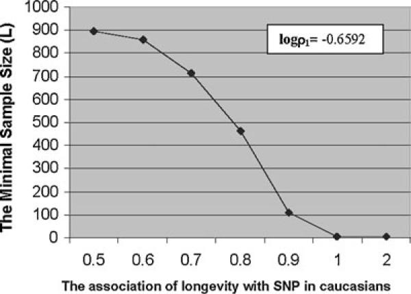
The sample size (minimal L) curve when logρ₁ (association of SNP with race in centenarians) and four marginal frequencies are fixed at those values of the 17th SNP and logρ_ca (association of SNP with longevity in Caucasians) varies from 0.5 to 1.0 with in increments of 0.1. The minimal L is obtained under the conditions: α = 0.05, 1 − β = 0.8 and the number of young controls N = 400.

To show the effects of the odds ratio ρ_ca on the sample size needed, the sample size (the minimum number of the case total) was computed using five fixed parameters [logρ₁ and four margin frequencies (p, q, r, s) from the 17th SNP and one varying parameter logρ_ca association of longevity with SNP in Caucasians]. This condition means that in the 2 × 2 × 2 probability table, the probability table for the centenarians is fixed, while the probability table for the young controls varies (consistent with the fact that the probability structure of centenarians in Georgia is not changing for this particular SNP). We have obtained the sample sizes as the logρ_ca varies from 0.5 to 1.0 in increments of 0.1 (Figure 1). The sample size necessary to detect the associations between factors of interest increases from 4 to more than 900 as the logρ_ca varies from 1.0 to 0.5. In this example logρ₁ is fixed at −0.6592. The results showed that the required sample size changes dramatically as the logρ_ca varies from a small number to a relatively large number. For the 17th SNP, an association with longevity can be detected down to about logρ_ca ≅ 0.86 from Figure 1. It indicates that the probability table of the control group plays a very important role in determining the power of the statistical test in our study when other parameters are fixed. We can also see that when the log odds ratios are close to zero, that is, the nonrandom associations are very small, a large sample size is required to detect associations.

Table 4 shows a comparison between the exact method, MCMC and asymptotic analysis for the sample size problem of 2 × 2 × 2 tables for some of the SNPs under the same conditions. For SNPs that require relatively large L values to detect the associations determined by the exact method, such as SNPs 15, 24, 26, and 27, the Ls determined by MCMC are close to the corresponding Ls required by the exact method. However, for SNPs that require relatively small L values to detect associations, such as SNPs 17, 18, and 1, the L values determined by MCMC are generally smaller than the Ls required by the exact method, and the N values are also smaller than 400. Compared to the results of the exact method and MCMC, the L values determined by the asymptotic analysis are smallest. The CPU time used by exact method is on average 10.16 [S.D. = 9.98, S.E. = 9.88/sqrt(12) = 2.60] times the corresponding time used by MCMC method depending on the SNPs considered.

Table 4.

A comparison between the exact method, the MCMC method, and the asymptotic analysis for the sample size problem of 2 × 2 × 2 tables for some SNPs when α = 0.05, 1 − β = 0.8. The first three columns represent the minimal numbers of centenarian alleles (L), and the second block of three columns represents the numbers of young control alleles (N) needed using these three methods, respectively. The last two columns are the CPU time used by the exact method and MCMC method, respectively. The exact method was implemented in parallel on a 32-node processor; the MCMC method was implemented on one node of the same 32-node processor.

	L			N			Time (hours)
SNPs	Exact	MCMC	Asympt	Exact	MCMC	Asympt	Exact	MCMC
SNPs_17	4	1	1	400	56	24	154.76	17.37
SNPs_18	16	1	1	400	45	18	79.71	17.07
SNPs_12	23	1	1	400	252	92	19.59	4.18
SNPs_l	54	1	1	400	84	34	108.64	3.95
SNPs_6	85	89	1	400	400	273	30.18	8.82
SNPs_21	100	1	1	400	330	107	23.84	1.74
SNPs_23	136	122	1	400	400	299	42.81	2.1
SNPs_15	180	201	1	400	400	157	139.32	76.15
SNPs_5	310	336	1	400	400	132	589.56	99.11
SNPs_24	406	378	1	400	400	304	127.97	4.53
SNPs_26	3312	3315	311	400	400	400	816.34	688.74
SNPs_27	4495	4515	771	400	400	400	2375.46	1660.62

4. Discussion

Many medical and biological studies involve a 2 × 2 × 2 table, and many of these studies use two independent samples, case and control. Our study provides a solution for the sample size problem for an omnibus exact test for detecting nonrandom associations in a 2 × 2 × 2 table, and does not test for individual nonrandom associations in a particular direction in the parameter space (e.g., a particular odds ratio). Our results facilitate experimental researchers optimizing their sampling method by providing a method for computing the minimum sample size needed to detect nonrandom associations in 2 × 2 × 2 tables. Solving the sample size problem is a computationally intensive process. The time in seconds to calculate the power for the test with the sample size L and N is approximately linear in L³N³. In this case, parallel computing techniques were necessary for implementation. We would also like to point out that in those cases where the nonrandom associations between the factors of interest are very small, it takes more computation time to obtain the minimum L. A comparison between the results of the exact method and those of the MCMC method showed that for SNPs that require relatively large L values to detect the associations, MCMC provides a very good approximation faster (10.14 times on average for examples considered) than our exact method as suggested by Guo and Thompson (1992) in another context. However, for SNPs that require small L values to detect the associations, the exact method is the only method to provide the correct solutions.

It should be noted that there are several forms of the exact test (Yates, 1984; Agresti, 1992) including: (i) Fisher's one-sided exact test where the larger of the two tails is not larger than α/2; (ii) Fisher's one-sided exact test where the larger of the two tails is not larger than α; and (iii) Fisher's two-sided exact test. Fu and Arnold (1992) did not find appreciable differences in the solutions for these three tests for 2 × 2 tables. It was also found that the two-sided test tended to be the most conservative with respect to sample size. For these reasons and others (Sánchez et al., 2006), solutions for the sample size problem for the 2 × 2 × 2 table have only been reported for the two-sided test against an omnibus alternative.

An interesting generalization of the sample size problem considered here is a multiple testing problem involving hundreds or even thousands of SNPs simultaneously (Zou and Zuo, 2006). In solving the sample size problem they try to control FDR or related criterion and use an asymptotic solution for the samples sizes with all of its inherent limitations. As shown under results, a sample size recommendation can be made to control FDR without resorting asymptotic solutions for the sample sizes.

References

- Agresti A. A survey of exact inference for contingency tables. Statistical Science. 1992;7:131–153. [Google Scholar]
- Agresti A, Wackerly D, Boyett JM. Exact conditional tests for cross-classifications: Approximation of attained significance levels. Psychometrika. 1979;44:75–83. [Google Scholar]
- Benjamini Y, Hochberg Y. Controlling the false discovery rate—A practical and powerful approach to multiple testing. (Series B).Journal of Royal Statistical Society. 1995;57:289–300. [Google Scholar]
- Bennett BM, Hsu P. On the power function of the exact test for the 2 × 2 contingency table. Biometrika. 1960;47:393–398. Correction 48(1961), 475. [Google Scholar]
- Besag J, Clifford P. Generalized Monte Carlo significance tests. Biometrika. 1989;76:633–642. [Google Scholar]
- Carey J. Longevity: The Biology and Demography of Life Span. Princeton University Press; Princeton and Oxford: 2003. [Google Scholar]
- Casagrande JT, Pike MC, Smith PG. An improved approximate formula for calculating sample sizes for comparing two binomial distributions. Biometrics. 1978;29:441–448. [PubMed] [Google Scholar]
- Finch CE. Longevity, Senescence, and the Genome. University of Chicago Press; Chicago: 1990. [Google Scholar]
- Fisher RA. The logic of inductive inference. (Series A).Journal of Royal Statistical Society. 1935;98:39–54. [Google Scholar]
- Fleiss JL. Statistical Methods. 2nd edition Wiley; New York: 1981. [Google Scholar]
- Franceschi C, Olivieri F, Marchegiani F, Cardelli M, Cavallone L, Capri M, Salvioli S, Valensin S, De Benedictis G, Di Iorio A, Caruso C, Paolisso G, Monti D. Genes involved in immune response/inflammation, IGF1/insulin pathway and response to oxidative stress play a major role in the genetics of human longevity: The lesson of centenarians. Mechanisms of Ageing and Development. 2005;126:351–361. doi: 10.1016/j.mad.2004.08.028. [DOI] [PubMed] [Google Scholar]
- Fu YX, Arnold J. A table of exact sample sizes for use with Fisher's exact test for 2 × 2 tables. Biometrics. 1992;48:1103–1112. [Google Scholar]
- Gail M, Gart J. The determination of sample sizes for use with the exact conditional test in 2 × 2 comparative trials. Biometrics. 1973;29:441–448. [PubMed] [Google Scholar]
- Guo SW, Thompson EA. Performing the exact test of Hardy-Weinberg proportion for multiple alleles. Biometrics. 1992;48:361–372. [PubMed] [Google Scholar]
- Hagmann M. A good SNP may be hard to find. Science. 1999;285:21–22. doi: 10.1126/science.285.5424.21a. [DOI] [PubMed] [Google Scholar]
- Harter HL, Owen DB. Selected Tables in Mathematical Statistics. Volume 1. Markham Publishing Company; Chicago, Illinois: 1970. [Google Scholar]
- Hasemen JK. Exact sample sizes for use with the Fisher-Irwin test for 2×2 tables. Biometrics. 1978;34:106–109. [Google Scholar]
- Haynam GE, Govindarajulu Z, Leone FC. Tables of the cumulative noncentral chi-square distribution. In: Harter HL, Owens DB, editors. Selected Tables in Mathematical Statistics. Volume 1. Markham Publishing; Chicago, Illinois: 1970. [Google Scholar]
- Karasik D, Demissie S, Cupples LA, Kiel DP. Disentangling the genetic determinants of human aging: Biological age as an alternative to the use of survival measures. (Series A: Biological Sciences and Medical Sciences).The Journals of Gerontology. 2005;60:574–587. doi: 10.1093/gerona/60.5.574. [DOI] [PMC free article] [PubMed] [Google Scholar]
- Kervinen K, Savolainen MJ, Salokannel J, Hynninen A, Heikkinen J, Ehnholm C, Koistinen MJ, Kesaniemi YA. Apolipoprotein E and B polymorphisms—Longevity factors assessed in nonagenarians. Atherosclerosis. 1994;105:89–95. doi: 10.1016/0021-9150(94)90011-6. [DOI] [PubMed] [Google Scholar]
- Kreiner S. Analysis of multi-dimensional contingency tables by exact conditional tests: Techniques and strategies. Scandinavian Journal of Statistics. 1987;14:97–112. [Google Scholar]
- Lander ES, Schork NJ. Genetic dissection of complex traits. Science. 1994;265:2037–2048. doi: 10.1126/science.8091226. [DOI] [PubMed] [Google Scholar]
- Louhija J, Miettinen HE, Kontula K, Tikkanen MJ, Miettinen TA, Tilvis RS. Aging and genetic variation of plasma apolipoproteins: Relative loss of apolipoprotein E4 phenotype in centenarians. Atherosclerosis and Thrombosis. 1994;14:1084–1089. doi: 10.1161/01.atv.14.7.1084. [DOI] [PubMed] [Google Scholar]
- Mielke PW, Berry KJ. Cumulant methods for analysing independence of r-way contingency tables and goodness-of-fit frequency data. Biometrika. 1988;75:790–793. [Google Scholar]
- Poon LW, Jazwinski SM, Green RC, et al. Contributors of longevity and adaptation: Findings and new directions from the Georgia Centenarian Study. In: Perls T, editor. Exceptional Longevity. Johns Hopkins University Press; Baltimore, Maryland: 2006. [Google Scholar]
- Proust J, Moulias R, Fumeron F, Bekkhoucha F, Busson M, Schmid M, Hors J. HLA and longevity. Tissue Antigens. 1982;19:168–173. doi: 10.1111/j.1399-0039.1982.tb01436.x. [DOI] [PubMed] [Google Scholar]
- Roberts GO, Gelman A, Gilks WR. Weak convergence and optimal scaling of random walk Metropolis algorithms. Annals of Applied Probability. 1997;7:110–120. [Google Scholar]
- Sánchez M, Basten C, Ferrenberg A, Asmussen A, Arnold J. Exact sample sizes needed to detect dependence in 2 × 3 tables. Theoretical Population Biology. 2006;69:111–120. doi: 10.1016/j.tpb.2005.11.001. [DOI] [PubMed] [Google Scholar]
- Schachter F, Faure-Delanef L, Guenot F, Rouger H, Froguel P, Lesueur-Ginot L, Cohen D. Genetic associations with human longevity at the APOE and ACE loci. Nature Genetics. 1994;6:29–32. doi: 10.1038/ng0194-29. [DOI] [PubMed] [Google Scholar]
- Smith PWF, Forster JJ, McDonald JW. Monte Carlo exact tests for square contingency tables. (Series A).Journal of the Royal Statistical Society. 1996;159:309–321. [PubMed] [Google Scholar]
- Snir MF, Otto S, Shuss-Lederman S, Walker D, Dongarra J. MPI the Complete Reference. MIT Press; Cambridge, Massachusetts: 1998. [Google Scholar]
- Storey JD. A direct approach to false discovery rates. (Series B).Journal of the Royal Statistical Society. 2002;64:479–498. [Google Scholar]
- Takata H, Suzuki M, Ishii T, Sekiguchi S, Iri H. Influence of major histocompatibility complex region genes on human longevity among Okinawan-Japanese centenarians and nonagenarians. Lancet. 1987;II:824–826. doi: 10.1016/s0140-6736(87)91015-4. [DOI] [PubMed] [Google Scholar]
- The International HapMap Consortium A haplotype map of the human genome. Nature. 2005;437:1299–1320. doi: 10.1038/nature04226. [DOI] [PMC free article] [PubMed] [Google Scholar]
- Verhoeven KJF, Simonsen KL, McIntyre LM. Implementing false discovery rate: Increasing your power. Oikos. 2005;108:643–647. [Google Scholar]
- Yates F. Test of significance for 2 × 2 contingency tables. (Series A).Journal of the Royal Statistical Society. 1984;147:426–463. [Google Scholar]
- Zelterman D, Chan ISF, Mielke PW. Exact tests of significance in higher dimensional tables. American Statistician. 1995;49:357–361. [Google Scholar]
- Zou G, Zuo Y. On the sample size requirement in genetic association tests when the proportion of false positives is controlled. Genetics. 2006;172:687–691. doi: 10.1534/genetics.105.049536. [DOI] [PMC free article] [PubMed] [Google Scholar]