Improved Fitting of Solution X-ray Scattering Data to Macromolecular Structures and Structural Ensembles by Explicit Water Modeling

Abstract

A new procedure, AXES, is introduced for fitting small-angle X-ray scattering (SAXS) data to macromolecular structures and ensembles of structures. By using explicit water models to account for the effect of solvent, and by restricting the adjustable fitting parameters to those that dominate experimental uncertainties, including sample/buffer rescaling, detector dark current, and, within a narrow range, hydration layer density, superior fits between experimental high resolution structures and SAXS data are obtained. AXES results are found to be more discriminating than standard Crysol fitting of SAXS data when evaluating poorly or incorrectly modeled protein structures. AXES results for ensembles of structures previously generated for ubiquitin show improved fits over fitting of the individual members of these ensembles, indicating these ensembles capture the dynamic behavior of proteins in solution.

Solution small-angle X-ray scattering (SAXS) data contain valuable information on the macromolecular size and shape and are increasingly used in biomolecular structure studies, not only as a stand alone tool but as a complement to NMR and X-ray crystallography.¹⁻⁴ Recent methods permit direct refinement against X-ray scattering data in combination with other experimental restraints, taking advantage of the sensitivity of these data to the molecular shape.⁵⁻⁸ In particular, the long-range translational information encoded in SAXS data is proving to be a valuable complement to global orientational restraints contained in NMR residual dipolar couplings. As these solution data reflect the composition of the entire structural ensemble, they are also particularly useful in the investigation of flexible and intrinsically disordered systems, which often challenge a detailed structural characterization by X-ray crystallography and conventional NMR.(9)

The utility of SAXS data in structural studies critically hinges on the ability to accurately predict such data from all-atom structural models. Important progress in this area has been made over the past two decades, leading to an established formalism for such calculations, culminating in the Crysol software package,(10) the de facto standard for such calculations. Crysol models solution scattering data from a uniform orientational average:

where F_mol, F_disp, and δρF_surf stand for the complex scattering amplitudes of the macromolecule, the displaced solvent, and the increased density (by δρ) of the surface water layer. The scattering vector is defined as q = 4π sin θ/λ, where 2θ is the scattering angle and λ is the incident radiation wavelength.

Other methods have been formulated to improve on the treatment of orientational averaging and solvent representation.¹¹⁻¹⁴ However, Crysol’s speed, simplicity, and often superior ability to obtain a very good fit of the experimental scattering data to the atomic coordinates make its use very attractive. Several adjustable parameters are used by Crysol when calculating predicted data that best match the experimental curve. Next to the adjustable overall scaling factor between the measured and fitted data, these include the effective atomic radii multiplier which scales the solvent volume displaced by each atom, the electron density contrast of the surface solvent layer, and the total displaced solvent volume, in practice equivalent to the variation of the electron density of the displaced solvent relative to bulk water. The necessity for introducing these parameters as variables rather than constants that are kept fixed for all proteins or nucleic acids is not immediately obvious from first principles but becomes clear when investigating the reproducibility of experimental scattering data collected for distinct samples of the same macromolecule on different instruments. Such comparisons often indicate that the characteristic features of the measured scattering curves are well conserved, but in particular the scattered intensity at larger angles (“higher-q features”) varies relative to the extrapolated intensity at zero angle, I(0). Crysol’s adjustable parameters are very effective at absorbing this variability as they can adjust the level of the higher-q features of the predicted data relative to the low-q intensities.

Here, we reformulate the approach to fitting SAXS data by explicitly taking into account the sources of experimental data variability. For this purpose, the measured scattering intensity difference is written as

where the variable sample/buffer rescaling factor α ≈ 1 accounts for the uncertainty in the measurements of transmitted and incident intensities and the concentration-based uncertainty at which the solute volume fraction in the sample is known. The second variable, c, accounts for variability of the detector’s dark current and effects such as X-ray fluorescence. Uncertainties in α and c appear responsible for much of the systematic difference between repeated experimental data sets. In our analysis, we model the scattering intensity predicted from the atomic coordinates as

Here, the Ω average is taken over a discrete pseudouniform set of molecular frame orientations relative to the incident beam; the “solv” average is taken over the displaced and surface water sets; and “ens” denotes an average over the ensemble of macromolecular structures, when available.

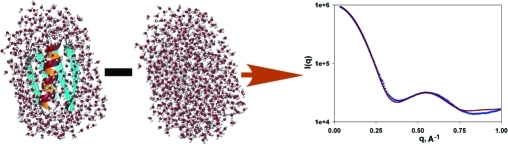
In our approach, the scattering amplitudes of the surface and displaced solvent are calculated by summations over explicit individual water molecules, as detailed in the Supporting Information (SI). Explicit and realistic representation of the solvent is particularly useful for molecular shapes that strongly deviate from being globular, including rods, toroids, dumbbells, random coils, and other highly anisometric shapes. A second advantage of this approach is its natural ability to predict the scattering intensities for an arbitrarily dynamic ensemble with the same ease as that for a single static structure. So, our approach uses the same number of adjustable parameters as Crysol but replaces the atomic radii multiplier and total excluded volume, which are applied to the structure-predicted data, by the solvent/buffer rescaling factor and the constant offset, applied to the measured data.

A measure of the discrepancy, D, between the predicted and measured scattering data is formulated as

Here, A is the overall scaling parameter, σ_expt are the experimental uncertainties for each individual data point, R(α) is a regularizer which keeps the fitted α parameter close to the target value for the concentration-based volume fraction of the displaced solvent, α_o, and σ_α ≈ 10⁻² denotes the uncertainty of this parameter. Fitting of the SAXS data is carried out by our webserver program AXES (Analysis of X-ray scattering data for Ensemble Structures; http://spin.niddk.nih.gov/bax/nmrserver/), using a Powell minimization of the penalty function against the adjustable parameters for both experimental (α, c) and predicted (A, δρ) data.

Superior SAXS data fit quality is illustrated for a set of small well-studied proteins for which high-resolution structures were available from X-ray crystallography and solution NMR.¹⁵⁻¹⁸ SAXS data for hen egg white lysozyme, cytochrome c, the B3 domain of protein G (GB3), and ubiquitin were acquired at the BIOCAT and BESSRC beamlines at the Advanced Photon Source synchrotron and fitted up to q values of ∼1 Å⁻¹. We limit the fitting of our SAXS data to q < 1 Å⁻¹ as, on one hand, scattering data above 1 Å⁻¹ become increasingly similar for different proteins(19) and, on the other, the ability to accurately model such data is hampered by coordinate uncertainties, macromolecular dynamics, inhomogeneity of the surface solvent distribution, the effects of inelastic (Compton) scattering, and the accuracy of the commonly used neutral-atom form factors. Improvements in the data fit quality (Figure 1; Table 1; SI) indicate that the AXES program yields χ decreases of 10−50% over Crysol analysis, also for larger systems. When normalizing the fitting error to the very low statistical error associated with the high photon counts obtained for our synchrotron measurements, the residual error in the fit becomes dominated by the presence of small systematic errors resulting from fluctuations in temperature, beam position, transmission, and beam path length, as well as the imperfections in the data modeling noted above, resulting in χ >1. Using the same input data and number of adjustable fitting parameters, lower χ values obtained with AXES fitting compared to CRYSOL reflect smaller imperfections in the data modeling. As currently implemented, AXES is more than an order of magnitude slower than Crysol due to the need to average the scattering amplitudes involving the displaced and surface solvent over ca. 20 independent configurations. Applications of AXES-like methodology for direct inclusion in structure refinement programs^5−7,20 will require a significant speedup; several possible avenues for such speedup are currently under development.

Figure 1.

Comparison of experimental (black) with predicted (red) SAXS data generated by (A) standard Crysol and (B) AXES fitting. From top to bottom, data sets correspond to GB3, cytochrome C, lysozyme, and ubiquitin (PDB entries 1IGD, 1CRC, 193L, and 1D3Z). Data sets are arbitrarily offset vertically for visual purposes.

Table 1. Fitting Statistics (χ Values) Obtained with Crysol and AXES for Four Proteins.

	Lysozyme	Cytochrome C	GB3	Ubiquitin
Crysol	1.19	1.93	4.70	3.60
AXES	0.98	0.90	1.76	3.05

More important than the drop in χ statistics afforded by AXES is the question whether the program can discriminate well against poor models on the basis of SAXS data. For this purpose, we fit the experimental GB3 data to 2000 models generated de novo by the program Rosetta.(21) All Rosetta generated structures by their very nature are quite compact and have comparable radii of gyration (R_g = 11.1 ± 0.4 Å), but many have high Rosetta energies indicative of incorrect folds, deviating by 5 Å or more from the X-ray reference structure (PDB entry 1IGD).(15) Fits of the SAXS data by the standard approach in many cases yields χ values that are much lower, by up to 70%, for poor models (i.e., high rmsd to 1IGD) than those for the X-ray reference structure (Figure 2A), indicative of overfitting. In contrast, AXES does not yield significantly better fits for any of the poor Rosetta models (Figure 2B). At the same time, the AXES results illustrate that for a subset of the poor structures SAXS data alone cannot discriminate these from the reference structure. When restricting ourselves to models that all have the correct fold, as generated by chemical-shift-guided CS-Rosetta(22) (blue dots in Figure 2), AXES correctly assigns higher relative χ values (1.6 ± 0.5) to the CS-Rosetta models than to the experimental structure, whereas the inverse applies for the standard SAXS fitting procedure (χ = 0.93 ± 0.18; Figure 2A).

Figure 2.

Normalized χ values when fitting 2000 GB3 models, generated by Rosetta (red) or CS-Rosetta (blue) modeling, to experimental SAXS data using (A) standard Crysol and (B) AXES fits. The horizontal axis corresponds to the backbone C^α rmsd between the model and the X-ray structure (PDB entry 1IGD); χ values are normalized relative to the χ_1IGD value obtained when fitting the X-ray structure (horizontal black line).

An important feature of AXES is its ability to directly fit structural ensembles. Remarkably, fits to the previously extensively studied dynamic ensemble representations of ubiquitin^23,24 yield lower χ values when fitting these entire ensembles simultaneously, than when fitting each member of the ensemble separately, followed by averaging of these χ values (χ_ensemble = 5.06 and 4.98 for PDB entries 1XQQ(23) and 2K39,(24) respectively, vs ⟨χ⟩ = 5.36 for 1XQQ and ⟨χ⟩ = 6.01 for 2K39; SI), despite far fewer adjustable parameters in the fitting procedure (4 for the ensemble fit; N*4 for an N-member ensemble). Even though the AXES fit to the static, lowest energy NMR structure (1D3Z;(25) χ = 3.05) suggests that this model is a better representation of the average ubiquitin structure in solution, the fact that fits to the entire 1XQQ and 2K39 ensembles are better than those to their individual members indicates that these ensembles correctly capture dynamic processes in the protein. The ability to evaluate such ensemble fits is becoming increasingly important as experimental structural biology shifts from an average-model view of macromolecular structure to more realistic multistate representations.

Supporting Information Available

Details of the calculation of the predicted scattering data; procedures for sample preparation; experimental data collection; processing and analysis; results for GB3, ubiquitin, malate synthase G, and maltose binding protein. This material is available free of charge via the Internet at http://pubs.acs.org.

Funding Statement

National Institutes of Health, United States

References

- Svergun D. I.; Koch M. H. J. Rep. Prog. Phys. 2003, 66, 1735–1782. [Google Scholar]
- Putnam C. D.; Hammel M.; Hura G. L.; Tainer J. A. Q. Rev. Biophys. 2007, 40, 191–285. [DOI] [PubMed] [Google Scholar]
- Columbus L.; Lipfert J.; Jambunathan K.; Fox D. A.; Sim A. Y. L.; Doniach S.; Lesley S. A. J. Am. Chem. Soc. 2009, 131, 7320–7326. [DOI] [PMC free article] [PubMed] [Google Scholar]
- Bertini I.; Calderone V.; Fragai M.; Jaiswal R.; Luchinat C.; Melikian M.; Mylonas E.; Svergun D. I. J. Am. Chem. Soc. 2008, 130, 7011–7021. [DOI] [PubMed] [Google Scholar]
- Grishaev A.; Wu J.; Trewhella J.; Bax A. J. Am. Chem. Soc. 2005, 127, 16621–16628. [DOI] [PubMed] [Google Scholar]
- Schwieters C. D.; Clore G. M. Biochemistry 2007, 46, 1152–1166. [DOI] [PubMed] [Google Scholar]
- Zuo X. B.; Wang J. B.; Foster T. R.; Schwieters C. D.; Tiede D. M.; Butcher S. E.; Wang Y. X. J. Am. Chem. Soc. 2008, 130, 3292–3293. [DOI] [PubMed] [Google Scholar]
- Grishaev A.; Tugarinov V.; Kay L. E.; Trewhella J.; Bax A. J. Biomol. NMR 2008, 40, 95–106. [DOI] [PubMed] [Google Scholar]
- Bernado P.; Mylonas E.; Petoukhov M. V.; Blackledge M.; Svergun D. I. J. Am. Chem. Soc. 2007, 129, 5656–5664. [DOI] [PubMed] [Google Scholar]
- Svergun D.; Barberato C.; Koch M. H. J. J. Appl. Crystallogr. 1995, 28, 768–773. [Google Scholar]
- Zuo X. B.; Tiede D. M. J. Am. Chem. Soc. 2005, 127, 16–17. [DOI] [PubMed] [Google Scholar]
- Yang S. C.; Park S.; Makowski L.; Roux B. Biophys. J. 2009, 96, 4449–4463. [DOI] [PMC free article] [PubMed] [Google Scholar]
- Merzel F.; Smith J. C. Proc. Natl. Acad. Sci. U.S.A. 2002, 99, 5378–5383. [DOI] [PMC free article] [PubMed] [Google Scholar]
- Park S.; Bardhan J. P.; Roux B.; Makowski L. J. Chem. Phys. 2009, 130, 134114. [DOI] [PMC free article] [PubMed] [Google Scholar]
- Derrick J. P.; Wigley D. B. J. Mol. Biol. 1994, 243, 906–918. [DOI] [PubMed] [Google Scholar]
- Ulmer T. S.; Ramirez B. E.; Delaglio F.; Bax A. J. Am. Chem. Soc. 2003, 125, 9179–9191. [DOI] [PubMed] [Google Scholar]
- Vaney M. C.; Maignan S.; RiesKautt M.; Ducruix A. Acta Crystallogr., Sect. D: Biol. Crystallogr. 1996, 52, 505–517. [DOI] [PubMed] [Google Scholar]
- Sanishvili R.; Volz K. W.; Westbrook E. M.; Margoliash E. Structure 1995, 3, 707–716. [DOI] [PubMed] [Google Scholar]
- Svergun D. I.; Petoukhov M. V.; Koch M. H. J. Biophys. J. 2001, 80, 2946–2953. [DOI] [PMC free article] [PubMed] [Google Scholar]
- Grishaev A.; Ying J.; Canny M. D.; Pardi A.; Bax A. J. Biomol. NMR 2008, 42, 99–109. [DOI] [PMC free article] [PubMed] [Google Scholar]
- Bradley P.; Misura K. M. S.; Baker D. Science 2005, 309, 1868–1871. [DOI] [PubMed] [Google Scholar]
- Shen Y.; Lange O.; Delaglio F.; Rossi P.; Aramini J. M.; Liu G. H.; Eletsky A.; Wu Y. B.; Singarapu K. K.; Lemak A.; Ignatchenko A.; Arrowsmith C. H.; Szyperski T.; Montelione G. T.; Baker D.; Bax A. Proc. Natl. Acad. Sci. U.S.A. 2008, 105, 4685–4690. [DOI] [PMC free article] [PubMed] [Google Scholar]
- Lindorff-Larsen K.; Best R. B.; DePristo M. A.; Dobson C. M.; Vendruscolo M. Nature 2005, 433, 128–132. [DOI] [PubMed] [Google Scholar]
- Lange O. F.; Lakomek N. A.; Fares C.; Schroder G. F.; Walter K. F. A.; Becker S.; Meiler J.; Grubmuller H.; Griesinger C.; de Groot B. L. Science 2008, 320, 1471–1475. [DOI] [PubMed] [Google Scholar]
- Cornilescu G.; Marquardt J. L.; Ottiger M.; Bax A. J. Am. Chem. Soc. 1998, 120, 6836–6837. [Google Scholar]
Associated Data
This section collects any data citations, data availability statements, or supplementary materials included in this article.