A Scale-Free Structure Prior for Graphical Models with Applications in Functional Genomics

Abstract

The problem of reconstructing large-scale, gene regulatory networks from gene expression data has garnered considerable attention in bioinformatics over the past decade with the graphical modeling paradigm having emerged as a popular framework for inference. Analysis in a full Bayesian setting is contingent upon the assignment of a so-called structure prior—a probability distribution on networks, encoding a priori biological knowledge either in the form of supplemental data or high-level topological features. A key topological consideration is that a wide range of cellular networks are approximately scale-free, meaning that the fraction, , of nodes in a network with degree is roughly described by a power-law with exponent between and . The standard practice, however, is to utilize a random structure prior, which favors networks with binomially distributed degree distributions. In this paper, we introduce a scale-free structure prior for graphical models based on the formula for the probability of a network under a simple scale-free network model. Unlike the random structure prior, its scale-free counterpart requires a node labeling as a parameter. In order to use this prior for large-scale network inference, we design a novel Metropolis-Hastings sampler for graphical models that includes a node labeling as a state space variable. In a simulation study, we demonstrate that the scale-free structure prior outperforms the random structure prior at recovering scale-free networks while at the same time retains the ability to recover random networks. We then estimate a gene association network from gene expression data taken from a breast cancer tumor study, showing that scale-free structure prior recovers hubs, including the previously unknown hub SLC39A6, which is a zinc transporter that has been implicated with the spread of breast cancer to the lymph nodes. Our analysis of the breast cancer expression data underscores the value of the scale-free structure prior as an instrument to aid in the identification of candidate hub genes with the potential to direct the hypotheses of molecular biologists, and thus drive future experiments.

Introduction

Gene Regulatory Networks and Gene Expression Data

Knowledge of the interactions among genes and gene products that occur within a cell is vital for understanding cellular behavior. These activities are largely a consequence of gene expression, the process whereby genes transcribe signature mRNA molecules that are translated into gene products of numerous kinds and functions. As it happens, genes do not express independently of one another; instead, their activities are coordinated in a complex system of control in which distinguished genes, called transcriptions factors, regulate the expression of other genes via their gene product proxies.

An undirected network is a mathematical object consisting of a set of nodes and a set of unordered pairs of nodes called undirected edges. It differs from a directed network, which is also denoted by , in that the latter is defined in terms of ordered pairs of nodes known as directed edges. Applying these straightforward abstractions to cellular processes has gained currency throughout the biosciences, so much so that a network mind-set has become a necessary precondition for thinking about systems of gene regulatory interactions. For the purposes of this paper, a gene regulatory network is a directed network in which genes are identified with nodes and regulatory interactions with directed edges. From a purely statistical standpoint, it is best to regard a gene regulatory network as a convenient depiction of the true regulatory interactions of a system that, in reality, must be estimated from data.

Indeed, the network approach toward understanding gene regulatory systems only came to prominence in response to the advent of DNA microarray technology, which makes the profiling of mRNA expression levels for individual genes possible on a genome-wide scale. A typical experiment consists of a library of expression profiles, each one a snapshot of the expression levels for genes under a different experimental condition. The raw expression profile data is preprocessed and then arranged by row in an data matrix, . In practice, not only is gene expression data notoriously noisy [1], but to make matters worse the number of samples is typically at least an order of magnitude smaller than the number of genes, that is, (the “small , large ” problem), making the inference of regulatory interactions a challenging statistical problem [2].

There is now an extensive repertoire of algorithms available for the analysis of gene expression data, the majority of which are based on Boolean networks, differential equations, and graphical models [3]. Some approaches produce estimated gene regulatory networks that are directed networks, while others do not. In this paper, we work primarily with a variety of undirected graphical model known as gene association networks (GANs), in which undirected edges, called gene associations, correspond to certain statistical dependencies that are inferred from gene expression data. Therefore, in an effort to simplify the terminology, the terms “network” and “edge” will be used hereafter to mean undirected network and undirected edge, respectively. Although we will occasionally use the term “network” in a colloquial sense, such as in “network mind-set” or “network approach.” At any rate, the meaning should be clear from context.

Graphical Models

Graphical models [4], [5], [6] are a suite of probabilistic models, widely used for estimating large-scale gene regulatory networks from gene expression data [7]. In this framework, genes are identified with the random variables of a multivariate distribution with covariance matrix , and each row of is taken as a random sample from . The conditional independence structure of defines a network with the random variables as nodes and conditional dependencies latent between the random variables as directed or undirected edges; a diversity of models arise from the extent to which the dependencies are resolved [8].

Relevance networks comprise the simplest class of graphical model with absent edges corresponding to marginal independencies between the components of . These networks have long been used in the analysis of genetic data [9]. But in terms of identifying regulatory interactions, relevance networks are bound to be misleading because marginal independence alone cannot discriminate among direct and indirect dependencies.

GANs provide a better alternative, circumventing this drawback by appealing to conditional independence as a criterion for edge exclusion. Gaussian graphical models (GGMs) are the gold standard. In a GGM, a pair of nodes do not share an edge when their underlying random variables from are conditionally independent given all of the remaining random variables. However, GGMs too are not without disadvantages, as their estimation can be computationally intensive in a “small , large ” setting [10]. A class of GANs, bridging the gap between relevance networks and GGMs, has been advanced with this consideration in mind where absent edges are identified with lower order conditional independencies [11], [12], [13].

Lastly, Bayesian networks are a variety of graphical model founded on a more refined notion of conditional independence, conferring directionality to the edges; they are also well-established as a methodology for estimating gene regulatory networks [14].

The Structure Prior

Inference within the graphical modeling paradigm amounts to an often painstaking exercise in covariance estimation and model selection. We defer a discussion on the problem of covariance estimation to the Methods section. That is because our interest pertains to model selection, which in a Bayesian setting is accomplished by sampling from the posterior distribution

(1)

over the appropriate space of networks using either heuristic searches or else Markov chain Monte Carlo (MCMC). The term is the likelihood and the structure prior, that is, a prior assigning a probability to each possible network.

The role of the structure prior is to direct inference toward graphical models consistent with biological prior knowledge, which may come in the form of a priori topological considerations or from a posteriori sources apart from the dataset. As far as the latter is concerned, previous research has concentrated on Bayesian networks [15], [16], [17], [18]. On the other hand, biologically-motivated topological assumptions are a consistent feature of graphical models tailored for genetic data. Heuristic search strategies often include implicit assumptions concerning network sparsity [19], [20], [21], [22]. In instances in which the structure prior is given explicit specification, standard practices include using a uniform prior capped at a small number of potential regulators per gene [23], or assigning it as a sparse random network [24], [25].

Random and Scale-Free Networks

The theory of random networks was given its first systematic expression by Erdös and Rényi [26], [27]. According to the theory, a -node random network is defined by an eponymous, generating algorithm — the Erdös-Rényi (ER) model — that works by connecting each pair of nodes in an initially empty network independently with probability . This simple procedure gives rise to a probability distribution over the space of -node networks, which is used to define the so-called random structure prior, . The degree distribution — the probability that a given node is connected to other nodes — of a random network is binomially distributed according to where the degree, , of a node denotes the number of edges incident upon it. It follows, therefore, that degree in a random network has a strong central tendency, implying that the average degree of a random network is representative of the degree of a typical node.

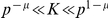
Empirical studies, however, have firmly established that a wide variety of large-scale networks in nature, society, and technology exhibit heavy-tailed degree distributions that cannot be accounted for by random network theory [28], [29], [30]. This property is often approximately described by a power-law degree distribution, , over a large range of with exponent typically between and . A network that follows a power-law is called scale-free. It gets this name because the functional form of is retained under a scaling of the argument by a constant factor : . The scale-free property is thought to be a key organizational feature of cellular networks [31], and analyses suggest such an architecture for the gene regulatory networks of the model organisms S. cerevisiae [32] and C. elegans [33].

Introducing a Scale-Free Structure Prior

Proposing a structure prior which incorporates the scale-free property is the topic of this paper. We define the scale-free structure prior, , according to the probability of a network under a simple, scale-free network model. As for the underlying network model itself, a multitude of candidates have been proposed in the literature [34]. They fall into two broad categories: 1) growing models, where a network is generated via the successive addition of nodes and edges to a small seed network, and 2) non-growing models, where to a fixed number of nodes, pairs of nodes are chosen randomly and connected by edges.

The growing model approach employs a handful of simple universal mechanisms, thought to underpin disparate natural phenomena, to drive the stochastic evolution of networks toward power-laws. Preferential attachment is, perhaps, the best known mechanism. The idea works something like this: the probability of attaching an edge from a newly added node to a node already in the system is roughly proportional to the degree of the old node. The Bárabasi-Albert (BA) model [35] is the latter-day progenitor of a wide variety of preferential attachment models. The BA model generates a network via the successive addition of nodes and edges to a small seed network. At each step, a node is added to the system with a fixed number of emanating edges, which are subsequently preferential attached to the existing nodes. The resulting network follows a power-law with on average.

Preferential attachment is not considered to be the main driving force behind genome evolution; instead, gene (node) duplication and point mutations (edge dynamics) play the dominant role in shaping of gene regulatory networks [36]. The duplication model as formulated by [37] is such a network model, which in an analysis by [38] is suggested to approximately follow a power-law.

By contrast, in the non-growing approach, each node is assigned a fixed weight with the probability of a particular network depending on those weights. The ER model is an example of a non-growing model with uniform weights. Another non-growing model is the static model [39], which is a generalization of the ER model that has been shown to follow a power-law with tunable to any value greater than , depending on the specification of the model parameters; see Methods for details. We use the static model to define . Indeed, this model is an appealing candidate for the purpose as the probability of a network is easy to compute compared with growing models of similar complexity. Moreover, the static model actually includes the ER model as a limiting case.

A New Metropolis-Hastings Sampler for Networks

We implement an MCMC algorithm with for GGMs adapted from [25], although it is important to point out that our methodology applies to graphical models in general. Reworking the algorithm is not simply a matter of plugging in a formula for because it depends furthermore on a labeling of the nodes of . Confronted with this complication, we design a novel Metropolis-Hastings sampler that solves the problem by including a node labeling, , which is defined in the Methods section, as a variable in the state space, thereby allowing it to be estimated.

Summary of Contributions

In this paper, we advance a scale-free structure prior, , for graphical models defined by the formula for the probability of a network under the static model. Our objective is to compare the performance of this prior with the commonly used random structure prior, , in the arena of simulation as well as with a real data example. We choose GGMs for this purpose, modifying the MCMC algorithm of [25] to include . As mentioned above, one challenge of implementing is that, unlike with , it requires a labeling of the nodes of . We address this issue by introducing a Metropolis-Hastings sampler that includes the node labeling as a variable in the state space.

In a simulation study, we generate networks with given degree distributions together with Gaussian data in accordance with their implied conditional independence structures. As a case study we show that and are equally effective at recovering a random network, but that is comparatively ineffective at recovering a scale-free network. In the full simulation study, we confirm that the aforementioned result holds, illustrating our main conclusion: recovers random networks on an equal footing with the , yet surpasses it in recovering scale-free networks. Finally, we illustrate our methodology by analyzing a real gene expression dataset taken from a breast cancer tumor study by [40], showing that in contrast with the random structure prior, the scale-free structure prior recovers hubs, including the estrogen regulator FOXA1 and the zinc transporter SLC39A6, which was previously unrecognized as a hub.

Methods

Network Notation

The terms “network” and “graph” are used synonymously throughout this paper. An undirected network is a mathematical object defined by a set of nodes together with a set of undirected edges consisting of unordered pairs taken from , provided that . The set of all -node, undirected networks is denoted by . A directed network is defined in an analogous manner, save that the elements of are ordered pairs called directed edges; is called the parent and the child.

It should be understood that a network refers to an undirected network, and likewise an edge is to be understood to mean an undirected edge. However, the following definitions are applicable to both undirected and directed networks. An empty network has no edges, that is , while, in a complete network is defined as the cross product . A subnetwork of is a network whose node set is a subset of , and whose edges are a subset of restricted to . The subnetwork of induced by a given subset of nodes is the subnetwork containing all edges from that connect nodes in . Two nodes are said to be neighbors when they are connected by an edge. And, a network is itself connected when every pair of nodes is connected by a sequence of neighbors. Finally, a node labeling is a permutation of the integers , applied to the nodes of so that each is represented by the integer ; see Figure 1. This node labeling is used later for defining the structure prior.

Figure 1. An example of a node labeling.

A node labeling, , of the nodes of a network with nodes so that, for instance, and .

Gaussian Graphical Models

In this section we sketch out the theory of GGMs essential to this paper. A detailed overview of the GGM estimation procedures outlined here is described in [25], while [8] is a good starting point for understanding the niche they occupy in the larger context of graphical models.

Let 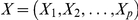be a -dimensional Gaussian random vector with zero-mean and positive definite covariance matrix, . Two random variables and are not conditionally independent given the remaining variables in if, and only if, there is a corresponding nonzero entry in the precision matrix, [41]. The conditional independence structure of can be represented by a network, , where is the value at node and there is an edge between and when and are not conditionally independent. A GGM for is the family of -dimensional Gaussian distributions from , constrained by the structure of .

Fitting a GGM to a given dataset — a task known as covariance selection — amounts to identifying zeros in the estimated precision matrix. In the classical setting when , ensuring that is positive definite, this is typically accomplished by inverting the estimated covariance matrix and then applying statistical tests to identify any entries significantly different from zero [4]. With genomic data, however, “small , large ” is the norm and, consequently, will not generally be invertible.

This problem can be addressed in one of two ways. One way calls for restricting inference to pairwise independencies conditioned on fewer than all remaining random variables. A relevance network, for example, is constructed by estimating the pairwise correlations between all random variables, connecting any pair with correlation exceeding a specified cutoff value [9]. A related approach goes one step beyond a relevance network by estimating a GAN based on not only marginal but also first-order conditional independencies [11].

A more ambitious approach is to compute satisfactory small sample estimates for and using Bayesian methods. Empirical Bayesian solutions are exemplified by shrinkage estimates [21] and sparsity encouraging lasso regression estimates [22]. Meanwhile, the full Bayesian scheme of [42] works by marginalizing over to compute the likelihood term in (1), using a prior that constrains elements of the precision matrix to zero depending on :

(2)

The term is multivariate Gaussian, while the prior is hyper-inverse Wishart with hyperparameters , a positive definite dispersion matrix, and , a degrees of freedom parameter. Jones et. al [25] advise a small value for as a reflection of ignorance, and take as the diagonal matrix , which assumes that the underlying Gaussian variables have common variance. A consequence of this assignment is that can be used to specify by making use of the fact that the marginal prior mode for each variance term is .

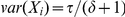GGM theory comes equipped with powerful techniques for computing the likelihood function when the underlying network is decomposable. Roughly speaking, a decomposable network can be broken down into distinguished subsets of nodes called maximal cliques. A clique is a subset of nodes whose induced subgraph is complete, and is called maximal when it is not contained within a larger complete subgraph. Computing the likelihood for a subset of corresponding to a maximal clique is particularly tractable because the density is just an unrestricted multivariate Gaussian. Hence, when a network is decomposable, the evaluation of the likelihood term in (1) reduces to the computation of many likelihoods of smaller dimension [43]. We will return to these issues in the section on our MCMC implementation.

The Static Model

A network model is a stochastic algorithm for generating networks that may depend on a vector of parameters, 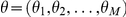. Associated with any model is a probability distribution, assigning a probability to each , where is a node labeling of .

The static network model [39] works by first assigning a weight 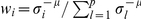to each node where , the Zipf exponent, is a tunable parameter in . To generate a network, , the following step is repeated () times: select nodes and with probabilities and and connect them with an edge, unless or and are already connected, in which case no edge is added to the network. The overall model parameter is .

In order to work out the functional form of the degree distribution, it is enough to notice that, on average, each node acquires edges in proportion to its weight. Supposing for a moment that denotes the degree of node , we may write this as . The probability distribution over the 's is known as Zipf's law, and it has been shown to be equivalent to a power-law degree distribution with [44]. It follows that the static model generates networks that follow a power-law with depending on the choice of . A rigorous derivation of the power-law appears in a comprehensive analysis of the static model by Lee et al. [45]. In the case when , the exponent, , lies between and , which is the most interesting range of values from the point of view of scale-free architecture. In contrast, for values of , which corresponds to , the tail of is less pronounced. In the limit of , or equivalently , each weight tends to , resulting in the ER model with edge inclusion probability . To be clear, the static model actually includes the ER model as a special case.

A formula for the probability of a network is provided in the same analysis. The probability that nodes and are connected in the final network is , which is well-approximated by when is large. The probability of a network, then, is given by overall product of the edge inclusion probabilities

(3)

assuming independence.

A Scale-Free Structure Prior

The structure prior is generically defined as

(4)

where is the probability of a -node network, , under a certain network model given a vector of parameters, , and a node labeling, ; the summation is over all permutations of . It is obvious from the definition that and are hyperparameters and must be dealt with accordingly. In the case of , each one of the possible node labeling assignments is alloted uniform weight. In our work, we additionally impose that is a uniform prior, leaving the details to be described below within the contexts of specific network models.

The simplest means of dealing with uncertainty about graphical structures is to assign uniform weight either to each , that is, , or to the subspace of decomposable networks [43]. This approach is in fact a special case of the probability of a network under the ER network model when . A related approach uses a prior that distributes probability mass uniformly according to the number of edges as opposed to individual networks [42]. More recently, the ER model has been explicitly employed as a structure prior [24], [25]. The random structure prior, , is formally defined by

(5)

where and is the number of possible edges. A node labeling would be superfluous due to symmetry. To foster sparsity may be fixed at so that the expected number of edges comes out to be when (5) is taken over all networks. Although strictly speaking the value will be somewhat lower in the decomposable case [25]. The approach taken in this paper goes one step further by simply taking as uniform over the unit interval.

As explained above, the static model with parameter is a generalization of the ER model that is accommodating to scale-free topologies. We define the the scale-free structure prior, , according to the probability of a network under (3). The static model has two parameters, , and they are not exactly independent as the domain of is a function of . This means that the prior must actually be treated as the product of and . We take each term to be uniform over its respective domain.

MCMC Implementation

MCMC algorithms are commonly used for sampling from high-dimensional probability distributions such as those encountered in modern bioinformatic applications [46], [47], [48]. In this section, we describe a Metropolis-Hastings sampling scheme for updating the state variables , , and . Our main interest is in inference for the posterior . We take the approach of estimating the target distribution

(6)

with and then marginalize over and to obtain . In the process, any () or () can be estimated from a histogram of values, constructed from an MCMC chain. While methodology for sampling from is well-established for GGMs [43], [42], [25], the concept of including as a state space variable is new to our work. In principle, it is possible to marginalize over all permutations of at each step, that is, . This approach, however, quickly becomes unfeasible as the number of nodes becomes large. What is more, very few assignments for actually capture scale-free network structure, making the marginalization difficult to estimate by random sampling. Instead, we include in the MCMC directly. We describe a Metropolis-Hastings sampler for below, and provide an implementation in C computer code for decomposable GGMs, built largely on the work of [25].

Metropolis-Hastings Sampler

Updating

The space of decomposable graphs can be traversed by adding or deleting a single edge in the transition from a current network, , to a proposed network, [49]. In an arrangement of this sort, and will have nearly identical maximal cliques, leading to extensive cancellation in the likelihood ratio [42]. This coupled with the closed form expressions for (2) in the decomposable case, results in considerable computational savings in comparison with the same computations for non-decomposable models. However, in the transition from to , special care is required to preserve decomposability. To that end, a theorem of [43] provides easily verifiable, necessary and sufficient conditions to determine whether or not a network is decomposable. In their implementation [25], a transition is accomplished by first deciding to either add or delete an edge to by the flip of a coin. Next the appropriate move is made at random to obtain as shown in Figure 2. If happens to be non-decomposable, then it is rejected outright.

Figure 2. An example of the Metropolis-Hastings transition step.

The current network, , with node labeling is updated to a proposed network, , by adding/deleting a single edge to/from at random. This picture shows two possible ways for to be updated. In one instance, a new edge is added between and to obtain , while the other is obtained by deleting the the edge between and . As for the proposed node labeling, an integer , in this example , is selected randomly from . From there the node labels and are swapped to get .

Updating

Each hyperparameter () is updated as follows: select a value for uniformly from for a given step size , rejecting when falls outside its domain .

Updating

In order to obtain we select an integer at random, find nodes and such that and , and then exchange the values of and ; see Figure 2.

Network and Parameter Estimation

Estimating

An MCMC sample of the posterior (1) becomes increasingly threadbare as the number of variables grow, so much so that the frequency of a network in a chain is an inadequate approximation to its true probability, even for problems of moderate dimension. So too for the maximum posterior network — the single most probable network in a chain — unless its probability mass dominates a possibly multi-modal landscape, comprising a near-infinity of alternative models, its status as a representative estimator is questionable [50]. This is even more important in our implementation, as we carry the model parameters through the computation. Alternatively, a more representative estimator can be pursued by exploiting marginal probabilities of edge inclusion, which do reflect posterior density. We took our estimated network to be the network of all edges in the sample with marginal probability greater than , which we denote by ; the subscript denotes the structure prior.

Estimating

Let denote the 'th value of () in an MCMC chain of length . is estimated by averaging over the values in an MCMC sample so that .

Results

Simulation Design

We carried out a simulation study in order to evaluate the relative performance of the random and scale-free structure priors. In our experiments, we generated trees invested with a variety degree distributions that can be thought of as falling along a spectrum ranging from binomial to scale-free on through to more extreme heavy-tail forms, called crumple trees, culminating finally with a star tree. For each tree, we generated multivariate Gaussian data under the assumption that a tree represents the true underlying conditional independence structure of a GGM. We then ran our Metropolis-Hastings sampler for both structure priors in an effort to recover each true tree from the data.

Data generation

In order to simulate trees we more or less relied on the stochastic algorithm of [51]. Their approach rests on specifying a formula for the degree distribution, , for a -node connected tree. Then, roughly speaking, they use MCMC to draw a tree that is maximally random under .

The reason for restricting our simulation to trees is that data satisfying their implied conditional independence structures can be generated by a simple iterative procedure. With this end in mind, it is convenient to imagine the edges as being directed according to index so that an edge from to implies that . The procedure begins with simulating , which is identified with node , as a standard normal random variable, . Next, any corresponding to a child of is simulated as . The step 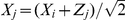is then repeated from parent to child until all nodes have been reached. The scaling factor, , ensures that each has unit variance.

Performance measures

Let (true positive) denote the number of edges correctly identified by the estimated network with (false positive), (false negative), and (true negative) defined similarly. The positive predictive value, 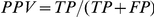, and the sensitivity, , are reported for each estimated network. While it is often customary to include specificity, 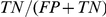, along with and , its conspicuous absence here is for good reason. Since GANs are sparse, is sure to be very large in comparison to . As a result, even a moderate change to will have little influence on the specificity, making this an unsuitable measure of performance.

Simulated Example

This section serves as a prelude to an extensive simulation study, illustrating our methodology by means of a simple example. Specifically, we set and generated a binomial tree and a scale-free tree with , and then simulated an observation dataset from each. In each case, we attempted to recover the true tree from the scaled dataset using our Metropolis-Hastings sampler implemented with 1) , and 2) .

For each chain, the Metropolis-Hastings sampler was run for steps after a burn-in of , starting from the empty network and identity node labeling. The value for the step size, , required for updating the hyperparameters was set to with . As for the hyper-inverse Wishart parameters, we choose which fixes at since the data was standardized. The values of the hyperparameters were recorded at every 'th step after burn-in. The runtime for the Metropolis-Hastings sampler with on a dual GHz PowerPC G5 processor was hrs for the binomial tree and hrs for the scale-free tree. The corresponding runtimes with were hrs and hrs.

The results of the case study are shown in Table 1. In this experiment, our expectation that will recover the scale-free tree more accurately than is confirmed. It should also be noted that was able to recover a reasonable value for the scale-free exponent, too. Not to mention that it recovered the binomial tree on par with , thereby allaying the potential drawback that it would infer a heavy-tailed network, even from binomial data. Remember, this can be explained by the rather large value of . Recall that when is large, actually approximates . And although it may seem odd that fared slightly better on the binomial tree, the disparity falls within the boundaries of sampling variation. More precisely, we ran the Metropolis-Hastings sampler 10 times for each structure prior, starting each run from a different random seed, and found that the standard deviation of the sensitivity was in each case. Finally, we ran the uniform structure prior on both trees, but decided against including the results in Table 1 due to very poor performance.

Table 1. Case study.

		Random Structure Prior		Scale-Free Structure Prior
Topology	True
Binomial	—	0.96	0.59	0.96	0.60
Scale-Free	2.3	0.88	0.54	0.90	0.79

Summary of the networks estimated using (left) and (right) when the true tree topology is binomial in the one case and scale-free with in the other. is the positive predictive value and the sensitivity, which is computed in respect to the the number of edges correctly identified by the estimated network. The value is the estimated scale-free exponent, obtained by averaging over every 'th value in the MCMC chain.

Extended Simulation

Table 2 contains the results of our main simulation. In the previous section, we focused on two particular trees: one binomial, the other scale-free. This time we generated trees () under each model listed in the table together with accompanying datasets of observations. The models listed as scale-free, not including the BA model, and the crumpled one were generated from a two-parameter family of distributions [51]. The parameter setting for generating the crumple trees was and . The simulation settings used for each MCMC run are identical to those of the case study. Finally, the values of , , and reported in the table are averaged over the chains. The simulation was run on the supercomputer, Tsubame [52]. The system has a total of 639 Sun Fire ×4600 nodes. Each node has 8 AMD Opteron Dual Core model 880, 2.4GHz cpus.

Table 2. Full simulation.

		Random Structure Prior		Scale-Free Structure Prior
Topology	True
Binomial	—	0.96	0.59	0.96	0.60	18.70
Scale-Free (BA)	3.0	0.95	0.58	0.94	0.65	2.49
Scale-Free	2.5	0.93	0.56	0.93	0.62	2.35
Scale-Free	2.3	0.86	0.49	0.90	0.71	2.18
Crumple	—	0.76	0.38	0.90	0.80	2.10
Star	—	0.63	0.30	0.90	0.86	2.10

Summary of the networks estimated using (left) and (right) for a variety of topologies. A total of trees of were generated for each kind of topology; each has nodes with an accompanying observation dataset. is the positive predictive value and the sensitivity, which are computed according the the number of edges correctly identified by the estimated network. is the estimated scale-free exponent. The values in the table are averaged over the MCMC runs.

Just as with the simulated example, recovers the binomial trees equally as well as . In fact, the agreed to two decimal places, while the was actually a little higher under the scale-free structure prior. This slight discrepancy can be accounted for by noting that the standard deviation of was for both priors. Also as expected, the more heavy-tailed the underlying trees become, the more outperforms . The difference becomes huge in the extreme case of a star tree. Moreover, demonstrated the ability to roughly recover the scale-free exponent of the underlying tree.

Real Data Example

We demonstrate our methodology on a subset of the gene expression data from a breast cancer study by [40] that was originally analyzed in [25]. The dataset (Dataset S1) consists of expression profiles for genes related to the estrogen receptor gene ESR1 (also known as ER-alpha) derived from tumor samples. This gene is an estrogen-activated transcription factor key to the proliferation of cancerous cells that is found to be overexpressed in luminal type A and B breast cancers. The overall level of ESR1 expression is higher in type A than in type B with the former correlating with better prognosis [53].

The Metropolis-Hastings sampler was run on the standardized data with both the random structure prior and its scale-free counterpart, yielding the corresponding GANs and . For comparison's sake, the edge inclusion threshold, , was tuned for each run so that the resulting GAN comprised exactly edges; the value of is for and for . In both cases, the Metropolis-Hastings sampler was started from the empty network with identity node labeling and iterations were run with the first discarded as burn-in. The hyperparameter assignments were identical to those of the simulated examples. The runtime on a dual GHz PowerPC G5 processor was hrs with and hrs with .

At this stage, comparing the performance of the scale-free structure prior in a broader context is of key importance. To this end, we used the software packages ARACNE [54], [55] and BANJO [23] to analyze the gene expression data as well. ARACNE constructs a relevance network based on estimated mutual information between all pairs genes, but there is a twist. After a relevance network is inferred by connecting any pair of genes with mutual information greater than a certain cutoff value, some edges suspected to represent indirect interactions are eliminated using the data processing inequality principle. We chose the cutoff value to be so that the number of estimated edges was , while all other program arguments were set at their default values. The code itself was run in a matter of minutes. BANJO, on the other hand, constructs a Bayesian network from discrete data using a heuristic search strategy to explore the space of -node, directed networks without cycles. Each network happened upon in the search is ranked using a Bayesian Dirichlet equivalence scoring metric. We discretized the data into three categories and limited the number of parents any given node may have to 10. Once again, all other program arguments were set at their default values. The estimated network, which was found to have directed edges, was the highest scoring network after running BANJO for hr.

Figures 3(A) and (B) show the GANs estimated with and . The latter exhibits clear hubs, supporting the view that a gene regulatory network consists of a small minority of hub genes with the vast majority of genes engaged in a small number of interactions. By contrast, the topology of is relatively decentralized with no single gene dominating the network. Additionally, the estimated value of exponent in the static model was , in line with findings in the literature for gene regulatory networks [31]. Turning now to Figures 3(C) and (D), it is interesting to see that the topology of the relevance network echoes that of the GAN inferred using the scale-free structure prior. The same can be said for the Bayesian network and the random structure prior GAN. Of course, a more exquisite experimental technique is the only sure-fire way to validate the individual regulatory interactions suggested by these graphical models. These results, however, are telltale in one respect. In a study comparing different reconstruction methods on simulated data [56], it was reported that BANJO performs well only when , while ARACNE shows good performance even when .

Figure 3. Estimated networks for the breast cancer expression dataset.

(A) The gene association network estimated with random structure prior, , and (B) the gene association network estimated with the scale-free structure prior, . (C) The relevance network estimated with ARACNE, and (D) the Bayesian network estimated with BANJO. The labeled nodes are the largest hubs as identified by (1:FOXA1, 2:SLC39A6, 3:E2F3). For ease of visualization, only the largest connected subnetworks are displayed.

The topological dissimilarity between the two GANs is again made evident by a visual inspection of their degree distributions, plotted in Figure 4. The most abundantly connected node in has degree , whereas contains four nodes with degree exceeding this value; the largest hubs correspond to the genes FOXA1 (HNF-3A), SLC39A6 (LIV-1), and E2F3 (KIAA0075) and have degree , , and , respectively. The main hub FOXA1 is a forkhead box family transcription factor that is necessary for optimum expression of roughly half of all ESR1-regulated genes [57]. In a recent study [58], it was found that FOXA1 is expressed predominantly in luminal type A carcinomas, making it a potential marker of good prognosis. Previously unrecognized as a hub, SLC39A6 functions as a zinc transporter, and was identified in [59] to be highly expressed in ESR1-positive tumors as well as showing a highly significant association with the spread of breast cancer to the lymph nodes. Meanwhile, E2F3 is a transcription factor that has been shown to regulate numerous genes involved in cell cycle progression [60].

Figure 4. Degree distributions of the gene association networks.

The labels , , and indicate the locations of the genes FOXA1, SLC39A6, and E2F3, respectively. The plots are on a scale.

Finally, both GANs agreed with the relevance network on some established regulatory interactions as can be seen in Figure 5. For instance, FOXA1 is connected to AR (androgen receptor), which is known to regulate estrogen receptor expression [61]. FOXA1 has also been shown to play a direct role in the transcription of the TFF1 (pS2) gene [62], and our work agrees with [24] on the role of TFF3 (ITF) as an intermediary. By contrast, the Bayesian network agreed on very few of these interactions. Part of the explanation is likely to rest in using the maximum posterior network as the estimated network. As we drew attention to in the section Network and Parameter Estimation, a single network of high posterior probability may be a less representative estimator than an network consisting of edges that occur with high frequency in an MCMC chain. Another possible contributing factor is that the number of observations was insufficient for BANJO, but what is also unclear is the extent to which discretizing the expression data affected the quality of the inference.

Figure 5. Gene interactions identified by all methods.

A subnetwork of the gene interactions involved with the estrogen receptor gene, ESR1, that were commonly identified by the random structure prior, , the scale-free structure prior, , and the relevance network (estimated with ARACNE). The directed edges indicate the gene interactions on which the Bayesian network (estimated with BANJO) agreed with the other three methods.

Discussion

The main purpose of this paper has been to introduce a scale-free structure prior, , for graphical models with a view toward the inference of large-scale GANs from datasets consisting of few observations, , for a comparatively large number of variables, . It is important to point out that the true network need not follow a power-law in order for the scale-free prior to be applicable; rather, is a convenient distribution that can account for heavy-tailed degree distributions — a crucial limitation of the random structure prior. That said, we have shown in simulated examples that performs markedly better than the random structure prior at recovering networks characterized by heavy-tailed degree distributions. What is more, proved versatile enough to recover random networks on par with itself. Above all, our analysis of the breast cancer expression data illustrates the practical value of the scale-free structure prior as an instrument to aid in the identification of candidate hub genes with the potential to direct the hypotheses of molecular biologists, and thus drive future experiments.

A node labeling , that is, a permutation of the integers applied to the nodes of so that each is represented by the integer , is an essential prerequisite for any MCMC implementation of the scale-free structure prior. The reason is that the scale-free network model underlying , or any other scale-free network model for that matter, is so elaborate that the nodes are not interchangeable in regard to computing the probability of . And, although easily overshadowed by itself, our new Metropolis-Hastings sampler for is an innovative contribution in its own right. Our sampler uses a simple pair swapping strategy for updating , and one future topic of research is to investigate the comparative performance of more ingenious update schemes. More research is also required in order to assesses how accurately can be estimated.

We take pains to point out that while our implementation is for GGMs, the methodology described here applies to graphical models more generally. For instance, could be applied crudely to Bayesian network inference by simply ignoring edge directionality, or else the underlying static model could be modified to have directed edges. The latter approach raises an interesting consideration: in gene regulatory networks, according to the prevailing wisdom [31], it is actually only the out-degree distribution that follows a power-law. By contrast, the in-degree of a node is usually small and its distribution is better approximated by a sort of restricted exponential function. While this distinction gets blurred when inference is conducted with undirected graphical models, Bayesian networks provide an obvious incentive for taking it into account. Indeed, Bayesian networks may prove to be a more promising area of application because they currently able to handle much larger networks than GGMs [63].

Although the static model is not biologically motivated, it is a defensible choice as an underlying model for on the grounds that it is a simple model with the potential to describe any network topology; not to mention that it includes the ER model as a limiting case. But there is more, implementing a structure prior based on a growing network model poses some added difficulties because not only will the probability of a network depend on the choice of seed network, but evaluating will result in a greater expenditure of computational resources as the edge inclusion probabilities depend on the order in which they were added to the network.

All the same, we implemented two other scale-free structure priors based on growing models; one on the Poisson-growth, preferential attachment model [64], and another on the biologically meaningful duplication model. In the former case, we were able to get away with using a single node as the seed network, and we found that while this prior recovered heavy-tailed networks as well as , yet it understandably struggled to accurately recover random networks. Meanwhile, the duplication model based structure prior was highly sensitive to the choice of seed network in addition to being unstable due to the complexity of the model. One future avenue of research is to adapt these models, or the MCMC implementation, to be more applicable for use as a prior distributions. The primary motivation for doing so is that the model parameters have biological meaning, and their estimation could prove of independent interest.

The estimation of network model parameters has been an incidental aspect of our work; however, it is related to the quite different problem of fitting network models to known biological networks. Likelihood and likelihood-free methods have been developed [65], [66] in order to fit a hybrid preferential attachment/duplication and divergence model to some protein-protein interaction networks, obtaining estimates of the model parameters. These methodologies assume that the ordering of the nodes in time, that is , is known, but in most cases this information is unknown. In the future, our Metropolis-Hastings sampler could very well be applied to this problem.

Software is available from the corresponding author upon request.

Supporting Information

Dataset S1

This file contains the gene expression data that we analyzed in our paper.

(0.05 MB TXT)

References

- 1.Husmeier D. Sensitivity and specificity of inferring genetic regulatory interactions from microarray experiments with dynamic bayesian networks. Bioinformatics. 2003;19:2271–2282. doi: 10.1093/bioinformatics/btg313. [DOI] [PubMed] [Google Scholar]
- 2.West M. Bayesian factor regression models in the “large p, small n” paradigm. Oxford University Press; 2003. pp. 723–732. [Google Scholar]
- 3.Schlitt T, Brazma A. Current approaches to gene regulatory network modelling. BMC Bioinformatics. 2007;8:S9+. doi: 10.1186/1471-2105-8-S6-S9. [DOI] [PMC free article] [PubMed] [Google Scholar]
- 4.Whittaker J. Graphical models in applied multivariate statistics. New York: John Wiley & Sons; 1990. [Google Scholar]
- 5.Lauritzen SL. Graphical models. Oxford Statistical Science Series. New York: Oxford University Press; 1996. [Google Scholar]
- 6.Edwards D. Introduction to graphical modelling. New York: Springer-Verlag; 2000. [Google Scholar]
- 7.Grzegorczyk M, Husmeier D, Werhli AV. Reverse engineering gene regulatory networks with various machine learning methods. In: Emmert-Streib F, Dehmer M, editors. Analysis of Microarray Data. Weinheim: Wiley-VCH; 2008. pp. 101–142. [Google Scholar]
- 8.Markowetz F, Spang R. Inferring cellular networks - a review. BMC Bioinformatics. 2007;8:S5+. doi: 10.1186/1471-2105-8-S6-S5. [DOI] [PMC free article] [PubMed] [Google Scholar]
- 9.Butte AJ, Tamayo P, Slonim D, Golub TR, Kohane IS. Discovering functional relationships between rna expression and chemotherapeutic susceptibility using relevance networks. Proc Natl Acad Sci U S A. 2000;97:12182–12186. doi: 10.1073/pnas.220392197. [DOI] [PMC free article] [PubMed] [Google Scholar]
- 10.Schäfer J, Strimmer K. A shrinkage approach to large-scale covariance matrix estimation and implications for functional genomics. Statistical applications in genetics and molecular biology. 2005;4 doi: 10.2202/1544-6115.1175. [DOI] [PubMed] [Google Scholar]
- 11.Wille A, Bhlmann P. Low-order conditional independence graphs for inferring genetic networks. Statistical Applications in Genetics and Molecular Biology. 2006;5:1. doi: 10.2202/1544-6115.1170. [DOI] [PubMed] [Google Scholar]
- 12.Castelo R, Roverato A, Chickering M. A robust procedure for gaussian graphical model search from microarray data with p larger than n. Journal of Machine Learning Research. 2006;7:2006. [Google Scholar]
- 13.Magwene PM, Kim J. Estimating genomic coexpression networks using first-order conditional independence. Genome Biology. 2004;5:R100. doi: 10.1186/gb-2004-5-12-r100. [DOI] [PMC free article] [PubMed] [Google Scholar]
- 14.Pe'er D, Nachman I, Linial M, Friedman N. Using bayesian networks to analyze expression data. Journal of Computational Biology. 2000;7:601–620. doi: 10.1089/106652700750050961. [DOI] [PubMed] [Google Scholar]
- 15.Imoto S, Higuchi T, Goto T, Tashiro K, Kuhara S, et al. CSB '03: Proceedings of the IEEE Computer Society conference on Bioinformatics. Washington, DC, USA: IEEE Computer Society; 2003. Combining microarrays and biological knowledge for estimating gene networks via bayesian networks. pp. 104–113. [PubMed] [Google Scholar]
- 16.Tamada Y, Kim S, Bannai H, Imoto S, Tashiro K, et al. Estimating gene networks from gene expression data by combining bayesian network model with promoter element detection. Bioinformatics. 2003;19(Suppl 2):11227–11236. doi: 10.1093/bioinformatics/btg1082. [DOI] [PubMed] [Google Scholar]
- 17.Barnard A, Hartemink AJ. PSB '05: Pacific Symposium on Biocomputing. World Scientific; 2005. Informative structure priors: joint learning of dynamic regulatory networks from multiple types of data. pp. 459–470. [PubMed] [Google Scholar]
- 18.Werhli AV, Husmeier D. Reconstructing gene regulatory networks with bayesian networks by combining expression data with multiple sources of prior knowledge. Statistical applications in genetics and molecular biology. 2007;6 doi: 10.2202/1544-6115.1282. [DOI] [PubMed] [Google Scholar]
- 19.Pe'er D, Regev A, Tanay A. Minreg: inferring an active regulator set. Bioinformatics. 2002;18(Suppl 1):S258–S267. doi: 10.1093/bioinformatics/18.suppl_1.s258. [DOI] [PubMed] [Google Scholar]
- 20.Segal E, Shapira M, Regev A, Pe'er D, Botstein D, et al. Module networks: identifying regulatory modules and their condition-specific regulators from gene expression data. Nature Genetics. 2003;34:166–176. doi: 10.1038/ng1165. [DOI] [PubMed] [Google Scholar]
- 21.Schäfer J, Strimmer K. An empirical bayes approach to inferring large-scale gene association networks. Bioinformatics. 2005;21:754–764. doi: 10.1093/bioinformatics/bti062. [DOI] [PubMed] [Google Scholar]
- 22.Meinshausen N, Bhlmann P. High dimensional graphs and variable selection with the lasso. Annals of Statistics. 2006;34:1436–1462. [Google Scholar]
- 23.Yu J, Smith VA, Wang PP, Hartemink AJ, Jarvis ED. Advances to bayesian network inference for generating causal networks from observational biological data. Bioinformatics (Oxford, England) 2004;20:3594–3603. doi: 10.1093/bioinformatics/bth448. [DOI] [PubMed] [Google Scholar]
- 24.Dobra A, Hans C, Jones B, Nevins JR, West M. Sparse graphical models for exploring gene expression data. Journal of Multivariate Analysis. 2004;90:196–212. [Google Scholar]
- 25.Jones B, Carvalho CM, Dobra A, Hans C, Carter C, et al. Experiments in stochastic computation for high-dimensional graphical models. Statistical Science. 2005;20:388–400. [Google Scholar]
- 26.Erdös P, Rényi A. On random graphs. Publicationes Mathematicae. 1959;6:290–297. [Google Scholar]
- 27.Erdös P, Rényi A. On the evolution of random graphs. Publication of the Mathematical Institute of the Hungarian Academy of Sciences. 1960;5:17–61. [Google Scholar]
- 28.Albert R, Barabási AL. Statistical mechanics of complex networks. Reviews of Modern Physics. 2002;74 [Google Scholar]
- 29.Dorogovtsev SN, Mendes JFF. Evolution of networks. Advances in Physics. 2002;51:1070–1187. [Google Scholar]
- 30.Newman MEJ. The structure and function of complex networks. Siam Review. 2003;45:167–256. [Google Scholar]
- 31.Albert R. Scale-free networks in cell biology. J Cell Sci. 2005;118:4947–4957. doi: 10.1242/jcs.02714. [DOI] [PubMed] [Google Scholar]
- 32.Farkas I, Jeong H, Vicsek T, Barabasi, Oltvai ZN. The topology of the transcription regulatory network in the yeast, saccharomyces cerevisiae. Physica A: Statistical Mechanics and its Applications. 2003;318:601–612. [Google Scholar]
- 33.Kim SK, Lund J, Kiraly M, Duke K, Jiang M, et al. A gene expression map for caenorhabditis elegans. Science. 2001;293:2087–2092. doi: 10.1126/science.1061603. [DOI] [PubMed] [Google Scholar]
- 34.Boccaletti S, Latora V, Moreno Y, Chavez M, Hwang D. Complex networks: Structure and dynamics. Physics Reports. 2006;424:175–308. [Google Scholar]
- 35.Bárabasi AL, Albert R. Emergence of scaling in random networks. Science. 1999;286:509–512. doi: 10.1126/science.286.5439.509. [DOI] [PubMed] [Google Scholar]
- 36.Ohno S. Evolution by gene duplication. G. Allen and Unwin; Springer; 1970. [Google Scholar]
- 37.Solé R, Pastor-Satorras R, Smith E, Kepler T. A model of large-scale proteome evolution. Advances in Complex Systems. 2002;5:43–54. [Google Scholar]
- 38.Pastor-Satorras R, Smith E, Solé RV. Evolving protein interaction networks through gene duplication. J Theor Biol. 2003;222:199–210. doi: 10.1016/s0022-5193(03)00028-6. [DOI] [PubMed] [Google Scholar]
- 39.Goh KI, Kahng B, Kim D. Universal behavior of load distribution in scale-free networks. Phys Rev Lett. 2001;87 doi: 10.1103/PhysRevLett.87.278701. [DOI] [PubMed] [Google Scholar]
- 40.West M, Blanchette C, Dressman H, Huang E, Ishida S, et al. Predicting the clinical status of human breast cancer by using gene expression profiles. Proceedings of the National Academy of Sciences of the United States of America. 2001;98:11462–11467. doi: 10.1073/pnas.201162998. [DOI] [PMC free article] [PubMed] [Google Scholar]
- 41.Dempster AP. Covariance selection. Biometrics. 1972;28:95–108. [Google Scholar]
- 42.Wong K, Carter C, Kohn R. Efficient estimation of covariance selection models. Biometrika. 2003;90:809–830. [Google Scholar]
- 43.Guidici P, Green PJ. Decomposable graphical model determination. Biometrika. 1999;86:785–801. [Google Scholar]
- 44.Adamic LA, Huberman BA. Zipf's law and the internet. Glottometrics. 2002;3:143–150. [Google Scholar]
- 45.Lee DS, Goh KI, Khang B, Kim D. Scale-free random graphs and potts model. Pramana Journal of Physics. 2005;64:1149–1159. [Google Scholar]
- 46.Rannala B, Yang Z. Probability distribution of molecular evolutionary trees: a new method of phylogenetic inference. J Mol Evol. 1996;43:304–311. doi: 10.1007/BF02338839. [DOI] [PubMed] [Google Scholar]
- 47.Yang Z, Rannala B. Bayesian phylogenetic inference using dna sequences: a markov chain monte carlo method. Mol Biol Evol. 1997;14:717–724. doi: 10.1093/oxfordjournals.molbev.a025811. [DOI] [PubMed] [Google Scholar]
- 48.Ronquist F, Huelsenbeck JP. Mrbayes 3: Bayesian phylogenetic inference under mixed models. Bioinformatics. 2003;19:1572–1574. doi: 10.1093/bioinformatics/btg180. [DOI] [PubMed] [Google Scholar]
- 49.Frydenberg M, Lauritzen SL. Decomposition of maximum likelihood in mixed interaction models. Biometrika. 1989;76:539–555. [Google Scholar]
- 50.Carvalho LE, Lawrence CE. Centroid estimation in discrete high-dimensional spaces with applications in biology. Proceedings of the National Academy of Sciences. 2008;105:3209–3214. doi: 10.1073/pnas.0712329105. [DOI] [PMC free article] [PubMed] [Google Scholar]
- 51.Burda Z, Correia JD, Krzywicki A. Statistical ensemble of scale-free random graphs. Phys Rev E. 2001;64:046118. doi: 10.1103/PhysRevE.64.046118. [DOI] [PubMed] [Google Scholar]
- 52.Matsuoka S. The road to TSUBAME and beyond, Boca Raton, FL: Chapman & Hall/CRC, chapter 14. 2008. pp. 289–310. Computational Science Series.
- 53.Sørlie T, Perou CM, Tibshirani R, Aas T, Geisler S, et al. Gene expression patterns of breast carcinomas distinguish tumor subclasses with clinical implications. Proceedings of the National Academy of Sciences of the United States of America. 2001;98:10869–10874. doi: 10.1073/pnas.191367098. [DOI] [PMC free article] [PubMed] [Google Scholar]
- 54.Basso K, Margolin AA, Stolovitzky G, Klein U, Dalla-Favera R, et al. Reverse engineering of regulatory networks in human b cells. Nature Genetics. 2005;37:382–390. doi: 10.1038/ng1532. [DOI] [PubMed] [Google Scholar]
- 55.Margolin AA, Nemenman I, Basso K, Wiggins C, Stolovitzky G, et al. Aracne: an algorithm for the reconstruction of gene regulatory networks in a mammalian cellular context. BMC bioinformatics. 2006;7(Suppl 1) doi: 10.1186/1471-2105-7-S1-S7. [DOI] [PMC free article] [PubMed] [Google Scholar]
- 56.Bansal M, Belcastro V, Ambesi-Impiombato A, di Bernardo D. How to infer gene networks from expression profiles. Molecular Systems Biology. 2007;3 doi: 10.1038/msb4100120. [DOI] [PMC free article] [PubMed] [Google Scholar]
- 57.Carroll JS, Brown M. Estrogen receptor target gene: an evolving concept. Molecular Endocrinology. 2006;20:1707–1714. doi: 10.1210/me.2005-0334. [DOI] [PubMed] [Google Scholar]
- 58.Nakshatri H, Badve S. Foxa1 as a therapeutic target for breast cancer. Expert Opinions on Therapeutic Targets. 2007;11:507–514. doi: 10.1517/14728222.11.4.507. [DOI] [PubMed] [Google Scholar]
- 59.Taylor KM. A distinct role in breast cancer for two liv-1 family zinc transporters. Biochemical Society Transactions. 2008;36(Pt6):1247–1251. doi: 10.1042/BST0361247. [DOI] [PubMed] [Google Scholar]
- 60.Giangrande P, Hallstrom T, Tunyaplin C, Calame K, Nevins J. Identification of e-box factor tfe3 as a functional partner for the e2f3 transcription factor. Molecular and Cellular Biology. 2003;23:3707–3720. doi: 10.1128/MCB.23.11.3707-3720.2003. [DOI] [PMC free article] [PubMed] [Google Scholar]
- 61.Sahlin L, Norstedt G, Eriksson H. Androgen regulation of the insulin-like growth factor 1 and the estrogen receptor in rat uterus and liver. Journal of Steroid Biology. 1994;51:57–66. doi: 10.1016/0960-0760(94)90115-5. [DOI] [PubMed] [Google Scholar]
- 62.Beck S, Sommer P, dos Santos Silva E, Blin N, Gött P. Hepatocyte nuclear factor 3 (winged helix domain) activates trefoil factor gene tff1 through a binding motif adjacent to the tata box. DNA Cell Biology. 1999;18:157–164. doi: 10.1089/104454999315547. [DOI] [PubMed] [Google Scholar]
- 63.Hartemink AJ. Reverse engineering gene regulatory networks. Nature Biotechnology. 2005;23:554–555. doi: 10.1038/nbt0505-554. [DOI] [PubMed] [Google Scholar]
- 64.Sheridan P, Yagahara Y, Shimodaira H. A preferential attachment model with poisson growth for scale-free networks. Annals of the Institute of Statistical Mathematics. 2008;60:747–761. [Google Scholar]
- 65.Wiuf C, Brameier M, Hagberg O, Stumpf MP. A likelihood approach to analysis of network data. Proceedings of the National Academy of Sciences of the United States of America. 2006;103:7566–7570. doi: 10.1073/pnas.0600061103. [DOI] [PMC free article] [PubMed] [Google Scholar]
- 66.Ratmann O, Jørgensen O, Hinkley T, Stumpf M, Richardson S, et al. Using likelihood-free inference to compare evolutionary dynamics of the protein networks of h. pylori and p. falciparum. PLoS Computational Biology. 2007;3:2266–2278. doi: 10.1371/journal.pcbi.0030230. [DOI] [PMC free article] [PubMed] [Google Scholar]
Associated Data
This section collects any data citations, data availability statements, or supplementary materials included in this article.
Supplementary Materials