Online prediction of respiratory motion: multidimensional processing with low-dimensional feature learning

Abstract

Accurate real-time prediction of respiratory motion is desirable for effective motion management in radiotherapy for lung tumor targets. Recently, nonparametric methods have been developed and their efficacy in predicting one-dimensional respiratory-type motion has been demonstrated. To exploit the correlation among various coordinates of the moving target, it is natural to extend the 1D method to multidimensional processing. However, the amount of learning data required for such extension grows exponentially with the dimensionality of the problem, a phenomenon known as the ‘curse of dimensionality’. In this study, we investigate a multidimensional prediction scheme based on kernel density estimation (KDE) in an augmented covariate–response space. To alleviate the ‘curse of dimensionality’, we explore the intrinsic lower dimensional manifold structure and utilize principal component analysis (PCA) to construct a proper low-dimensional feature space, where kernel density estimation is feasible with the limited training data. Interestingly, the construction of this lower dimensional representation reveals a useful decomposition of the variations in respiratory motion into the contribution from semiperiodic dynamics and that from the random noise, as it is only sensible to perform prediction with respect to the former. The dimension reduction idea proposed in this work is closely related to feature extraction used in machine learning, particularly support vector machines. This work points out a pathway in processing high-dimensional data with limited training instances, and this principle applies well beyond the problem of target-coordinate-based respiratory-based prediction. A natural extension is prediction based on image intensity directly, which we will investigate in the continuation of this work. We used 159 lung target motion traces obtained with a Synchrony respiratory tracking system. Prediction performance of the low-dimensional feature learning-based multidimensional prediction method was compared against the independent prediction method where prediction was conducted along each physical coordinate independently. Under fair setup conditions, the proposed method showed uniformly better performance, and reduced the case-wise 3D root mean squared prediction error by about 30–40%. The 90% percentile 3D error is reduced from 1.80 mm to 1.08 mm for 160 ms prediction, and 2.76 mm to 2.01 mm for 570 ms prediction. The proposed method demonstrates the most noticeable improvement in the tail of the error distribution.

1. Introduction

Accurate delivery of radiation treatment requires efficient management of intrafractional tumor target motion, especially for highly mobile targets such as lung tumors. Furthermore, prediction is necessary to account for system latencies caused by software and hardware processing (Murphy and Dieterich 2006). Predicting respiratory motion in real time is challenging, due to the complexity and irregularity of the underlying motion pattern. Recent studies have demonstrated the efficacy of semiparametric and nonparametric machine learning techniques, such as neural networks (Murphy and Dieterich 2006), nonparametric local regression (Ruan et al 2007) and kernel density estimation (Ruan 2010). For a given lookahead length, these methods build a collection of covariate/response variable pairs retrospectively from training data and learn the underlying inference structure. The covariate at any given time consists of an array of preceding samples; the response takes on the value after a delay corresponding to the lookahead length, interpolated if necessary. In real-time applications, the testing covariate is constructed online, and the corresponding response value is estimated based on the map/distribution learnt from the training data.

These single-dimensional developments can be trivially extended to process multidimensional data by evoking 1D prediction along each physical coordinate independently. A more natural alternative is to formulate the multidimensional prediction problem directly, using multidimensional training and predictors. In principle, all of the aforementioned techniques apply, yet the involved high-dimensional learning gives rise to the concern known as the ‘curse of dimensionality’ (Bellman 1957)—the amount of data required to learn a map or distribution grows exponentially with the dimensionality of the underlying space. The requirement of mass training data poses a challenge for highly volatile respiratory motion, as rapid changes require fast response from adaptive prediction algorithms with minimal data requirement.

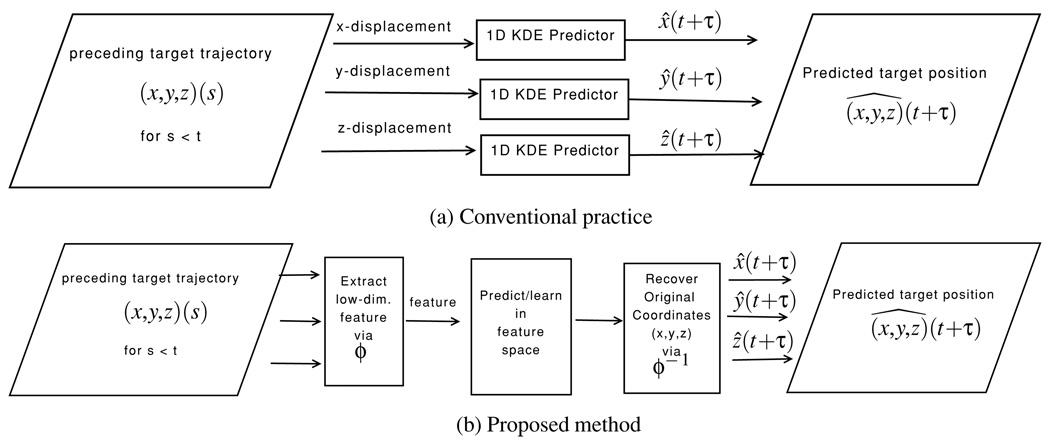
A key observation that allows us to circumvent this difficulty is that most training and testing pairs lie in a sub-manifold of the complete high-dimensional space. This motivates us to study a lower dimensional feature space where the essential topologies of training and testing are preserved. It is natural to expect that efficient regression performed in this feature space produces an ‘image’ of the higher dimensional predictor. To demonstrate the proposed principle, we use the kernel density estimation (KDE)-based prediction method as an example, yet we expect similar behavior for the majority of semiparametric/nonparametric methods. For simplicity, we adopt a simple linear manifold (subspace) spanned by the principal components as the feature space (Gerbrands 1981). A forward mapping first projects all covariate/response pairs into this lower dimensional feature space, which effectively ‘lifts’ the curse of dimensionality for training. The core of the KDE-based prediction is then performed, and the prediction value is mapped back into the original physical space subsequently. Figure 1 summarizes the fundamental difference between the conventional practice where 1D predictors are applied to each coordinate component, respectively, and the proposed method where the multidimensional information is processed as an integrated entity, with low-dimensional feature learning for enhanced performance. We review the KDE-based prediction briefly and present the proposed method in section 2. Section 3 reports the test data, the implementation detail and the results. Section 4 summarizes the study and discusses future research directions.

Figure 1.

Schematic for the conventional practice versus the proposed method. (a) The conventional practice processes each individual coordinate direction independently; (b) the proposed method follows the following steps: (1) mapping the original multidimensional signal trajectory to a lower dimensional feature space; (2) performing prediction in the feature space; (3) mapping the prediction value back to the original coordinates.

2. Methods¹

2.1. Background for KDE-based prediction

Let s(t) ∈ ℛ³ denote the spatial coordinate of the target at time t, and the goal of predicting τ time units ahead is to estimate s(t + τ) from (sampled) trajectory {s(r)|r ≤ t} at preceding times. We consider a length 3p covariate variable x_t = [s(t − (p − 1)Δ), s(t − (p − 2)Δ),…, s(t)] and response y_t = s(t + τ), where the parameter Δ determines the ‘lag length’ used to augment the state for capturing the system dynamics. At any specific time point t, one could retrospectively generate a collection of covariate-response pairs z_r = (x_r, y_r) ∈ ℛ^3(p+1) for r < t − τ, which are regarded as independent observations of a random vector Z = (X, Y) ∈ ℛ^3(p+1). The distribution of Z can be estimated with KDE from {z_r} with p_Z(z) = Σ_r κ(z; z_r) where κ(z; z_r) is the kernel distribution centered at z_r. Now, given the testing covariate variable x_t, one can find the conditional distribution of p_Y|X(y|X = x_t) and subsequently obtain an estimate of y_t.

When the Gaussian kernel and the mean estimate are used to estimate the joint density and to generate the prediction, respectively, the KDE-based method is given in algorithm 1.

Algorithm 1.

Predict ŷ from (x_r, y_r) with Gaussian kernel and mean estimate.

Determine covariance Σx and σy for covariate and response variables. Compute the weights according to $$w_r=\text{exp}[-{(\mathit{x}-{\mathit{x}}_r)}^T{\displaystyle {\sum }_{\mathit{x}}^{-1}(\mathit{x}-{\mathit{x}}_r)],}$$ (1) Compute the mean estimate ${\widehat{\mathit{y}}}_{\text{mean}}=\frac{w_r{\mathit{y}}_r}{{\mathrm{\Sigma }}_r{w}_r}.$

Recall that one does not need to compute the conditional distribution explicitly when the mean estimate is used, due to the interchangeability of linear operations. Geometrically, w_r characterizes the ‘distance’ between the testing covariate and the rth training covariate, and the final estimate y_t is a convex combination of the training response y_r’s, weighted by w_r.

2.2. Low-dimensional feature learning

Even though algorithm 1 does not require explicit computation of the probability distributions, the underlying logic relies on estimating the joint probability distribution of the covariate-response variables. In general, a large number of samples are necessary to perform kernel density estimation in ℛ^3(p+1). However, correlation among various dimensions of the covariate makes it highly likely that the probability distribution concentrates on a sub-manifold in this high-dimensional space. This motivates us to seek amap ϕ : ℛ^3(p+1) → ℛ_q, with q < 3(p+1), which takes points in the original 3(p + 1) ambient space to a feature space of a much lower dimension. Considering the presence of noise in the original data, we only require this map to preserve most of the information.

As there is no requirement for a tight embedding, i.e. the feature space is allowed to have a higher dimension than the intrinsic manifold, we assume a separable kernel with respect to the projection of covariate and response variables in the feature space, in order to preserve the simple algorithmic structure in algorithm 1. Mathematically, this means the feature map ϕ has an identity component and can be represented as

$$\varphi (\mathit{x},\mathit{y})=\left[\begin{array}{cc}\tilde{\varphi }\hfill & 0\hfill \\ 0\hfill & I\hfill \end{array}\right](\mathit{x},\mathit{y})=(\tilde{\mathit{x}},\mathit{y}).$$

For simplicity, we consider only linear maps for ϕ̃. Motivated by the geometric interpretation of algorithm 1, we want x̃ to preserve the relative ‘distance’ among points in the space. A natural choice for a low-dimensional and almost isometric map is the projection onto the subspace spanned by the (major) principal components. Let the eigen decomposition of Σ_x ∈ ℛ^3p×3p be

$${\mathrm{\Sigma }}_{\mathit{x}}=V\text{diag}\{{\lambda }_j\}V\prime ,$$

where V is an orthogonal matrix and λ_j ≥ 0 ∀ j. Upon determining the dimensionality m of the feature space by examining the decay pattern of λ_j, we project the training covariates x onto the feature space by taking the inner product between x and the columns of V, i.e.

$${\tilde{\mathit{x}}}_i=\langle \mathit{x},{\mathit{\upsilon }}_i\rangle ,$$

where υ_i is the column of V corresponding to the ith largest eigenvalue λ_i, for i = 1, 2, …, m.

By substituting the distance between the testing covariate and the training covariates with the distance between their projections in the principal space, algorithm 1 can be easily modified to yield algorithm 2 for multidimensional prediction with low-dimensional feature learning.

Algorithm 2.

Multidimensional prediction with low-dimensional KDE-based feature learning.

Estimate covariance Σx from the training covariates. Perform eigen decomposition on Σx and define the projection matrix P with columns being the first m principal components. $$\begin{array}{cccc}{\mathrm{\Sigma }}_{\mathit{x}}=V\text{diag}\{{\lambda }_j\}V\prime ,\hfill & P(:,i)=V(:,i)\hfill & \text{for}\hfill & i=1,2,\dots ,m.\hfill \end{array}$$ Project the training and testing covariates onto the subspace by $$\begin{array}{cc}{\tilde{\mathit{x}}}_r=P\prime {\mathit{x}}_r\forall r;\hfill & \tilde{\mathit{x}}=P\prime \mathit{x}.\hfill \end{array}$$ Compute the weights according to $$w_r=\text{exp}[-\beta {\Vert \tilde{\mathit{x}}-{\tilde{\mathit{x}}}_r\Vert }^2],$$ (2) where β is a preset parameter inversely proportional to the kernel bandwidth. Compute the mean estimate ${\widehat{\mathit{y}}}_{\text{mean}}=\frac{w_r{\mathit{y}}_r}{{\mathrm{\Sigma }}_r{w}_r}.$

2.3. Technical remarks

• In general, it is difficult to determine the number of principal components to keep (m in algorithm 2). Fortunately, the spectrum of 3D respiratory trajectories (e.g. (3)) presents a clear and sharp cutoff. Intuitively, when the physical coordinates are strongly correlated, it is expected that the intrinsic dimensionality of the feature space would be close to the dimensionality of a single physical coordinate m ≈ p, from which the other two coordinates can be inferred. This observation is supported with experimental data in section 3.

• As in the case of a 1D KDE, the parameter p controls the number of augmented states, thus the order of dynamics for inference. It is necessary that p ≥ 2 to capture the hysteresis of the respiratory motion. On the other hand, choosing a large p implies a higher dimensional feature space and requires more training sample as a consequence. From our experience, p = 3 offers a proper tradeoff for describing dynamics without suffering the ‘curse of dimensionality’. Similarly, the choice of the lag length Δ reflects the tradeoff between capturing dynamics and being robust toward observation noise. Following a similar philosophy as (Ruan et al 2008), it can be shown that the specific choice of Δ has only a marginal effect on the prediction performance.

• Algorithm 2 uses an identity scaling β⁻¹I for kernel covariance, as opposed to the Σ_x in algorithm 1. This is because the PCA step provides a natural means to distinguish between two different contributors to data variation: the major variations due to the semiperiodic dynamics and the minor variations due to random noise. The former distributes the training covariate x_t samples to different places in the ambient space based on their dynamic state, and the latter associates noise-induced uncertainty with each sample. Therefore, the logical way to set the kernel covariance is to use the covariance estimate in the minor component. As random noise is typically isotropic, it is reasonable to use a scaled identity matrix for kernel covariance. Algorithm 1 does not have access to this decomposition information, and the scaled data covariance is just a ‘poor man’s method’ to select a reasonable kernel covariance.

• An estimate for Σ_x can be obtained by taking the empirical covariance of the training covariate values. As the training covariate-response collection gets updated in real-time, recomputing Σ_x and its eigen decomposition at each instant could be computationally expensive. Note, however, that gradual updates in the training collection only cause mild perturbation in the covariance estimate, with aminimal impact on the energy concentration directions. With these observations, it is feasible to update the principal space much less frequently than updating the training set—in fact, it is reasonable to use a static principal space in most situations.

• Temporal discounting can be incorporated in algorithm 2 exactly the same way as in Ruan (2010). We omit the discussion here to focus on the low-dimensional feature-based KDE learning in multidimensional prediction.

3. Experimental evaluation and result analysis

3.1. Data description

To evaluate the algorithm for clinically relevant intrafraction motion, patient-derived respiratory motion traces were acquired. 159 datasets were obtained from 46 patients treated with radiosurgery on the Cyberknife Synchrony system at Georgetown University under an IRB-approved study (Suh et al 2008). The displacement range for a single dimension was from 0.7 mm to 72 mm. To avoid the complexity of accounting for varying data lengths in generating population statistics, we only use the first 60 s of data from each trajectory in our tests.

3.2. Experimental details and results

3.2.1. Experimental setup

We tested the proposed method with two sets of lookahead lengths. It has been previously determined that a DMLC tracking system has a system response time of 160 ms with Varian RPM optical input (Keall et al 2006), and a response time of 570 ms with a single kV image guidance, accounting for all image processing time (Poulsen et al 2010). The covariate variable is composed of three states (p = 3), with approximately half a second in between (Δ ≈ 0.5 s). The training data consist of covariate-response pairs constructed from observations in the most recent 30 s. When samples are obtained at f Hz, this corresponds to (30 − (p − 1)Δ − τ)f covariate-response pairs. For baseline comparison, we generated KDE-based prediction results along each individual coordinate according to algorithm 1, with kernel covariance independently calculated, under the same configuration condition.

The dimensionality of the feature space is obtained by finding the cutoff points in the spectrum of the training covariate covariance. An obvious cutoff is almost always present, due to the intrinsic difference in pattern and scale between system dynamics and observation noise. This behavior is illustrated with a case study in section 3.2.4 (cf equation (3))

The performance of the prediction algorithm was evaluated retrospectively with the Euclidean distance between the predicted and the observed positions in 3D. For each case, the root mean squared error (RMSE) was also computed and used as one sample in the paired Student’s t-test to compare the performance between independent prediction along each individual coordinate and the proposed method.

3.2.2. Pointwise prediction error analysis

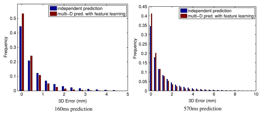
Figure 2 reports the histogram of the pointwise error. Qualitatively, the proposed method results in prediction errors more concentrated in the small end, with sharper dropoff and narrower tails, compared to predicting each coordinate independently. Table 1 corroborates the same observation quantitatively.

Figure 2.

Histogram of the pointwise 3D Euclidean prediction error. Left column: lookahead 160 ms; right column: lookahead 570 ms.

Table 1.

Statistical summary of the pointwise prediction error (in mm).

	160 ms lookahead		570 ms lookahead
Statistics	Independent prediction	Multi-D prediction w/ feature	Independent prediction	Multi-D w/ feature
Mean	0.76	0.52	1.16	0.88
90% percentile	1.80	1.08	2.76	2.01
95% percentile	2.43	1.48	3.67	2.82

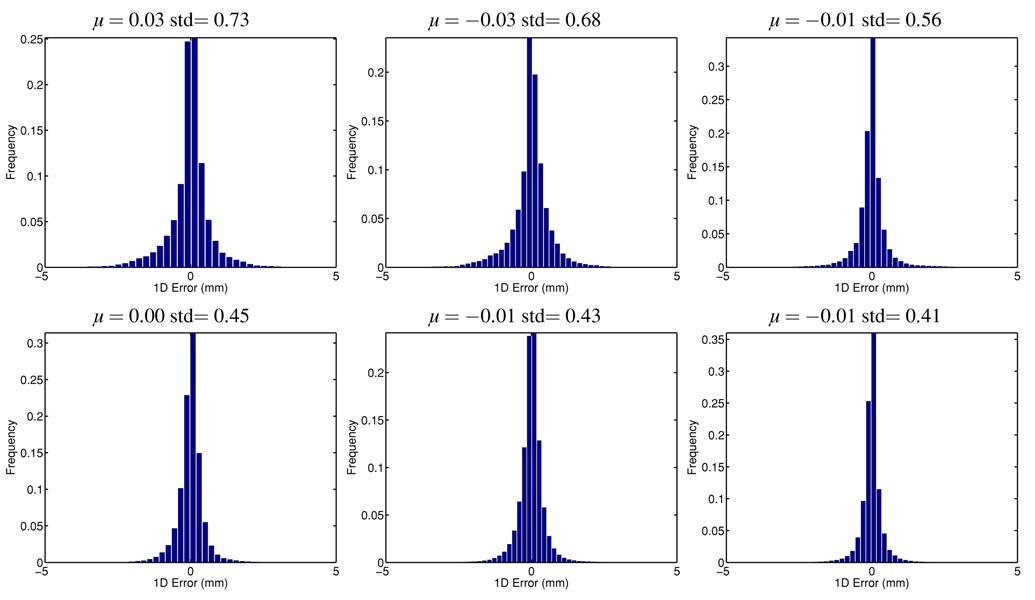
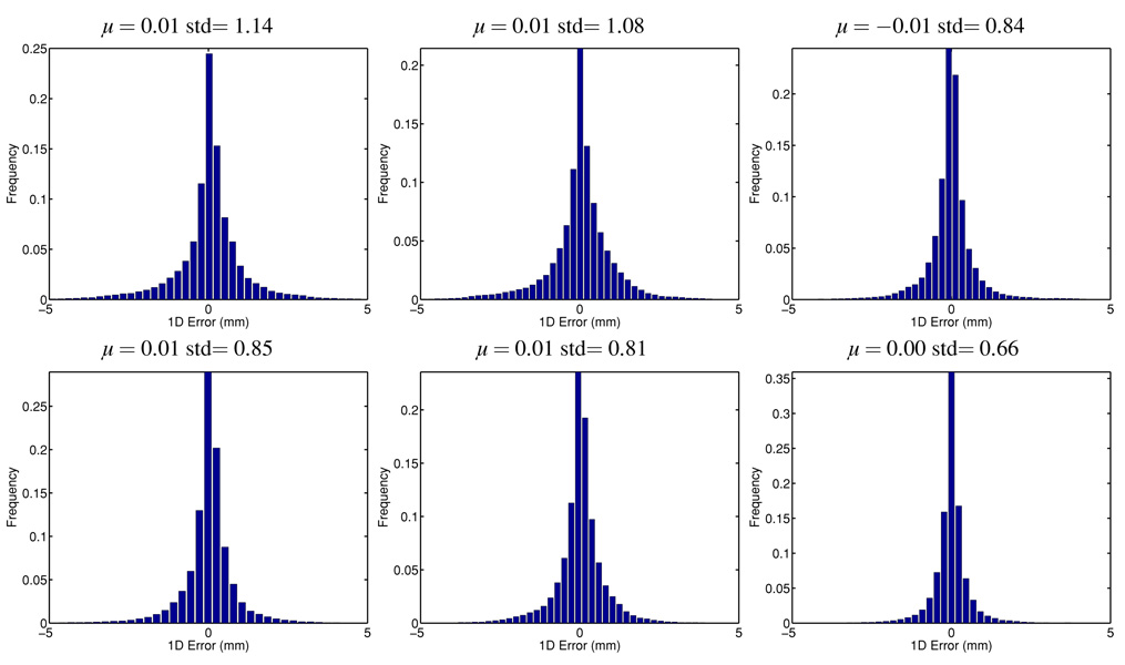
To study the bias and variance of the predictions, we also recorded the 3D vector prediction error and plotted the directional error histogram in figures 3 and 4. Tables 2 and 3 report the mean, standard deviation (std), central 90% and 95% quantiles for each of the x, y, z coordinate. Both methods are unbiased for different lookahead lengths, but the proposed multidimensional method with a low-dimensional feature learning method provides uniformly smaller standard deviation with about 40% reduction, resulting in less prediction error overall. The quantile analysis presented in tables 2 and 3 also shows that the proposed method provides prediction values that are much more concentrated around the true values, reducing the quantile edge values by 30%.

Figure 3.

Histogram of the pointwise error in each direction for 160 ms lookahead prediction. Top row: prediction along each individual direction; bottom row: multidimensional prediction with low-dimensional feature learning. Each column represents a different direction.

Figure 4.

Histogram of the pointwise error in each direction for 570 ms lookahead prediction. Top row: prediction along each individual direction; bottom row: multidimensional prediction with low-dimensional feature learning. Each column represents a different direction.

Table 2.

Statistical summary of the pointwise error (in mm) in each coordinate for 160 ms lookahead prediction.

	Independent prediction			Multi-D prediction w/ feature learning
Statistics	x	y	z	x	y	z
Mean	−0.0298	−0.0260	−0.0122	−0.0005	−0.0061	−0.0085
std	0.73	0.68	0.56	0.45	0.43	0.41
90% quantile	(−1.27 0.97)	(−1.21 0.92)	(−0.77 0.67)	(−0.70 0.61)	(−0.67 0.60)	(−0.54 0.50)
95% quantile	(−1.75 1.41)	(−1.64 1.27)	(−1.12 1.05)	(−0.96 0.87)	(−0.93 0.83)	(−0.78 0.74)

Table 3.

Statistical summary of the pointwise error (in mm) in each coordinate for 570 ms lookahead prediction.

	Independent prediction			Multi-D prediction w/ feature learning
Statistics	x	y	z	x	y	z
Mean	0.0119	0.0081	−0.0053	0.0134	0.0125	−0.0011
Std	1.14	1.08	0.84	0.85	0.81	0.66
90% quantile	(−1.85 1.64)	(−1.81 1.53)	(−1.16 1.04)	(−1.26 1.19)	(−1.28 1.19)	(−0.87 0.82)
95% quantile	(−2.68 2.32)	(−2.58 2.01)	(−1.65 1.61)	(−1.84 1.75)	(−1.82 1.61)	(−1.29 1.26)

3.2.3. Case-wise root mean squared error (RMSE)

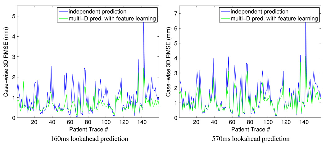
Because of variations in individual respiratory patterns, it is necessary to examine the cases where large prediction error occurs in detail. We computed the case-wise 3D root mean squared prediction error (RMSE) for independent prediction along individual coordinates and the proposed method of multidimensional prediction with low-dimensional feature learning, both based on KDE (figure 5). The proposed method yields almost uniformly lower RMSE: it has similar performance to the independent prediction method in the low error regions but demonstrates its advantage for the more challenging cases. With paired Student’s t-test, the null hypothesis was rejected with strong evidence for prediction lookahead lengths 160 ms and 570 ms, with p-values of 3.5 × 10⁻¹⁴ and 9.2 × 10⁻¹⁵, respectively.

Figure 5.

Comparison of the case-wise 3D RMSE. Left column: lookahead 160 ms; right column: lookahead 570 ms.

3.2.4. An individual case study and its implications

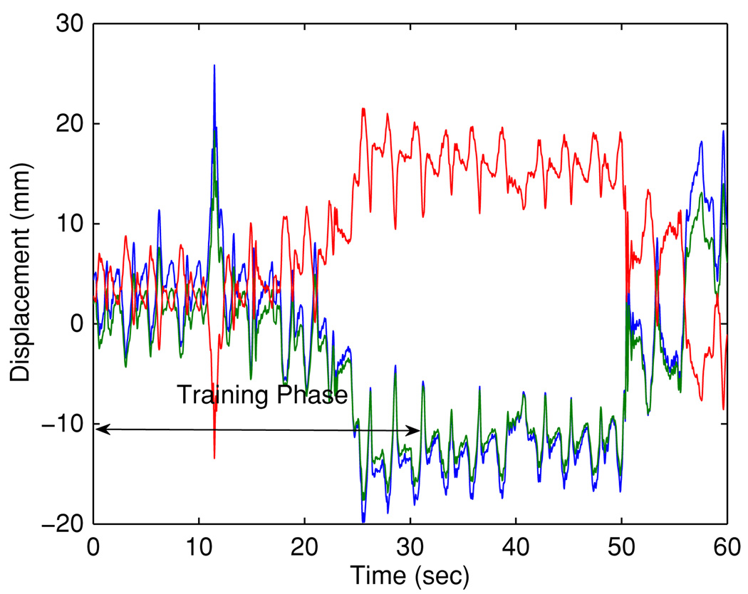
To better understand the behavior of the algorithm, we have closely examined the cases with relatively high prediction errors and present the results for case #142 here. Figure 6 illustrates the respiratory trace. The 3D RMSE with independent prediction are 5.01 mm and 7.18 mm for 160 ms and 570 ms, respectively, and reduce to 2.45 mm and 4.11 mm by the proposed method.

Figure 6.

Respiratory trajectory: samples from the most recent 30 s were used as training data for the KDE. (x, y, z) data are depicted in blue, green and red, respectively.

The eigen decomposition from the initial training yields the following eigenvalue/vectors:

$$\begin{array}{c}{e}_1=474.65,{\mathit{\upsilon }}_1=[-0.38-0.310.29-0.39-0.320.30-0.39-0.310.30];\hfill \\ e_2=35.71,{\mathit{\upsilon }}_2=[0.470.38-0.360.010.01-0.01-0.47-0.380.36];\hfill \\ e_3=23.30,{\mathit{\upsilon }}_3=[-0.28-0.230.220.540.44-0.42-0.27-0.220.21];\hfill \\ e_4=0.01,{\mathit{\upsilon }}_4=[0.300.090.490.300.090.490.290.090.48];\hfill \\ e_5=e_6=e_7=e_8=e_9\approx 0.\hfill \end{array}$$ (3)

A sharp cutoff after the third component is clear in the spectrum. Note that the ith coordinate of the projection x̃ is given by x̃_i = 〈x, υ_i〉, the inner product between the original covariate and the eigenvector. By identifying the corresponding components in x and collecting terms, the first feature component reads

$${\tilde{x}}_1(t)\approx -0.39[x(t-2\tau )+x(t-\tau )+x(t)]-0.31[y(t-2\tau )+y(t-\tau )+y(t)]+0.30[z(t-2\tau )+z(t-\tau )+z(t)].$$ (4)

The summation along each individual coordinate acts as a low pass filter that captures the mean trend. The sign change in the weighting for z from those for x and y captures the opposite trends (or roughly a half-cycle offset). It is quite clear that the first feature component x̃₁ describes the zeroth-order dynamics—drift.

Analogously, the second feature component reads

$${\tilde{x}}_2\approx -0.47[x(t)-x(t-2\tau )]-0.38[y(t)-y(t-2\tau )]+0.36[z(t)-z(t-2\tau )].$$ (5)

Recall that the first-order differential operation can be approximated with the three-stencil difference form $u\prime (t)\approx \frac{u(t)-u(t-2\mathrm{\Delta })}{2\mathrm{\Delta }}$. The difference term along each coordinate corresponds to a differential operation, as in calculating numerical velocity. The change of sign across coordinates can be interpreted the same as in the x̃₁. In summary, the second feature component x̃₂ encodes the (collective) first-order dynamics—velocity.

The third projection component can be rewritten approximately as

$${\tilde{x}}_3\approx -0.27[x(t)+x(t-2\tau )-2x(t-\tau )]-0.22[y(t)+y(t-2\tau )-2y(t-\tau )]+0.21[z(t)+z(t-2\tau )-2z(t-\tau )].$$ (6)

Recall $u″(t)\approx \frac{u(t)+u(t-2\mathrm{\Delta })-2u(t-\mathrm{\Delta })}{{\mathrm{\Delta }}^2}$, and we recognize that the difference in (6) along each individual coordinate captures the second-order differential information. Therefore, the third feature component x̃₃ encodes the second-order dynamics—acceleration.

The sharp cutoff occurs after the third component, and there is no longer clear physical interpretation for other eigenvectors. It is reasonable to conjecture that the energy in e_k, for 4 ≤ k ≤ 9, is induced by observation noise.

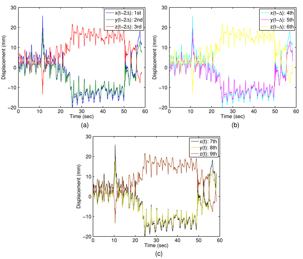
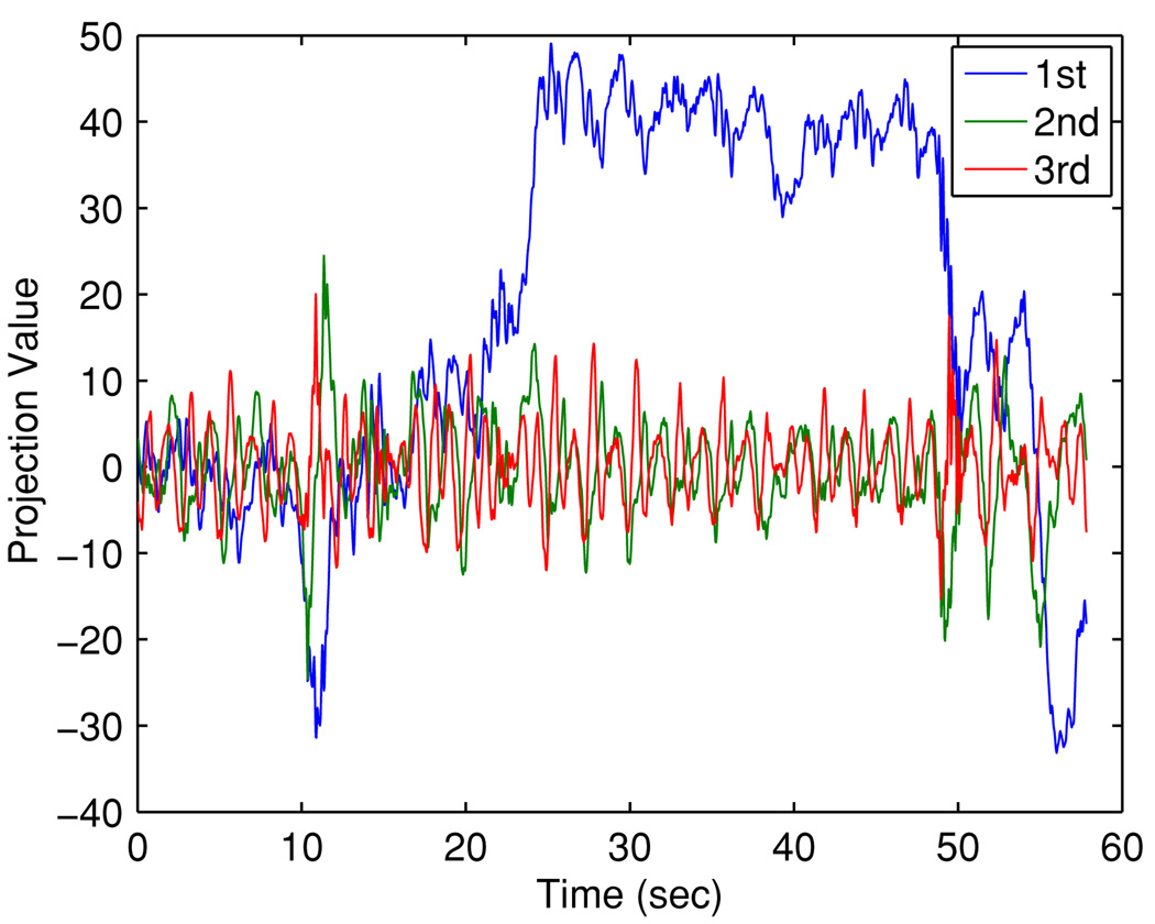
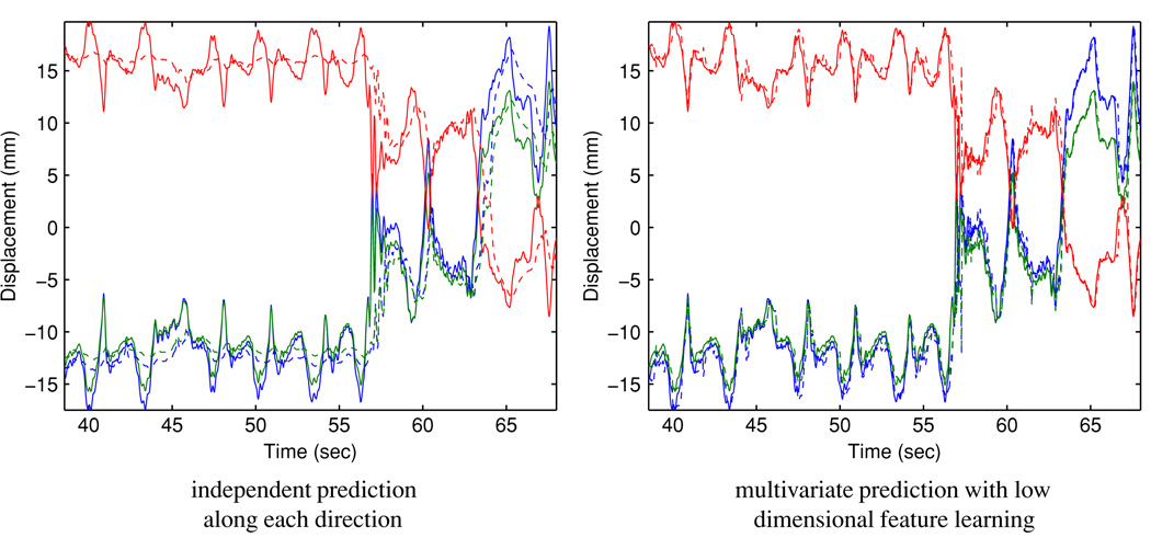
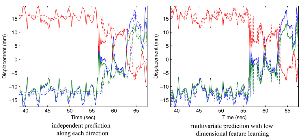
This analysis supports the use of a three-dimensional feature space. Figures 7 and 8 illustrate the original covariate and the projected covariate trajectories, respectively. It can be seen that the major challenge is the large mean drifts in all covariate components—this poses a major obstacle for direct learning in the original space for all methods, as the predictor may have ‘never seen’ any training covariate that ‘resembles’ the testing covariate. In contrast, the projected covariate has one component that clearly captures the mean drift and the other components reflect consistency in first- and second-order dynamics, making it more feasible for the KDE-based method to identify similarity between the testing covariate and a subset of the training covariates. Figure 9 and figure 10 report the prediction results for 160 ms and 570 ms lookahead lengths, respectively.

Figure 7.

Covariate trajectories in the 3D ambient physical space: (a) trajectories of first, second and third covariate; (b) trajectories of fourth, fifth and sixth covariate; (c) trajectories of seventh, eighth and ninth covariate.

Figure 8.

Trajectories of covariate x̃₁, x̃₂ and x̃₃ in the feature space.

Figure 9.

Comparison of 160 ms ahead prediction results. Solid line: observed target position; dashed line: predicted target position. Red: superior–inferior displacement; blue: anterior–posterior displacement; green: left–right displacement.

Figure 10.

Comparison of 570 ms ahead prediction results. Solid line: observed target position; dashed line: predicted target position. Red: superior–inferior displacement; blue: anterior–posterior displacement; green: left–right displacement.

3.3. Discussion

• The sharp cutoff in the spectrum of the training covariance provides strong evidence for the dimensionality of the feature space. Furthermore, the physical interpretation of the principal directions (drift, velocity, acceleration) indicates the universality of the feature space, which justifies the use of the same feature space throughout the trace, rather than recalculating a different projection for every training set update. The linear forward and backward mapping with the principal vectors requires only ~ O(p) FLOPs for each prediction in addition to a 1D KDE-based prediction, whose computation time is negligible compared with the overall system latency.

• The efficacy of the KDE-based prediction along an individual coordinate has been shown in Ruan (2010). The fact that the proposed method compares favorably to this already high-performance benchmark demonstrates the validity of the dimension reduction rationale. Furthermore, the proposed method provides uniform improvement, presenting itself as an ‘all-winner’ in various situations. This is also reflected in the paired Student’s t-test results, where the p-values for both prediction lengths were in the order of 10⁻¹⁵ 10⁻¹⁴.

• Feature extraction is a technique widely used in support vector machine (SVM) learning. Our method differs from SVM learning in that the complexity of kernel density estimation in high-dimensional space drives us to consider a feature space that is lower in dimension than the original one, as opposed to higher dimensional embedding in SVM. We lose information with the projection, but benefit by better utilizing the remaining information in the reduced feature space. In general, the feature map ϕ can be nonlinear, a central topic in nonlinear manifold learning, and techniques such as local linear embedding (LLE) (Roweis and Saul 2000), isomap (Tenenbaum et al 2000) may be used. We feel that the extra complexity associated with nonlinear embedding can be hardly justified in the present system setup, given the success of the current algorithm; yet they may be useful for other motion input/output, such as fully image-based monitoring.

• As mentioned in the introduction, kernel density estimation in the original covariate-response space requires much more training data. Otherwise, there is a risk of the testing covariate falling into a ‘probability vacuum’, with no training covariates close by, resulting in artificial prediction values and large errors.

4. Conclusion and future work

Multivariate prediction is a natural framework to study respiratory motion that has correlation across different spatial coordinates. This paper proposes a simple method to map the high-dimensional covariate variables into a lower dimensional feature space using principal component analysis, followed by kernel density estimation in the feature space. This method manages to alleviate the data requirement for estimation in high-dimensional space, effectively lifting the ‘curse of dimensionality’. Furthermore, close examination of the eigenvalues and eigenvectors from the PCA yields physical interpretations of the feature space and provides a natural separation of the system dynamics from the observation noise. The efficacy of the proposed method has been demonstrated by predicting for various lookahead lengths with patient-derived respiratory trajectories. The feature extraction-based multidimensional prediction method outperforms prediction along individual coordinates almost uniformly, with a clear advantage for the ‘hard-to-predict’ cases. The additional improvement in narrowing the tail of the error distribution over the already high-performance benchmark KDE method promises universally small prediction errors. On a methodological level, this work points out a direction in efficiently processing and learning with high-dimensional data, a common problem in medical signal processing.

The proposed method is now being integrated into a prototype experimental DMLC tracking system at Stanford University. As new observations are acquired, the instantaneous prediction error can be evaluated and heuristics of change detection and management mechanism (such as beam pause) is being investigated. The proposed method will be applied to various real-time monitoring modalities, including Varian RPM optical, Calypso electromagnetic and combined kV/MV image guidance. When fluoroscopic images are taken as input, the low-dimensional feature-based learning provides a pathway toward processing the image data directly, as opposed to the current practice where only extracted marker positions are pipelined into the prediction module. Direct image intensity-based prediction will be the focus of future investigations.

It is also natural to extend the application of the proposed method to radiosurgery and high intensity focused ultrasound treatment, where real-time target localization is crucial for surgery/delivery accuracy.

References

- Bellman RE. Dynamic Programming. Princeton, NJ: Princeton University Press; 1957. [Google Scholar]
- Gerbrands JJ. On the relationships between SVD, KLT, and PCA. Pattern Recognit. 1981;14:375–381. [Google Scholar]
- Keall PJ, Cattell H, Pokhrel D, Dieterich S, Wong KH, Murphy MJ, Vedam SS, Wijesooriya K, Mohan R. Geometric accuracy of a real-time target tracking system with dynamic multileaf collimator tracking system. Int. J. Radiat. Oncol. Biol. Phys. 2006;65:1579–1584. doi: 10.1016/j.ijrobp.2006.04.038. [DOI] [PubMed] [Google Scholar]
- Murphy MJ, Dieterich S. Comparative performance of linear and nonlinear neural networks to predict irregular breathing. Phys. Med. Biol. 2006;51:5903–5914. doi: 10.1088/0031-9155/51/22/012. [DOI] [PubMed] [Google Scholar]
- Poulsen P, Cho B, Ruan D, Sawant A, Keall PJ. Dynamic multileaf collimator tracking of respiratory target motion based on a single kilovoltage imager during arc radiotherapy. Int. J. Radiat. Oncol. Biol. Phys. 2010 doi: 10.1016/j.ijrobp.2009.08.030. at press (doi: 10.1016/j.ijrobp.2009.08.030) [DOI] [PubMed] [Google Scholar]
- Roweis S, Saul L. Nonlinear dimensionality reduction by locally linear embedding. Science. 2000;290:2323–2326. doi: 10.1126/science.290.5500.2323. [DOI] [PubMed] [Google Scholar]
- Ruan D. Kernel density estimation based real-time prediction for respiratory motion. Phys.Med. Biol. 2010;55:1311–1326. doi: 10.1088/0031-9155/55/5/004. [DOI] [PubMed] [Google Scholar]
- Ruan D, Fessler JA, Balter JM. Real-time prediction of respiratory motion based on nonparametric local regression methods. Phys. Med. Biol. 2007;52:7137–7152. doi: 10.1088/0031-9155/52/23/024. [DOI] [PubMed] [Google Scholar]
- Ruan D, Fessler JA, Balter JM, Berbeco RI, Nishioka S, Shirato H. Inference of hysteretic respiratory tumour motion from external surrogates: a state augmentation approach. Phys. Med. Biol. 2008;53:2923–2936. doi: 10.1088/0031-9155/53/11/011. [DOI] [PubMed] [Google Scholar]
- Suh Y, Dieterich S, Cho B, Keall PJ. An analysis of thoracic and abdominal tumour motion for stereotactic body radiotherapy patients. Phys. Med. Biol. 2008;53:3623–3640. doi: 10.1088/0031-9155/53/13/016. [DOI] [PubMed] [Google Scholar]
- Tenenbaum JB, de Silva V, Langford JC. A global geometric framework for nonlinear dimensionality reduction. Science. 2000:2319–2323. doi: 10.1126/science.290.5500.2319. [DOI] [PubMed] [Google Scholar]