Coherent Multidimensional Optical Spectroscopy of Excitons in Molecular Aggregates; Quasiparticle versus Supermolecule Perspectives

1. Introduction

Molecular aggregates are abundant in nature; they form spontaneously in concentrated solutions and on surfaces and can be synthesized by supramolecular chemistry techniques.^1–3 Assemblies of chromophores play important roles in many biological processes such as light-harvesting and primary charge-separation in photosynthesis.⁴ Aggregates come in various types of structures: one-dimensional strands (H and J aggregates),^2,5 two-dimensional layers,^6–8 circular complexes,⁹ cylindrical nanotubes, multiwall cylinders and supercylinders,^10–12 branched fractal structures, dendrimers, and disordered globular complexes.¹³ They also can be fabricated on substrates by “dip-pen” technology.¹⁴ Figure 1 presents some typical structures of pigment-protein complexes found in natural light-harvesting membranes. These are made of chlorophyll and carotenoid chromophores held together by proteins.^4,9,15,16

Figure 1.

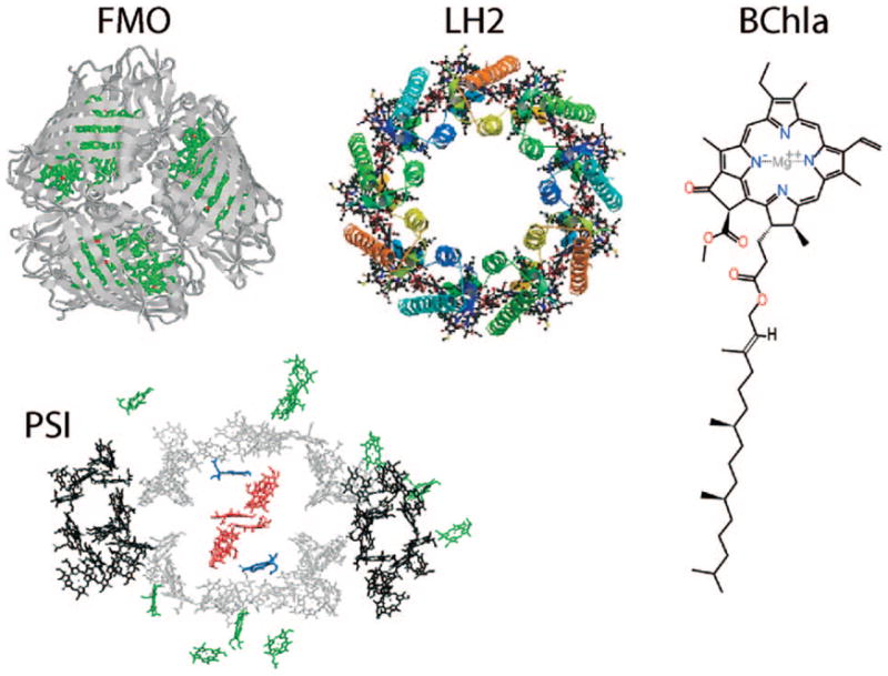
Some biophysical photosynthetic systems: FMO = Fenna-Matthews-Olson protein, a trimer, each unit has 7 chromophores; LH2 = light-harvesting complex 2, double-ring structure of chromophores, 27 chromophores; PS1 = photosystem 1, a complex of 96 chromophores; BChla = bacteriochlorophyll a, a key chromophore in photosynthetic antennae.

We consider aggregates made out of chromophores with nonoverlapping charge distributions where intermolecular couplings are purely electrostatic. The optical excitations of such complexes are known as Frenkel excitons.^17–20 Applications of molecular exciton theory to dimers^4,21–24 show some key features shared by larger complexes. Their absorption spectra have two bands, whose intensities and Davydov splitting are related to the intermolecular interaction strength and the relative orientation.

Excitons in large aggregates can be delocalized across many chromophores and may show coherent or incoherent energy transfer. The optical absorption, time-resolved fluorescence, and pump-probe spectra in strongly coupled linear J-aggregates have been extensively studied.^{2,5,18,25–29} These spectra contain signatures of cooperative optical response: the absorption splits into several Davydov sub-bands and is shifted compared to the monomer. Additionally, the absorption and fluorescence bands are narrower in strongly coupled J aggregates because of motional and exchange narrowing that dynamically average these properties over the inhomogeneous distribution of energies.³⁰ Aggregates may show cooperative spontaneous emission, superradiance, which results in shorter radiative lifetime than the monomer.^31–36 Large molecular aggregates may show several optical absorption bands¹² whose shapes and linewidths depend on their size and geometry. They undergo elaborate multistep energy-relaxation pathways that can be monitored by time-resolved techniques. These pathways are optimized in natural photosynthetic antennas to harvest light with high speed and efficiency.^4,37–41 Exciton energy and charge transport, as well as relaxation pathways, are of fundamental interest. Understanding their mechanisms may be used toward the development of efficient, inexpensive substitutes for semiconductor devices.

Nonlinear optical four-wave mixing (FWM) techniques have long been used for probing inter- and intramolecular interactions, excitation energies, vibrational relaxation, and charge-transferpathwaysinmolecularaggregates.Pump-probe, transient gratings, photon-echo, and time-resolved fluorescence were applied to study excited states, their interactions with the environment, and relaxation pathways.^4,42–52

Optical pulse sequences can be designed for disentangling the spectral features of the coherent nonlinear optical signals. Multidimensional correlation spectroscopy has been widely used in NMR to study the structure and microsecond dynamics of complex molecules.⁵³ It has been proposed to extend these techniques to the femtosecond regime by using optical (Raman) or infrared (IR) lasers tuned in resonance with vibrations.^54–56 The connection with NMR was established.^57–59 Multidimensional infrared spectroscopy monitors hydrogen-bonding network and dynamics, protein structures, and their fluctuations.^60–67 Development of these IR techniques was reviewed recently⁶⁷ and will not be repeated here.

Multidimensional techniques allow one to study molecular excitons in the visible region and reveal couplings and relaxation pathways. These applications were proposed in refs ^68–70 and demonstrated experimentally in molecules^{40,41,65,71,72} and semiconductor quantum wells.^73–75 Laser phase-locking during excitation and detection is required in these experiments, which measure the signal electric field (both amplitude and phase), not just its intensity. All excitation pulses as well as the detected signal must have a well-defined phase. This review covers multidimensional techniques carried out by applying four femtosecond pulses, as shown in Figure 2, and controlling the three time intervals, t₁, t₂, and t₃, between them. In practice the t₃ information is usually obtained interferometrically in one shot rather than by scanning t₃. Spectral dispersion of the signal with the local oscillator gives the Fourier transform with respect to t₃. Two-dimensional (2D) spectra are displayed by a Fourier transform of these signals with respect to a pair of these time variables. NMR signals do not depend on the wavevectors since the sample is much smaller than the wavelengths of the transitions. Different Liouville space pathways are then separated by combining measurements carried out with different phases of the pulses, rather than by detecting signals in different directions. This phase-cycling technique, which provides the same information as heterodyne detection,^57–59 has been first used in the optical regime using a collinear pulse configuration.⁷⁶ Direct heterodyne detection by wave-vector selection was reported in ref 77. By controlling the time-ordering of incoming pulses and the signal wavevector (k_s), we obtain a wealth of spectroscopic information about the system. Multidimensional techniques can target a broad variety of physical phenomena. Visible pulses probe electronically excited-state dynamical events: ultrafast intramolecular and intermolecular dephasing and relaxation, energy transport, charge photogeneration, and recombination.^76,77 2D techniques can also eliminate certain types of inhomogeneous broadenings, show two-exciton resonances, and reveal couplings and correlations between chromophores.^{24,40,41,45,65,70,72,78–81} Extensions to the UV^82–84 may target backbone transitions of proteins and DNA. In the future, X-ray attosecond techniques may reveal electronic wavepackets with high temporal and spatial resolution.^85–87

Figure 2.

Coherent third-order nonlinear optical experiment. The four laser pulses are ordered in time; the signal is generated in the phase-matching direction k₄. Data processing of time-domain signals and their parametric dependence on the three delays t₁, t₂, and t₃ generate multidimensional spectrograms.

Multidimensional techniques could further utilize the vector nature of the optical field by selecting specific polarization configurations. These may lead to pulse sequences sensitive to structural chirality (hereafter denoted chirality induced, CI)^79,88–92 These are 2D extensions of the 1D circular dichroism spectroscopy (CD).⁹³ CI optical signals can be employed to probe specific correlations and couplings of chromophores. These have been demonstrated for probing protein structure in the infrared.⁹⁴ Numerical sensitivity analysis algorithms and pulse-shaping and coherent-control techniques can help dissect and analyze coherent spectra and simplify congested signals.^95–97

This review surveys the broad arsenal of theoretical techniques developed toward the description of nonlinear optical signals in molecular complexes. By treating the system-field coupling perturbatively, the signals are expressed in terms of response functions, which allow a systematic classification and interpretation of the various possible signals.

The optical properties of molecular aggregates may be described by the Frenkel exciton model. This model has been first applied to molecular crystals^17,98 and subsequently extended to aggregates.^{4,5,27–29,99} The system is partitioned into units (chromophores) with nonoverlapping charge distributions; electron exchange between these units is neglected. The direct product of eigenstates of isolated chromophores forms a convenient basis set for the global excited states. In the Heitler-London approximation, the aggregate ground state is given by the product of ground states of all chromophores.^17,99 Single-exciton states are formed by promoting one chromophore to its excited state, keeping all others in their ground state. Their number is equal to the number ℕ of chromophores. Double- and higher-excited states are created similarly. The response is formulated in Liouville space in terms of the system’s density matrix, which allows one to incorporate energy dissipation due to interaction with the environment.⁵²

The methods used for computing the optical response of aggregates may be broadly classified into two types.¹⁰⁰ In the supermolecule or Sum Over States (SOS) approach, the response function is expanded in the global eigenstates. Optical spectra are interpreted in terms of transitions between these states. Feynman diagrams, which describe the evolution of the molecular density matrix (Liouville space pathways, LSP), are the key tool in the analysis.⁵² These provide a direct look at the relevant dynamics at each time interval between interactions with the fields. The signals are interpreted in terms of the relevant density matrix elements of the super-molecule and the sequence of transitions between eigenstates.

The LSP can be divided into two groups, depending on whether the density matrix during the second interval t₂ is in a diagonal state (populations) or off diagonal (coherences).⁸¹ These groups have symmetry properties associated with permutations of pulse-polarization configurations that lead to distinct signatures in the multidimensional spectrum.

The necessary calculations of excited states make the supermolecule approach computationally expensive. Calculating the global eigenstates is not always feasible. Moreover, sums over states do not offer a simple physical picture when many states are involved.

In the alternative quasiparticle (QP) description, the aggregates are viewed as coupled, localized electronic oscillators. Two-exciton eigenstates are never calculated explicitly; instead, two-exciton resonances are obtained via exciton scattering and calculated using the nonlinear exciton equations (NEE).^{68,69,101–107} Two-exciton propagators are calculated using the QP scattering matrix by solving the Bethe Salpeter equation. The lower computational cost, stemming from the more favorable scaling with size, makes this approach particularly suitable to large aggregates. The dominant contributions to the scattering matrix can be identified a priori by examining the exciton overlaps in real space, providing an efficient truncation strategy.

The spectral lineshapes of 2D signals contain signatures of interactions with phonons, vibrations, and the solvent. Slow and static fluctuations may be treated by statistical averaging. Fast fluctuations can be easily incorporated through population relaxation and dephasing rates. The intermediate fluctuation-time regime requires more careful attention. Many techniques exist for the modeling of quantum dissipative dynamics.^108–111 These treat the coupling of excitons to a bath at different levels of sophistication. In the simplest scheme, bath fluctuations are assumed to be fast, and second-order perturbation theory for the coupling is used to derive a Pauli master equation in the Markovian limit. Dephasing and energy-transfer processes enter as simple exponential decays. When exciton transport is neglected, energy (diagonal) fluctuations coming from a bath with Gaussian statistics can be exactly incorporated in the response functions using the cumulant expansion for Gaussian fluctuations (CGF).^{42,43,100,112} Exciton transport may be approximately incorporated into the CGF.²⁴ A more detailed (and computationally expensive) approach is based on the stochastic Liouville equations (SLE), which explicitly include collective bath coordinates in the description.¹¹³ The SLE have been used to describe the signatures of chemical-exchange kinetics in coherent 2D signals.

The quasi-particle description of the Frenkel-exciton model is formally similar to that of Wannier excitons in multiband tight-binding models of semiconductors.^{108,114–116} The number of variables is, however, different: since electrons and holes in the Frenkel-exciton model are tightly bound, the number of single-exciton variables coincides with the number ℕ of sites; in contrast, the holes and electrons of Wannier excitons are loosely bound, and the number of single-exciton variables scales as ~ℕ². This unfavorable scaling is more severe for double-exciton states (~ℕ² for Frenkel and ~ℕ⁴ for Wannier). Periodic infinite systems of Frenkel and Wannier excitons may be treated analytically, making use of translational invariance.

Several approaches for computing response functions and multidimensional optical signals are presented in this review. Closed expressions for the signals are derived based on both the QP representation and the supermolecule approach. We use Markovian limit with respect to bath fluctuations in the QP representation. Higher-level CGF and SLE approaches are described within the supermolecule approach. The semiclassical treatment of the molecular coupling with the radiation field whereby the classical radiation field interacts with the quantum exciton system.¹¹⁷ Applications to the Fenna-Matthews-Olson (FMO) photosynthetic complex made of seven coupled bacteriochlorophyll molecules illustrate the various levels of theory.

Section 2 introduces a simple multilevel model system. The response functions are derived in section 3. Section 4 develops the density-matrix formalism and derives the response functions for dissipative quantum systems. The response function theory is connected with experimental heterodyne-detected signals in section 5. Section 6 develops a microscopic model for excitonic aggregates in the quasi-particle representation. In section 7, we derive response functions for 2D signals based on the quasi-particle approach. Different models of system-bath coupling are analyzed. Exciton relaxation and dephasing rates are calculated in section 8, and section 9 provides closed expressions for multidimensional signals that include exciton population transport. Section 10 presents various applications of the quasi-particle theory to the FMO complex. In Section 11, we revisit the supermolecule approach to include slow bath fluctuations and exciton transport. In section 12, we describe a stochastically modulated multilevel system by including bath coordinates explicitly. Spectral line-shape parameters are obtained by solving the stochastic Liouville equations (SLE). Section 13 describes the response functions of an isotropic ensemble of molecular complexes (solutions, liquids). The response functions of the previous sections are extended by orientational averaging going beyond the dipole approximation to include first-order contributions in the optical wavevector. Chirality-induced and nonchiral signals are compared. Section 14 shows how coherent control pulse-shaping algorithms can be used to simplify 2D signals. General discussion and future directions are outlined in section 15.

Most mathematical background and technical details are given in the appendices. Linear optical signals are described in Appendix A. Appendix B describes different modes of signal detection of nonlinear signals. Appendix C provides the relation between a system of coupled two-level oscillators (hard-core bosons) and boson quasi-particles. In Appendix D, we present complete expressions for the response function for the model introduced in section 6. These complement the expressions of section 9. In Appendix E, we describe single- and double-exciton coherent propagation within the QP representation and introduce the scattering matrix. Appendix F derives exciton dephasing and transport rates in the real space representation. The final expressions for the system relaxation rates in terms of the bath spectral density are given in Appendix G. Exciton scattering in nonbosonic systems is described in Appendix H. Appendix I generalizes the quasi-particle description to infinite periodic systems. In Appendix J, we give expressions for the doorway and window functions using cumulant expansion technique for the supermolecule approach. Some quantum correlation functions used in section 11.3 are defined in Appendix K. Appendix L presents closed expressions for orientationally averaged signals.

2. Supermolecule Approach; Coherent Optical Response of Multilevel Systems

Conceptually, the simplest approach for describing and analyzing the optical response of a molecular aggregate is to view it as a supermolecule, expand the response in its global eigenstates, and add phenomenological relaxation rates. This level of theory will be described in this section. In the coming sections, we shall rederive and generalize these results using microscopic models for the bath. The alternative, quasi-particle approach developed in section 6 offers many computational advantages and often provides a simpler physical picture for the response. The supermolecule and quasiparticle approaches will be compared.

When viewed as a supermolecule, the aggregate is a multilevel quantum system described by the Hamiltonian,⁵²

$$\widehat{H}={\widehat{H}}_0+{\widehat{H}}^{\prime }(t),$$ (1)

where

$${\widehat{H}}_0=\sum _a\hslash {\epsilon }_a\mid a\rangle \langle a\mid .$$ (2)

Here, ħε_a is the energy of state a and Ĥ′ represents the dipole interaction with the external optical electric field E,

$${\widehat{H}}^{\prime }(t)=-\widehat{\mathit{\mu }}·\mathit{E}(\mathit{r},t),$$ (3)

where r is the position of the molecule and

$$\widehat{\mathit{\mu }}=\sum _{ab}{\mathit{\mu }}_{ab}\mid a\rangle \langle b\mid$$ (4)

is the dipole operator. μ_ab = Σ_αq_α〈a|r_α|b〉 is the transition dipole between states a and b where α runs over molecular charges q_α (electrons and nuclei) with coordinates r_α, relative to the center of charge.

The quantum state of an ensemble of optically driven aggregates is described by the density matrix:

$$\widehat{\rho }=\sum _{ab}{\rho }_{ab}\mid a\rangle \langle b\mid .$$ (5)

The diagonal elements represent populations of various states, while off-diagonal elements, coherences, carry phase information.

The density matrix satisfies the Liouville-von Neumann equation,

$$i\hslash \frac{\text{d}\widehat{\rho }}{\text{d}t}=\mathbb{L}\widehat{\rho }.$$ (6)

Here , the Liouville superoperator, is given by the commutator, with the Hamiltonian ρ̂= [Ĥ, ρ̂]. Similar to eq 1, we partition the Liouville operator as

$$\mathbb{L}={\mathbb{L}}_0+{\mathbb{L}}^{\prime }(t),$$ (7)

where represents the isolated system and ρ̂ = [Ĥ′, ρ̂] is the interaction with the external field.

The retarded Green’s function (forward propagator) describes the free evolution of the molecular density matrix between the interaction events. Setting = 0, we get

$${\widehat{\rho }}^{(0)}(t)=\mathbb{G}(t)\widehat{\rho }(0)=\theta (t)exp\left(-\frac{i}{\hslash }{\widehat{H}}_{0}t\right)\widehat{\rho }(0)exp\left(+\frac{i}{\hslash }{\widehat{H}}_{0}t\right),$$ (8)

where θ(t) is the Heavyside step-function, defined by $\theta (t)={\int }_{-\infty }^t\text{d}\tau \delta (\tau )$. The density matrix of the driven system (eq 6) can be calculated perturbatively in by iterative integration of eqs 6 and 7. This yields⁵²

$$\widehat{\rho }(t)=\mathbb{G}(t)\widehat{\rho }(0)+\sum _{n=1}^{\infty }{\left(-\frac{i}{\hslash }\right)}^n{\int }_0^t\text{d}{\tau }_n{\int }_0^{{\tau }_n}\text{d}{\tau }_{n-1}\cdots {\int }_0^{{\tau }_2}\text{d}{\tau }_1\times \mathbb{G}(t-{\tau }_n){\mathbb{L}}^{\prime }({\tau }_n)\mathbb{G}({\tau }_n-{\tau }_{n-1}){\mathbb{L}}^{\prime }({\tau }_{n-1})\cdots \times \mathbb{G}({\tau }_2-{\tau }_1){\mathbb{L}}^{\prime }({\tau }_1)\mathbb{G}({\tau }_1)\widehat{\rho }(0).$$ (9)

Equation 9 provides the order-by-order expansion of the density matrix in the field and can be recast as ρ̂(t) = ρ̂⁽⁰⁾(t) +ρ̂⁽¹⁾(t) + ρ̂⁽²⁾(t) +... . ρ̂⁽ⁿ⁾(t) is the density matrix to nth order in the field. The n’th-order induced polarization is the quantity of interest in spectroscopy since it is a source of the signal field. It is given by the expectation value of the dipole operator

$${\mathit{P}}^{(n)}=Tr[\widehat{\mathit{\mu }}{\widehat{\rho }}^{(n)}].$$ (10)

The induced polarization is given by P(t) = P⁽¹⁾(t) + P⁽²⁾(t) +.... This polarization is a source of a new optical field. The generated field is calculated for a simple sample geometry in Appendix B. The signal optical field obtained by mixing of incoming laser fields characterized by wavevectors k₁, k₂, ... may be detected at certain directions k_s = ± k₁ ± k₂ ± ... .

The linear response function connects the linear polarization with the field:⁵²

$${\mathit{P}}^{(1)}(\mathit{r},t)={\int }_0^{\infty }\text{d}{t}_1{R}^{(1)}(t_1)\mathit{E}(\mathit{r},t-t_1).$$ (11)

Since P⁽¹⁾ and E are both vectors, R⁽¹⁾ is a second-rank tensor. For clarity, we avoid tensor notation through most of the review. It will be introduced only when necessary, in section 13. Expressions for the signals related to the linear response function are summarized in Appendix A.

The linear response function is calculated by substituting eq 9 into eq 10:⁵²

$$R^{(1)}(t_1)=\left(\frac{i}{\hslash }\right)Tr[\widehat{\mathit{\mu }}\mathbb{G}(t_1)\mathbb{V}{\widehat{\rho }}_0],$$ (12)

where ρ̂₀ is the equilibrium density matrix and ρ̂ ≡ [μ̂, ρ̂] is the dipole superoperator.

3. Response Functions of a Molecular Aggregate

Hereafter, we consider a molecular aggregate made of three-level molecules, whose exciton level scheme is shown in Figure 3.4 This model will be introduced microscopically in section 6. The eigenstates of this model form distinct manifolds (bands). The three lowest manifolds are g, the ground state; e, the single-exciton states; and f, the double-exciton states. The dipole operator only couples g to e (μ_eg) and e to f (μ_fe). The number of chromophores (and single-exciton states) is denoted by ℕ. The linear response depends only on the e manifold, whereas the third-order response involves both the e and f bands.

Figure 3.

Excitonic aggregate made of coupled three-level chromophores. ε_n is the excitation energy of each chromophore and 2(ε_n + U_nnnn) is its double-excitation energy. The chromophores are quadratically coupled by J_mn (and quartically by U_mnkl). The eigenstate energy level scheme is given on the right with g, the ground state; e, the single-exciton manifold (e denotes “excited” states); and f, the double-exciton manifold. In the resonant techniques considered here, the optical field frequencies are tuned to the energy gaps between successive manifolds.

Figure 4.

Feynman diagrams for the signal generated in the direction k_I = −k₁ + k₂ + k₃; ESE = excited-state emission, ESA = excited-state absorption, and GSB = ground-state bleaching. Transport is not included in these diagrams (the coherent limit). Population diagrams are labeled ia, ii, and iiia, and coherence diagrams are labeled ib and iiib.

The linear response function can be calculated by expanding eq 12 in eigenstates,

$$R^{(1)}(t)=\left(\frac{i}{\hslash }\right)\theta (t)\sum _e{\mathit{\mu }}_{ge}{\mathit{\mu }}_{eg}{\text{e}}^{-i{\omega }_{eg}t-{\gamma }_{eg}t}+c.c.,$$ (13)

where the equilibrium density matrix is ρ̂₀ = |g〉〈g|, ω_eg = ε_e − ε_g, and we have added phenomenological dephasing rate γ_eg to represent the decay of coherence. Dephasing will be treated microscopically for a model of fast bath fluctuations in section 8. Note that ${\mathit{\mu }}_{ge}={\mathit{\mu }}_{eg}^{\ast }$.

Higher-order response functions may be defined and calculated in the same way. Since the second-order response vanishes for our model because of the dipole selection rules, we shall focus on the third-order signals.

The third-order polarization induced in the system by the optical field is related to the incoming electric fields by⁵²

$${\mathit{P}}^{(3)}(\mathit{r},t)={\int }_0^{\infty }\text{d}{t}_3{\int }_0^{\infty }\text{d}{t}_2{\int }_0^{\infty }\text{d}{t}_1{R}^{(3)}(t_3,t_2,t_1)\times \mathit{E}(\mathit{r},t-t_3)\mathit{E}(\mathit{r},t-t_3-t_2)\mathit{E}(\mathit{r},t-t_3-t_2-t_1),$$ (14)

where

$$R^{(3)}(t_3,t_2,t_1)={\left(\frac{i}{\hslash }\right)}^{3}Tr[\widehat{\mathit{\mu }}\mathbb{G}(t_3)\mathbb{V}\mathbb{G}(t_2)\mathbb{V}\mathbb{G}(t_1)\mathbb{V}{\rho }_0]$$ (15)

is the third-order response function.

This expression represents a sequence of three interactions with the incoming fields described by , three free propagation periods between interactions (), and signal generation described by the last μ̂. Since is a commutator and μ̂ can act either from the left or the right, eq 15 has 2³ = 8 contributions known as Liouville space pathways.

We shall consider time-domain experiments, where the optical electric field consists of several pulses:

$$\mathit{E}(t)=\sum _j\sum _{u_j=\pm 1}{\mathbb{E}}_j^{u_j}(t-{\tau }_j)exp[{iu}_j({\mathit{k}}_j\mathit{r}-{\omega }_j(t-{\tau }_j))].$$ (16)

Here, (t − τ_j) is the complex envelope of the jth pulse, centered at time τ_j with carrier frequency ω_j and wavevector k_j. The indices u_j = ±1 represent the positive (u_j = +1) and the negative (u_j = −1) frequency components of the field. Note that ${\mathbb{E}}_j^{-}={[{\mathbb{E}}_j^{+}]}^{\ast }$. The u_j variables allow a compact notation for the response functions. We assume that the pulses are temporally well-separated: the pulse with wavevector k₁ comes first, followed by k₂ and finally k₃.

The field is generated in the directions ±k₁ ±k₂ ±k₃. The detector selects a signal in one direction. To calculate the optical signals, we introduce the wavevector-dependent polarization P_ks

$${\mathit{P}}^{(3)}(\mathit{r},t)=\sum _{{\mathit{k}}_s}{\mathit{P}}_{{\mathit{k}}_s}(t)exp(i{\mathit{k}}_s\mathit{r}),$$ (17)

where k_s = u₁k₁ + u₂k₂ + u₃k₃ is the signal wavevector, and the sum runs over the possible choices of u_j = ± 1. We assume resonant excitation and make the rotating-wave approximation (RWA), where only low-frequency terms in eq 14 (where the field and molecular frequency subtract ω_j − ω_eg) are retained. High-frequency ω_j + ω_eg terms make a very small contribution to the polarization and are neglected. This is an excellent approximation for resonant techniques. By combining eq 17 with eqs 14 and 16, we get

$${\mathit{P}}_{{\mathit{k}}_s}(t)=exp[-i{\omega }_s(t-{\tau }_3)-i(u_2{\omega }_2+u_1{\omega }_1)({\tau }_3-{\tau }_2)-{iu}_1{\omega }_1({\tau }_2-{\tau }_1)]\times \int \int {\int }_0^{\infty }\text{d}{t}_3\text{d}{t}_2\text{d}{t}_1{R}_{{\mathit{k}}_s}^{(3)}(t_3,t_2,t_1)\times exp[i{\omega }_s{t}_3+i(u_2{\omega }_2+u_1{\omega }_1)t_2+{iu}_1{\omega }_1{t}_1]{\mathbb{E}}_3^{u_3}(t-t_3-{\tau }_3)\times {\mathbb{E}}_2^{u_2}(t-t_3-t_2-{\tau }_2){\mathbb{E}}_1^{u_1}(t-t_3-t_2-t_1-{\tau }_1),$$ (18)

with the signal frequency given by ω_s = u₁ω₁ + u₂ω₂ + u₃ω_3. The wavevector-dependent response function, $R_{{\mathit{k}}_s}^{(3)}$, represents the signal generated in the k_s direction. For short pulses, the integrand is finite when t₃ ≈ t − τ_3, t₂ ≈ τ₃ − τ₂, and t₁ ≈ τ₂ − τ₁ Therefore, the integral needs to be performed only in the narrow time window specified by pulse envelopes. When the pulses are much shorter than their delays, the pulse delays control the free propagation intervals between interactions described by the Green’s functions.

There are four independent third-order techniques, defined by the various choices of u_j:

$${\mathit{k}}_{\text{I}}=-{\mathit{k}}_1+{\mathit{k}}_2+{\mathit{k}}_3(u_1,u_2,u_3)=(-1,1,1),$$ (19)

$${\mathit{k}}_{\text{II}}=+{\mathit{k}}_1-{\mathit{k}}_2+{\mathit{k}}_3(u_1,u_2,u_3)=(1,-1,1),$$ (20)

$${\mathit{k}}_{\text{III}}=+{\mathit{k}}_1+{\mathit{k}}_2-{\mathit{k}}_3(u_1,u_2,u_3)=(1,1,-1),$$ (21)

$${\mathit{k}}_{\text{IV}}=+{\mathit{k}}_1+{\mathit{k}}_2+{\mathit{k}}_3(u_1,u_2,u_3)=(1,1,1).$$ (22)

For our excitonic level scheme and its dipole selection rules, the k_IV signal vanishes within the RWA and will not be considered any further.

The resonant third-order response may be interpreted using the Feynman diagrams shown in Figures 4–6. These represent the sequences of interactions with the various fields as well as the state of the excitonic density matrix during the intervals between interactions.⁵² The two vertical lines represent the ket (left) and the bra (right) of the density matrix. Time flows from bottom to top; the labels on the graph indicate the density-matrix elements during the free evolution periods between the radiative interactions. An interaction with the optical field is marked by a dot. Each interaction is accompanied by a transition dipole μ factor. The density matrix elements can only change by an interaction with the field. Wavy arrows pointing to the left indicate an interaction with the negative frequency field component exp[−ik_jr], and those to the right indicate interaction with the positive frequency exp[ik_jr]. Arrows coming into the diagram represent absorption of a photon accompanied by a molecular transition to a higher-energy state (g to e or e to f); outgoing arrows represent photon emission and a transition to a lower-energy state (e to g or f to e). The number of interactions, p (red dots), on the right side (right line) of the diagram determines its overall sign, which is (−1)^p.

Figure 6.

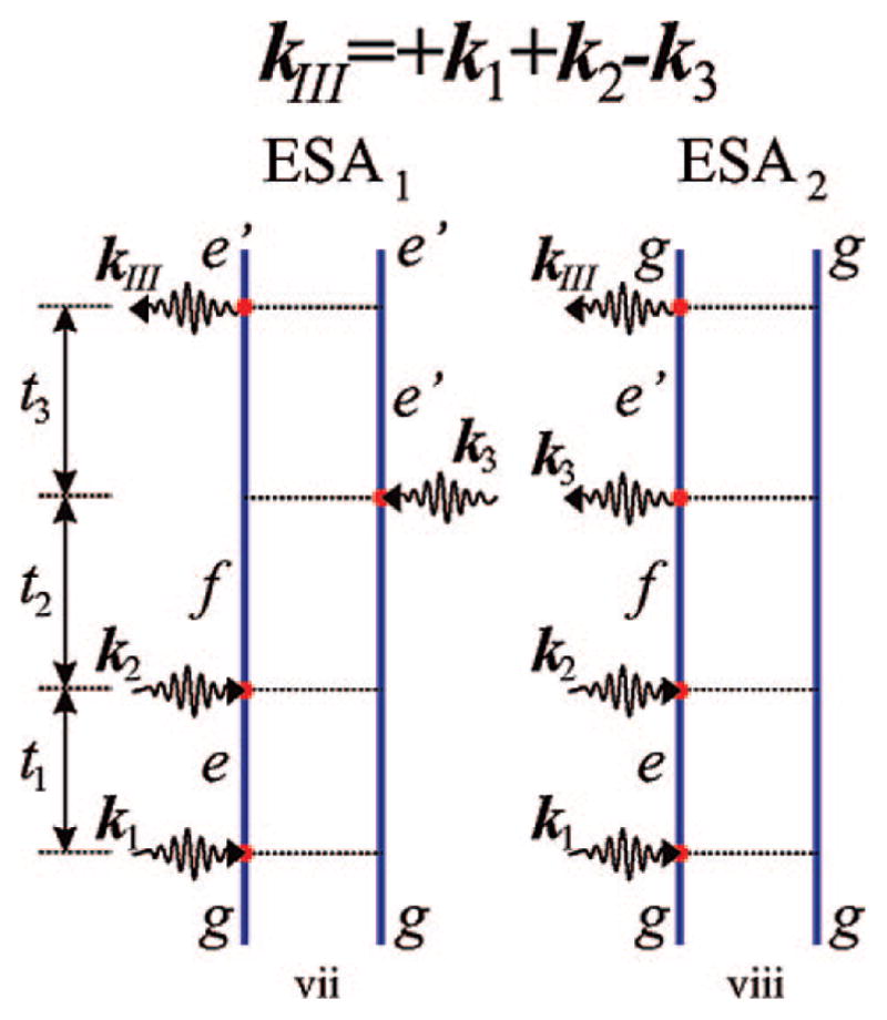
Feynman diagrams as in Figure 5 but for the signal generated in the direction k_III = +k₁ + k₂ − k₃. ESE and GSB do not contribute in this case, and the technique does not show transport. The diagrams are labeled vii and viii for future reference.

The k_I signal is depicted in Figure 4. During t₁, the aggregate density matrix is in an optical coherence with a characteristic frequency given by the energy difference between states e and g, ω_ge. During the second interval (t₂), it is either in the ground state (gg) (ii) or in the singly excited-state manifold (e′e) (i or iii). During the third interval (t₃), it again oscillates with optical frequencies ω_e′g (i and ii) or ω_fe′ (iii).

The various contributions to the signal are denoted ground-state bleaching (GSB), excited-state stimulated emission (ESE), and excited-state absorption (ESA),⁵² as marked in Figure 4. This nomenclature reflects the physical processes during the course of interactions: in the GSB pathway, the system returns to the ground-state during the second interval t₂; thus, the third interaction reflects the reduction of the ground-state population, which reduces (bleaches) the subsequent absorption. In the ESE pathway, during t₂, the system is in the single-excited manifold and the third interaction brings it back to the ground state by stimulated emission. The ESA pathway has the same t₁ and t₂ dynamics as the ESE; however, the third interaction creates a doubly excited state f.

During the intervals between interactions (t₁, t₂, and t₃), the density matrix evolves freely (no field). For instance, in the ESE (Figure 4) diagram, after the first interaction on the right (bra), the system density matrix in the t₁ interval is in the state ρ_ge, and its evolution gives an exp(−iω_get₁) factor, where ω_ge = ε_g − ε_e is the interband frequency. The second interaction from the left with the ket creates the density matrix element ρ_e′e, which then evolves as exp(−iω_e′et₂). After the third interaction (with the bra), the density-matrix element ρ_e′g is created and its evolution is exp(−iω_e′gt₃). The overall contribution of this pathway to the response function is

$$R_i(t_3,t_2,t_1)={\left(\frac{i}{\hslash }\right)}^3\theta (t_1)\theta (t_2)\theta (t_3)\sum _{{ee}^{\prime }}{\mathit{\mu }}_{g{e}^{\prime }}{\mathit{\mu }}_{eg}{\mathit{\mu }}_{e^{\prime }g}{\mathit{\mu }}_{ge}\times exp(-i{\omega }_{ge}{t}_1-i{\omega }_{e^{\prime }e}{t}_2-i{\omega }_{e^{\prime }g}{t}_3-{\gamma }_{ge}{t}_1-{\gamma }_{e^{\prime }e}{t}_2-{\gamma }_{e^{\prime }g}{t}_3),$$ (23)

where the Heavyside step function, θ(t), ensures causality (the response only depends on the fields at earlier times), and we have added the phenomenological dephasing rate γ_ab for the ab coherence.

Similar to the three contributions to the k_I technique shown in Figure 4, k_II has three contributions (Figure 5) and k_III has two contributions (Figure 6). In the next section, we provide closed expressions for all techniques by extending this model to include exciton transport. The expressions corresponding to the diagrams shown in Figures 4–6 may be obtained from eqs 32–39 by setting the population relaxation matrix to unity, ${\mathbb{G}}_{e_2{e}_2,e_1{e}_1}^{(N)}(t_2)=\theta (t_2){\delta }_{e_2{e}_1}$.

Figure 5.

Feynman diagrams as in Figure 4 but for the signal generated in the direction k_II = + k₁ − k₂ + k₃. Population diagrams are labeled iva, v, and via, and the coherence diagrams are labeled ivb and vib.

4. Optical Response of Excitons with Transport; The Lindblad Master Equation

The time evolution of closed quantum systems can be expanded in eigenstates that evolve independently by simply acquiring exp(−iε_jt) phase factors. Open systems (i.e., systems coupled to a bath) undergo various types of relaxation and transport processes. These are commonly described by the evolution of the reduced density matrix of the system, where the bath variables have been projected out.^111,118,119

The dynamics of the reduced density matrix may be described by a quantum master equation (QME). Its general form may be obtained directly from the quantum mechanical analogue of the classical Langevin equations of motion for open systems.¹¹¹ The derivation starts by phenomenologically adding fluctuation and dissipation terms to the Schrödinger equation. This yields the Schrödinger–Langevin equation,

$$\stackrel{.}{\psi }=-\frac{i}{\hslash }\widehat{H}\psi -\frac{1}{2}\sum _{\alpha }{\widehat{V}}_{\alpha }^{†}{\widehat{V}}_{\alpha }\psi +\sum _{\alpha }{\xi }_{\alpha }(t){\widehat{V}}_{\alpha }\psi ,$$ (24)

where ψ is the wave function of the open system, V̂ is an arbitrary set of system operators (independent of ξ) that describe its coupling with the bath, and ξ_α(t) are white noise variables with zero mean, 〈ξ_α(t) 〉= 0, and short correlation time, $\langle {\xi }_{\alpha }(t){\xi }_{\beta }^{\ast }(t^{\prime })\rangle ={\delta }_{\alpha ,\beta }\delta (t-t^{\prime })$. The form of eq 24 guarantees conservation of the norm of the wave function when averaged over the noise.¹¹¹

The QME that corresponds to this Schrödinger–Langevin equation is known as the Lindblad equation.^120–122

$$\stackrel{.}{\widehat{\rho }}=-\frac{i}{\hslash }[\widehat{H},\widehat{\rho }]+\sum _{\alpha }\left({\widehat{V}}_{\alpha }\widehat{\rho }{\widehat{V}}_{\alpha }^{†}-\frac{1}{2}{\widehat{V}}_{\alpha }^{†}{\widehat{V}}_{\alpha }\widehat{\rho }-\frac{1}{2}\widehat{\rho }{\widehat{V}}_{\alpha }^{†}{\widehat{V}}_{\alpha }\right).$$ (25)

It is derived from the Liouville equation for ρ̂(t) ≡ | ψ(t) 〉 〈 (t)| using eq 24 followed by averaging over the noise variables. This equation may be also derived from firmer foundations that show how it preserves all essential properties of the density matrix: it is hermitian with time-independent trace (Tr(ρ̂) ≡ 1) and positive definite.¹¹¹ It will be shown in section 8 that the microscopic Redfield theory in the secular approximation can be recovered by a specific choice of V̂_α. The secular Redfield equations decouple the populations (diagonal elements of ρ̂ in the eigenstate basis) from the coherences (off-diagonal elements). The populations then satisfy the Pauli master equation:^109,111

$$\frac{\text{d}}{\text{d}t}{\rho }_{ee}(t)=-\sum _{e^{\prime }}{K}_{ee,e^{\prime }{e}^{\prime }}{\rho }_{e^{\prime }{e}^{\prime }}(t).$$ (26)

Here, K_{ee, e′e′} is the population transfer rate from state e′ into e. This is an ℕ × ℕ matrix with two pairs of identical indices (ee), (e′e′). In eq 26, the diagonal elements, e = e′, K_{ee, ee} are positive, whereas the off-diagonal elements, e ≠ e′, K_ee, _e′e′ are negative. The rate matrix satisfies Σ_eK_{ee, e′e′} = 0 (probability conservation) and detailed-balance K_{e2e2, e1e1}/K_{e1e1, e2e2} = exp(−ℏω_e2e1/(k_BT)); here, k_B is the Boltzmann constant and T is the temperature. These conditions are sufficient for the system to reach thermal equilibrium at long times.¹¹¹

The evolution of diagonal density-matrix elements is described by the population Green’s function, ${\rho }_{e^{\prime }{e}^{\prime }}(t)={\sum }_e{\mathbb{G}}_{e^{\prime }{e}^{\prime },ee}^{(N)}(t){\rho }_{ee}(0)$, which is the probability of the transition from state e into e′ during time t. The formal solution of the Pauli master equation, eq 26, is given by

$${\mathbb{G}}_{e^{\prime }{e}^{\prime },ee}^{(N)}(t)={[exp(-Kt)]}_{e^{\prime }{e}^{\prime },ee}\equiv \sum _p{\mathit{\chi }}_{e^{\prime }p}^{(\text{R})}{D}_{pp}^{-1}exp(-{\lambda }_{p}t){\mathit{\chi }}_{pe}^{(\text{L})},$$ (27)

where λ_p is the pth eigenvalue of the left- and right-eigen equations ${\sum }_{e^{\prime }}{K}_{ee,e^{\prime }e}{\mathit{\chi }}_{e^{\prime }p}^{(\text{R})}={\lambda }_p{\mathit{\chi }}_{ep}^{(\text{R})}$ and ${\sum }_{e^{\prime }}{K}_{e^{\prime }{e}^{\prime },ee}{\mathit{\chi }}_{p{e}^{\prime }}^{(\text{L})}={\lambda }_p{\mathit{\chi }}_{pe}^{(\text{L})}$. χ^(L) χ ^(R) are matrices made out of the left (right) eigenvectors, and D = χ^(L) χ ^(R) is a diagonal matrix. The eigenvectors are organized as columns of χ ^(R) and rows of χ ^(L). These two sets of eigenvectors are different since K_e′e′, ee is not Hermitian, but they share the same eigenvalues λ_p. χ^(L) and χ^(R) can be normalized as ${\sum }_e{\mathit{\chi }}_{p,e}^{(\text{L})}{\mathit{\chi }}_{e,p}^{(\text{R})}=1$ for each p; then χ ^(R) = χ ^(L)−1 and D is the unitary matrix.

In the secular Redfield equation, the off-diagonal elements satisfy

$$\frac{\text{d}}{\text{d}t}{\rho }_{e^{\prime }e}(t)=[-i{\omega }_{e^{\prime }e}-{\gamma }_{e^{\prime }e}^{(N)}]{\rho }_{e^{\prime }e}(t),e\ne e^{\prime }.$$ (28)

Its solution is ${\rho }_{e^{\prime }e}(t)=exp(-i{\omega }_{e^{\prime }e}t-{\gamma }_{e^{\prime }e}^{(N)}t)$, where

$${\gamma }_{e^{\prime }e}^{(N)}=\frac{1}{2}(K_{ee,ee}+K_{e^{\prime }{e}^{\prime },e^{\prime }{e}^{\prime }})+{\widehat{\gamma }}_{e,e^{\prime }},$$ (29)

The first two terms represent population relaxation, and γ̂_e,e′ is the pure-dephasing rate. For a compact representation of the response functions, we shall combine the diagonal (eq 26) and off-diagonal (eq 28) blocks into a single tetradic Green’s function representing both coherence and population relaxation:

$${\rho }_{e_4{e}_3}(t)=\sum _{e_2{e}_1}{\mathbb{G}}_{e_4{e}_3,e_2{e}_1}^{(N)}(t){\rho }_{e_2{e}_1}(0).$$ (30)

Comparison of eq 30 with eqs 27 and 28 gives

$${\mathbb{G}}_{e_4{e}_3,e_2{e}_1}^{(N)}(t)={\delta }_{e_4{e}_3}{\delta }_{e_2{e}_1}\theta (t){[exp(-Kt)]}_{e_4{e}_4,e_2{e}_2}+(1-{\delta }_{e_4{e}_3}){\delta }_{e_4{e}_2}{\delta }_{e_3{e}_1}\theta (t)exp[-i{\omega }_{e_4{e}_3}t-{\gamma }_{e_4{e}_3}^{(N)}t].$$ (31)

This equation will be derived microscopically and further extended in section 8.

For the k_I and k_II techniques, populations are generated during the second time interval t₂ in the ESA and ESE diagrams of Figures 4 and 5 when e = e′ (GSB includes ground-state population during t₂; since our model contains a single ground state, no population relaxation occurs in the ground state). Population created in state e′ can relax to e during t₂ according to eq 26. Coherences decay according to eq 28.

By including this relaxation model, we obtain the following sum over states (SOS) expression for the response function for the k_I technique (Figures 4 and 7),

Figure 7.

Feynman diagrams for the k_I and k_II signals, which extend diagrams ia, iiia and iva, via of Figures 4 and 5 by including population transport.

$$R_{{\mathit{k}}_{\text{I}},\text{i}}^{(\text{SOS})}(t_3,t_2,t_1)={\left(\frac{i}{\hslash }\right)}^3\theta (t_1)\theta (t_2)\theta (t_3)\sum _{e_4{e}_3{e}_2{e}_1}{\mathit{\mu }}_{g{e}_4}{\mathit{\mu }}_{e_{3}g}{\mathit{\mu }}_{e_{2}g}{\mathit{\mu }}_{g{e}_1}\times exp(-i{\xi }_{e_{4}g}{t}_3-i{\xi }_{g{e}_1}{t}_1){\mathbb{G}}_{e_4{e}_3,e_2{e}_1}^{(N)}(t_2),$$ (32)

$$R_{{\mathit{k}}_{\text{I}},\text{ii}}^{(\text{SOS})}(t_3,t_2,t_1)={\left(\frac{i}{\hslash }\right)}^3\theta (t_1)\theta (t_2)\theta (t_3)\sum _{e_4,e_1}{\mathit{\mu }}_{g{e}_4}{\mathit{\mu }}_{e_{4}g}{\mathit{\mu }}_{e_{1}g}{\mathit{\mu }}_{g{e}_1}\times exp(-i{\xi }_{e_{4}g}{t}_3-i{\xi }_{g{e}_1}{t}_1),$$ (33)

$$R_{{\mathit{k}}_{\text{I}},\text{iii}}^{(\text{SOS})}(t_3,t_2,t_1)=-{\left(\frac{i}{\hslash }\right)}^3\theta (t_1)\theta (t_2)\theta (t_3)\sum _{f{e}_4{e}_3{e}_2{e}_1}{\mathit{\mu }}_{e_{3}f}{\mathit{\mu }}_{f{e}_4}{\mathit{\mu }}_{e_{2}g}{\mathit{\mu }}_{g{e}_1}\times exp(-i{\xi }_{f{e}_3}{t}_3-i{\xi }_{g{e}_1}{t}_1){\mathbb{G}}_{e_4{e}_3,e_2{e}_1}^{(N)}(t_2),$$ (34)

where we have introduced the complex frequencies ξ_ab ≡ ω_ab − iγ_ab. Note that we do not include population relaxation between the excited-state manifold and the ground state; this would change (t₂) and would influence the GSB t₂ dependence.⁵²

The oscillation frequencies during t₁ and t₃ have opposite sense. For a two-level system (g and e), the frequency factors cancel out at t₁ = t₃. This eliminates inhomogeneous broadening and gives rise to the photon-echo signal,^70,123 which has been used for studying dephasing of coherent dynamics in molecules and molecular complexes.^124,125 For multilevel systems (with a band of e states), this cancelation will occur only for the diagonal e = e′ contributions, in the ESE and GSB pathways during t₂ when transport is neglected.

The diagrams shown in Figure 7 extend Figures 4 and 5 to include population transfer during t₂, as marked by the pairs of dashed arrows. For e = e′, the diagrams in Figure 7 coincide with Figures 4 and 5.

For the k_II technique, we similarly have (Figures 5 and 7)

$$R_{{\mathit{k}}_{\text{II}},\text{iv}}^{(\text{SOS})}(t_3,t_2,t_1)={\left(\frac{i}{\hslash }\right)}^3\theta (t_1)\theta (t_2)\theta (t_3)\sum _{e_4{e}_3{e}_2{e}_1}{\mathit{\mu }}_{g{e}_4}{\mathit{\mu }}_{e_{3}g}{\mathit{\mu }}_{g{e}_1}{\mathit{\mu }}_{e_{2}g}\times exp(-i{\xi }_{e_{4}g}{t}_3-i{\xi }_{e_{2}g}{t}_1){\mathbb{G}}_{e_4{e}_3,e_2{e}_1}^{(N)}(t_2),$$ (35)

$$R_{{\mathit{k}}_{\text{II}},\text{v}}^{(\text{SOS})}(t_3,t_2,t_1)={\left(\frac{i}{\hslash }\right)}^3\theta (t_1)\theta (t_2)\theta (t_3)\sum _{e_4{e}_2}{\mathit{\mu }}_{g{e}_4}{\mathit{\mu }}_{e_{4}g}{\mathit{\mu }}_{g{e}_2}{\mathit{\mu }}_{e_{2}g}\times exp(-i{\xi }_{e_{4}g}{t}_3-i{\xi }_{e_{2}g}{t}_1),$$ (36)

$$R_{{\mathit{k}}_{\text{II}},\text{vi}}^{(\text{SOS})}(t_3,t_2,t_1)=-{\left(\frac{i}{\hslash }\right)}^3\theta (t_1)\theta (t_2)\theta (t_3)\sum _{f{e}_4{e}_3{e}_2{e}_1}{\mathit{\mu }}_{e_{3}f}{\mathit{\mu }}_{f{e}_4}{\mathit{\mu }}_{g{e}_1}{\mathit{\mu }}_{e_{2}g}\times exp(-i{\xi }_{f{e}_3}{t}_3-i{\xi }_{e_{2}g}{t}_1){\mathbb{G}}_{e_4{e}_3,e_2{e}_1}^{(N)}(t_2).$$ (37)

The two contributions to the k_III (Figure 6) technique are of the ESA type:

$$R_{{\mathit{k}}_{\text{III}},\text{vii}}^{(\text{SOS})}(t_3,t_2,t_1)=-{\left(\frac{i}{\hslash }\right)}^3\theta (t_1)\theta (t_2)\theta (t_3)\sum _{{ee}^{\prime }f}{\mathit{\mu }}_{e^{\prime }f}{\mathit{\mu }}_{g{e}^{\prime }}{\mathit{\mu }}_{fe}{\mathit{\mu }}_{eg}\times exp(-i{\xi }_{f{e}^{\prime }}{t}_3-i{\xi }_{fg}{t}_2-i{\xi }_{eg}{t}_1),$$ (38)

$$R_{{\mathit{k}}_{\text{III}},\text{viii}}^{(\text{SOS})}(t_3,t_2,t_1)={\left(\frac{i}{\hslash }\right)}^3\theta (t_1)\theta (t_2)\theta (t_3)\sum _{{ee}^{\prime }f}{\mathit{\mu }}_{g{e}^{\prime }}{\mathit{\mu }}_{e^{\prime }f}{\mathit{\mu }}_{fe}{\mathit{\mu }}_{eg}\times exp(-i{\xi }_{e^{\prime }g}{t}_3-i{\xi }_{fg}{t}_2-i{\xi }_{eg}{t}_1).$$ (39)

Note that exciton transport only enters k_I and k_II but not k_III where exciton populations are never created.

The present phenomenological model allows an easy calculation of the response functions. Exciton relaxation is described by Markovian rate equations. More elaborate decay patterns that show oscillations and nonexponential correlated dynamics often observed in molecular aggregates^41,48,126 require higher levels of theory that will be presented in the coming sections.

5. Multidimensional Spectroscopy of a Three-Band Model; Heterodyne-Detected Signals

The response functions introduced earlier may be used to calculate the polarization induced by a resonant excitation. The relation between the signal and the induced polarization depends on the detection mode, as described in Appendix B. Heterodyne detection is the most advanced detection method that gives the signal field itself (both amplitude and phase).

The third-order heterodyne-detected signal is given by

$$S_{{\mathit{k}}_s}^{(3)}(T_3,T_2,T_1)={\int }_{-\infty }^{\infty }\text{d}t{\mathit{P}}_{{\mathit{k}}_s}(t){\mathbb{E}}_s^{\ast }(t-{\tau }_s){\text{e}}^{i{\omega }_s(t-{\tau }_s)},$$ (40)

where the signal depends parametrically on the delays between pulses T₃ = τ_s − τ₃, T₂ = τ₃ − τ₂, and T₁ = τ₂ − τ₁. The notation τ ≡ T₁, T ≡ T₂, and t ≡ T₃ is commonly used. Experimentally the signal field is often dispersed in a spectrometer. The entire T₃ dependence is then measured in a single shot rather by scanning the delay between the third pulse and the signal. (t – τ_s) is the local oscillator field envelope used for heterodyne detection. The first three pulses are represented by eq 16, and the third-order polarization P⁽³⁾(t) is given by eq 18.

Multidimensional signals are displayed in the frequency domain by Fourier transforming $S_{{\mathit{k}}_s}^{(3)}(T_3,T_2,T_1)$ with respect to the time intervals between the pulses.

$$S_{{\mathit{k}}_s}^{(3)}({\mathrm{\Omega }}_3,{\mathrm{\Omega }}_2,{\mathrm{\Omega }}_1)={\int }_0^{\infty }\text{d}{T}_3{\int }_0^{\infty }\text{d}{T}_2{\int }_0^{\infty }\text{d}{T}_1{\text{e}}^{i{\mathrm{\Omega }}_3{T}_3+i{\mathrm{\Omega }}_2{T}_2+i{\mathrm{\Omega }}_1{T}_1}{S}_{{\mathit{k}}_s}^{(3)}(T_3,T_2,T_1).$$ (41)

Often, one uses a mixed time-frequency representation by performing double-Fourier transform. This gives, e.g., S(Ω₃, T₂, Ω₁), etc.

Assuming that all four pulses are temporally well-separated, the integrations can be carried out using the response function eqs 32–39.¹²⁷ Neglecting population transport (K_{ee, e′e′} ≡ 0), this gives the following three contributions to the k_I signal (see Figures 4–6),

$$S_{{\mathit{k}}_{\text{I}},\text{i}}^{(\text{SOS})}({\mathrm{\Omega }}_3,{\mathrm{\Omega }}_2,{\mathrm{\Omega }}_1)=-\sum _{{ee}^{\prime }}({\mathit{\mu }}_{e^{\prime }g}^{\ast }·{\mathbb{E}}_s^{\ast }({\omega }_{e^{\prime }g}-{\omega }_s))({\mathit{\mu }}_{eg}·{\mathbb{E}}_3({\omega }_{eg}-{\omega }_3))\times \frac{({\mathit{\mu }}_{e^{\prime }g}·{\mathbb{E}}_2({\omega }_{e^{\prime }g}-{\omega }_2))({\mathit{\mu }}_{eg}^{\ast }·{\mathbb{E}}_1^{\ast }({\omega }_{eg}-{\omega }_1))}{{\hslash }^3({\mathrm{\Omega }}_3-{\xi }_{e^{\prime }g})({\mathrm{\Omega }}_2-{\xi }_{e^{\prime }e})({\mathrm{\Omega }}_1-{\xi }_{ge})},$$ (42)

$$S_{{\mathit{k}}_{\text{I}},\text{ii}}^{(\text{SOS})}({\mathrm{\Omega }}_3,{\mathrm{\Omega }}_2,{\mathrm{\Omega }}_1)=-\sum _{{ee}^{\prime }}({\mathit{\mu }}_{e^{\prime }g}^{\ast }·{\mathbb{E}}_s^{\ast }({\omega }_{e^{\prime }g}-{\omega }_s))({\mathit{\mu }}_{e^{\prime }g}·{\mathbb{E}}_3({\omega }_{e^{\prime }g}-{\omega }_3))\times \frac{({\mathit{\mu }}_{eg}·{\mathbb{E}}_2({\omega }_{eg}-{\omega }_2))({\mathit{\mu }}_{eg}^{\ast }·{\mathbb{E}}_1^{\ast }({\omega }_{eg}-{\omega }_1))}{{\hslash }^3({\mathrm{\Omega }}_3-{\xi }_{e^{\prime }g})({\mathrm{\Omega }}_2-i\eta )({\mathrm{\Omega }}_1-{\xi }_{ge})},$$ (43)

$$S_{{\mathit{k}}_{\text{I}},\text{iii}}^{(\text{SOS})}({\mathrm{\Omega }}_3,{\mathrm{\Omega }}_2,{\mathrm{\Omega }}_1)=\sum _{{\mathit{fee}}^{\prime }}({\mathit{\mu }}_{fe}^{\ast }·{\mathbb{E}}_s^{\ast }({\omega }_{fe}-{\omega }_s))({\mathit{\mu }}_{f{e}^{\prime }}·{\mathbb{E}}_3({\omega }_{f{e}^{\prime }}-{\omega }_3))\times \frac{({\mathit{\mu }}_{e^{\prime }g}·{\mathbb{E}}_2({\omega }_{e^{\prime }g}-{\omega }_2))({\mathit{\mu }}_{eg}^{\ast }·{\mathbb{E}}_1^{\ast }({\omega }_{eg}-{\omega }_1))}{{\hslash }^3({\mathrm{\Omega }}_3-{\xi }_{fe})({\mathrm{\Omega }}_2-{\xi }_{e^{\prime }e})({\mathrm{\Omega }}_1-{\xi }_{ge})},$$ (44)

where e and e′ run over the single-exciton manifold, f runs over the two-exciton states, and η→ +0. ω₁, ω₂, and ω₃ are the carrier frequencies of the first three pulses, and ω_ab and ξ_ab were defined in sections 2 and 4. The spectral pulse envelopes

$$\mathbb{E}(\omega )=\int \text{d}texp(i\omega t)\mathbb{E}(t)$$ (45)

are centered around ω = 0.

For the k_II signal, we similarly obtain

$$S_{{\mathit{k}}_{\text{II}},\text{iv}}^{(\text{SOS})}({\mathrm{\Omega }}_3,{\mathrm{\Omega }}_2,{\mathrm{\Omega }}_1)=-\sum _{{ee}^{\prime }}({\mathit{\mu }}_{eg}^{\ast }·{\mathbb{E}}_s^{\ast }({\omega }_{eg}-{\omega }_s))({\mathit{\mu }}_{e^{\prime }g}·{\mathbb{E}}_3({\omega }_{e^{\prime }g}-{\omega }_3))\times \frac{({\mathit{\mu }}_{e^{\prime }g}^{\ast }·{\mathbb{E}}_2^{\ast }({\omega }_{e^{\prime }g}-{\omega }_2))({\mathit{\mu }}_{eg}·{\mathbb{E}}_1({\omega }_{eg}-{\omega }_1))}{{\hslash }^3({\mathrm{\Omega }}_3-{\xi }_{eg})({\mathrm{\Omega }}_2-{\xi }_{{ee}^{\prime }})({\mathrm{\Omega }}_1-{\xi }_{eg})},$$ (46)

$$S_{{\mathit{k}}_{\text{II}},\text{v}}^{(\text{SOS})}({\mathrm{\Omega }}_3,{\mathrm{\Omega }}_2,{\mathrm{\Omega }}_1)=-\sum _{{ee}^{\prime }}({\mathit{\mu }}_{e^{\prime }g}^{\ast }·{\mathbb{E}}_s^{\ast }({\omega }_{e^{\prime }g}-{\omega }_s))({\mathit{\mu }}_{e^{\prime }g}·{\mathbb{E}}_3({\omega }_{e^{\prime }g}-{\omega }_3))\times \frac{({\mathit{\mu }}_{eg}^{\ast }·{\mathbb{E}}_2^{\ast }({\omega }_{eg}-{\omega }_2))({\mathit{\mu }}_{eg}•{\mathbb{E}}_1({\omega }_{eg}-{\omega }_1))}{{\hslash }^3({\mathrm{\Omega }}_3-{\xi }_{e^{\prime }g})({\mathrm{\Omega }}_2+i\eta )({\mathrm{\Omega }}_1-{\xi }_{eg})},$$ (47)

$$S_{{\mathit{k}}_{\text{II}},\text{vi}}^{(\text{SOS})}({\mathrm{\Omega }}_3,{\mathrm{\Omega }}_2,{\mathrm{\Omega }}_1)=\sum _{{\mathit{fee}}^{\prime }}({\mathit{\mu }}_{f{e}^{\prime }}^{\ast }·{\mathbb{E}}_s^{\ast }({\omega }_{f{e}^{\prime }}-{\omega }_s))({\mathit{\mu }}_{fe}·{\mathbb{E}}_3({\omega }_{fe}-{\omega }_3))\times \frac{({\mathit{\mu }}_{e^{\prime }g}^{\ast }·{\mathbb{E}}_2^{\ast }({\omega }_{e^{\prime }g}-{\omega }_2))({\mathit{\mu }}_{eg}·{\mathbb{E}}_1({\omega }_{eg}-{\omega }_1))}{{\hslash }^3({\mathrm{\Omega }}_3-{\xi }_{f{e}^{\prime }})({\mathrm{\Omega }}_2-{\xi }_{{ee}^{\prime }})({\mathrm{\Omega }}_1-{\xi }_{eg})},$$ (48)

Finally, the k_III signal is given by

$$S_{{\mathit{k}}_{\text{III}},\text{vii}}^{(\text{SOS})}({\mathrm{\Omega }}_3,{\mathrm{\Omega }}_2,{\mathrm{\Omega }}_1)=\sum _{{\mathit{fee}}^{\prime }}({\mathit{\mu }}_{f{e}^{\prime }}^{\ast }·{\mathbb{E}}_s^{\ast }({\omega }_{f{e}^{\prime }}-{\omega }_s))({\mathit{\mu }}_{e^{\prime }g}^{\ast }·{\mathbb{E}}_s^{\ast }({\omega }_{e^{\prime }g}-{\omega }_3))\times \frac{({\mathit{\mu }}_{fe}·{\mathbb{E}}_2({\omega }_{fe}-{\omega }_2))({\mathit{\mu }}_{eg}·{\mathbb{E}}_1({\omega }_{eg}-{\omega }_1))}{{\hslash }^3({\mathrm{\Omega }}_3-{\xi }_{f{e}^{\prime }})({\mathrm{\Omega }}_2-{\xi }_{fg})({\mathrm{\Omega }}_1-{\xi }_{eg})},$$ (49)

and

$$S_{{\mathit{k}}_{\text{III}},\text{viii}}^{(\text{SOS})}({\mathrm{\Omega }}_3,{\mathrm{\Omega }}_2,{\mathrm{\Omega }}_1)=-\sum _{e^{\prime }fe}({\mathit{\mu }}_{e^{\prime }g}^{\ast }·{\mathbb{E}}_s^{\ast }({\omega }_{e^{\prime }g}-{\omega }_s))({\mathit{\mu }}_{f{e}^{\prime }}^{\ast }·{\mathbb{E}}_3^{\ast }({\omega }_{f{e}^{\prime }}-{\omega }_3))\times \frac{({\mathit{\mu }}_{fe}·{\mathbb{E}}_2({\omega }_{fe}-{\omega }_2))({\mathit{\mu }}_{eg}·{\mathbb{E}}_1({\omega }_{eg}-{\omega }_1))}{{\hslash }^3({\mathrm{\Omega }}_3-{\xi }_{e^{\prime }g})({\mathrm{\Omega }}_2-{\xi }_{fg})({\mathrm{\Omega }}_1-{\xi }_{eg})}.$$ (50)

Note that resonances occur at both positive and negative Ω_j.

Population relaxation may be added, as done in eqs 32–39. However, the Ω₂ dependence is then more complicated, and it is usually preferable to display the signal S(Ω₃, T₂, Ω₁) in the time domain as a function of T₂.

Equations 42–50 show how the pulse envelopes select the possible transitions allowed by their bandwidths. The pulse envelopes serve as frequency filters, removing all transitions falling outside the pulse bandwidth. If the pulse bandwidth is larger than the exciton bandwidth, we can set &(ω) = 1. This impulsive signal then coincides with the response function.

This concludes the phenomenological supermolecule description of multidimensional signals in terms of the global eigenstates. In the next section, we present the alternative, quasiparticle, picture. Numerical applications of both approaches will be presented in the following sections.

6. Quasiparticle Representation of the Optical Response; The Nonlinear-Exciton Equations (NEE)

The calculation of double-exciton states requires the computationally expensive diagonalization of an × matrix, where = ℕ (ℕ ± 1)/2 is the number of double-exciton states, and ℕ is the number of molecules. The quasiparticle picture avoids the explicit calculation of the two-exciton states making it more tractable in large aggregates.^{68,79,102,104,106–108,128} This picture naturally emerges out of equations of motion for exciton variables, the NEE, that were derived and gradually developed at different levels.^79,107,108 Spano and Mukamel had shown how theories of optical susceptibilities in the frequency domain based on the local mean-field approximation (MFA) can be extended by adding two-exciton variables to properly account for two-exciton resonances.^102,128 The nonlinear response is then attributed to exciton–exciton scattering.^104,105 The formalism was subsequently extended to molecular aggregates made of three-level molecules and to semiconductors.^68,114 Additional relevant variables have been introduced to account for exciton relaxation due to coupling with phonons.⁶⁸ The phonon degrees of freedom are formally eliminated; they only enter through the relaxation rates. This results in the Redfield equations for the reduced exciton density matrix.

By solving the NEE, we obtain closed Green’s function expressions for the optical response that maintain the complete bookkeeping of time ordering. Applications of this approach were made to J-aggregates,¹⁰³ pump–probe, photonechoes, and other four-wave mixing techniques of light-harvesting antenna complexes.^78,130,131

We first introduce the microscopic exciton model for an aggregate made out of ℕ three-level chromophores. The special case of two-level chromophores is treated in Appendix C. Electronic excitations are expressed using the basis set of the electronic eigenstates of each chromophore: these are the ground state ${\phi }_m^{(g)}$, the single-excited state ${\phi }_m^{(e)}$, and the double-excited state ${\phi }_m^{(f)}$. In the Heitler–London approximation,¹⁷ the aggregate ground state is given by a direct product of the ground states of all chromophores,

$${\mathrm{\Phi }}_g={\prod }_m^{\mathbb{N}}{\phi }_m^{(g)}.$$ (51)

A single-excited-state basis is constructed by moving one of the chromophores into its excited state,

$${\mathrm{\Phi }}_{e_m}={\phi }_m^{(e)}{\prod }_k^{k\ne m}{\phi }_k^{(g)}.$$ (52)

Double-excitations are obtained either when one of the chromophores is doubly excited

$${\mathrm{\Phi }}_{f_{mm}}={\phi }_m^{(f)}{\prod }_k^{k\ne m}{\phi }_k^{(g)}$$ (53)

or when two chromophores are singly excited:

$${\mathrm{\Phi }}_{f_{mn}}={\phi }_m^{(e)}{\phi }_n^{(e)}{\prod }_k^{k\ne m,k\ne n}{\phi }_k^{(g)}.$$ (54)

Overall, our model has ℕ singly excited states, and = ℕ( ℕ + 1)/2 doubly-excited states.

We next introduce an exciton-creation operator on molecule m:¹³¹

$${\widehat{B}}_m^{†}=\mid {\phi }_m^{(e)}\rangle \langle {\phi }_m^{(g)}\mid +\sqrt{2}\mid {\phi }_m^{(f)}\rangle \langle {\phi }_m^{(e)}\mid .$$ (55)

These operators have the following properties: single-exciton states are created from the ground state ${\mathrm{\Phi }}_{e_m}={\widehat{B}}_m^{†}{\mathrm{\Phi }}_g$, and double-excitons are obtained either by creating two excitations on different molecules, ${\mathrm{\Phi }}_{f_{mn};m\ne n}={\widehat{B}}_m^{†}{\widehat{B}}_n^{†}{\mathrm{\Phi }}_g$, or on the same molecule, ${\mathrm{\Phi }}_{f_{mm}}=2^{-1/2}{\widehat{B}}_m^{†2}{\mathrm{\Phi }}_g$ (the √2 factor is introduced to resemble bosonic exciton properties ( ${\widehat{B}}^{†}\mid n-1\rangle =\sqrt{n}\mid n\rangle$) within the single- and double-exciton space).

The Hermitian-conjugate, annihilation, operator will be denoted B̂_m. Operators corresponding to different chromophores commute. The commutation relations of these operators are (see Appendix C)

$$[{\widehat{B}}_n,{\widehat{B}}_m^{†}]={\delta }_{mn}\left(1-\frac{3}{2}{\widehat{B}}_m^{†2}{\widehat{B}}_m^2\right).$$ (56)

Only these operators are required to describe the linear and the third-order optical signals, which involve up to double-exciton states. Higher, e.g., triple, excitations, B̂^†B̂^†B̂^†Φ_g, will not be considered.

We assume the following model Hamiltonian written in a normally ordered form (i.e., all B̂^† are to the left of B̂)⁶⁸

$${\widehat{H}}_0=\hslash \sum _m{\epsilon }_m{\widehat{B}}_m^{†}{\widehat{B}}_m+\hslash \sum _{mn}^{m\ne n}{J}_{mn}{\widehat{B}}_m^{†}{\widehat{B}}_n+\hslash \sum _{\mathit{mnkl}}{U}_{mn,kl}{\widehat{B}}_m^{†}{\widehat{B}}_n^{†}{\widehat{B}}_k{\widehat{B}}_l,$$ (57)

where ℏε_n is the single-excitation energy of molecule n and quadratic coupling ℏJ_mn is responsible for resonant exciton hopping.^132–134 The quartic couplings ℏU_mn,kl represent various types of anharmonicities that only affect the two-exciton (and higher) manifolds. Terms that do not conserve the number of excitons, such as ${\widehat{B}}_m^{†}$ and ${\widehat{B}}_m^{†2}$, have been neglected in this Hamiltonian (a more general Hamiltonian is discussed in ref 135).

A simplified form of eq 57,

$${\widehat{H}}_0=\hslash \sum _m{\epsilon }_m{\widehat{B}}_m^{†}{\widehat{B}}_m+\hslash \sum _{mn}^{m\ne n}{J}_{mn}{\widehat{B}}_m^{†}{\widehat{B}}_n+\hslash \sum _m\frac{{\mathrm{\Delta }}_m}{2}{\widehat{B}}_m^{†}{\widehat{B}}_m^{†}{\widehat{B}}_m{\widehat{B}}_m+\hslash \sum _{mn}^{m\ne n}\frac{{\mathbb{K}}_{mn}}{2}{\widehat{B}}_m^{†}{\widehat{B}}_n^{†}{\widehat{B}}_m{\widehat{B}}_n$$ (58)

captures the essential physical processes. The diagonal term Δ_m = 2U_mm,mm modifies the energy of two excitations on the same site: 〈Φ_fmm|Ĥ₀|Φ_fmm〉/ℏ = 2ε_m + Δ_m. Two-level chromophores can be described by setting Δ_m → ∞. This prevents two excitations from residing on the same site. The couplings /4 = U_{mn, mn} ≡U_{mn, nm} shift the two-exciton energies with respect to the noninteracting excitons 〈Φ_fmn|Ĥ₀|Φ_fmn〉/ℏ = ε_m + ε_n + . They can be either repulsive, > 0, or attractive, < 0.

We further assume the following form for the dipole operator where each interaction with the field can create or annihilate a single exciton:

$$\widehat{\mathit{\mu }}=\sum _m[{\mathit{\mu }}_m{\widehat{B}}_m^{†}+{\mathit{\mu }}_m^{(2)}{\widehat{B}}_m^{†2}{\widehat{B}}_m+h.c].$$ (59)

Here, h.c denotes the Hermitian conjugate. The transition dipole 〈Φ_g|μ̂ |Φ_em〉 = μ_m gives the transition between the ground and a single-excited state and $\langle {\mathrm{\Phi }}_{e_m}\mid \widehat{\mathit{\mu }}\mid {\mathrm{\Phi }}_{f_{mm}}\rangle =\sqrt{2}({\mathit{\mu }}_m+{\mathit{\mu }}_m^{(2)})$ is the transition between a single- and a double-excited state. Within the RWA, the coupling with the field (eq 3) is given by

$${\widehat{H}}^{\prime }(t)=\hslash \sum _{m,j}({\mu }_{m,j}^{-}(t){\widehat{B}}_m^{†}+{\mu }_{m,j}^{+}(t){\widehat{B}}_m+{\mu }_{m,j}^{(2)-}(t){\widehat{B}}_m^{†2}{\widehat{B}}_m+{\mu }_{m,j}^{(2)+}(t){\widehat{B}}_m^{†}{\widehat{B}}_m^2),$$ (60)

where

$${\mu }_{m,j}^{-}(t)=-{\hslash }^{-1}{\mathit{\mu }}_m·{\mathbb{E}}_j(t-{\tau }_j)exp(i{\mathit{k}}_j\mathit{r}-i{\omega }_{j}t)$$ (61)

and

$${\mu }_{m,j}^{(2)-}(t)=-{\hslash }^{-1}{\mathit{\mu }}_m^{(2)}·{\mathbb{E}}_j(t-{\tau }_j)exp(i{\mathit{k}}_j\mathit{r}-i{\omega }_{j}t)$$ (62)

are the time-dependent transition amplitudes with μ⁻ ≡ (μ⁺)*: μ⁻ annihilates the photon and, thus, is conjugated to the creation of exciton, while μ⁺ creates the photon accompanied by annihilation of the exciton. The total Hamiltonian is given by eq 1 together with eqs 57 and 60.

The exciton dynamics will be calculated starting with the Heisenberg equations of motion

$$i\hslash \frac{\text{d}\widehat{A}}{\text{d}t}=[\widehat{A},\widehat{H}].$$ (63)

Taking  = B̂_m and  = B̂_mB̂_n gives

$$i\frac{\text{d}}{\text{d}t}{\widehat{B}}_m=\sum _{m^{\prime }}{h}_{m{m}^{\prime }}{\widehat{B}}_{m^{\prime }}+\sum _{m^{\prime }kl}{V}_{m{m}^{\prime },kl}{\widehat{B}}_{m^{\prime }}^{†}{\widehat{B}}_k{\widehat{B}}_l+\sum _j[{\mu }_{m,j}^{-}+2{\mu }_{m,j}^{(2)-}{\widehat{B}}_m^{†}{\widehat{B}}_m+{\mu }_{m,j}^{(2)+}{\widehat{B}}_m{\widehat{B}}_m],$$ (64)

$$i\frac{\text{d}}{\text{d}t}{\widehat{B}}_m{\widehat{B}}_n=\sum _{m^{\prime }{n}^{\prime }}{h}_{mn,m^{\prime }{n}^{\prime }}^{(Y)}{\widehat{B}}_{m^{\prime }}{\widehat{B}}_{n^{\prime }}+\sum _{m^{\prime }kl}[V_{m{m}^{\prime },kl}{\widehat{B}}_{m^{\prime }}^{†}{\widehat{B}}_k{\widehat{B}}_l{\widehat{B}}_n+V_{n{m}^{\prime },kl}{\widehat{B}}_{n^{\prime }}^{†}{\widehat{B}}_k{\widehat{B}}_l{\widehat{B}}_m]+\sum _j[{\mu }_{m,j}^{-}{\widehat{B}}_n+{\mu }_{n,j}^{-}{\widehat{B}}_m+2{\delta }_{mn}{\mu }_{m,j}^{(2)-}{\widehat{B}}_m+2{\mu }_{n,j}^{(2)-}{\widehat{B}}_n^{†}{\widehat{B}}_n{\widehat{B}}_m+2{\mu }_{m,j}^{(2)-}{\widehat{B}}_m^{†}{\widehat{B}}_m{\widehat{B}}_n+2{\mu }_{n,j}^{(2)+}{\widehat{B}}_n{\widehat{B}}_n{\widehat{B}}_m],$$ (65)

with

$$h_{mn}=J_{mn}(1-{\delta }_{mn})+{\delta }_{mn}{\epsilon }_m,$$ (66)

$$h_{mn,m^{\prime }{n}^{\prime }}^{(Y)}=h_{m{m}^{\prime }}{\delta }_{n{n}^{\prime }}+h_{n{n}^{\prime }}{\delta }_{m{m}^{\prime }}+V_{mn,m^{\prime }{n}^{\prime }}$$ (67)

and V_mn,kl = U_mn,kl + U_nm,kl. These are the first two members of an infinite hierarchy of coupled equations.

Different-order contributions in the field can be easily sorted out in these equations since interactions with the field change the number of excitons one at a time. Thus, μ is first order, B̂ is first order and higher, B̂^†B̂B̂ and ${\mathit{\mu }}^{(2)}{B}_m^{†}{\widehat{B}}_m$ are third order and higher, and B̂^†B̂B̂B̂ is at least fourth order, etc.

When the system is in a pure state, it can be described by a wave function (the expansion $\mathrm{\Phi }={\sum }_m{c}_m{\widehat{B}}_m^{†}\mid 0\rangle +C_{mn}{\widehat{B}}_m^{†}{\widehat{B}}_n^{†}\mid 0\rangle$ is sufficient to represent the third-order response), and we have $\langle {\widehat{B}}_m^{†}{\widehat{B}}_n\rangle =\langle {\widehat{B}}_m^{†}\rangle \langle {\widehat{B}}_n\rangle$. We can further factorize $\langle {\widehat{B}}_m^{†}{\widehat{B}}_n{\widehat{B}}_k\rangle =B_m^{\ast }{Y}_{nk}$ where we used B = 〈B〉 and Y_mn = 〈B̂_mB̂_n〉. Taking expectation value of both sides of eqs 64 and 65, we obtain the NEE to third order in the field¹⁰⁷

$$i\frac{\text{d}}{\text{d}t}{B}_m=\sum _{m^{\prime }}{h}_{m{m}^{\prime }}{B}_{m^{\prime }}+\sum _{m^{\prime }kl}{V}_{m{m}^{\prime },kl}{B}_{m^{\prime }}^{\ast }{Y}_{kl}+\sum _j[{\mu }_{m,j}^{-}+2{\mu }_{m,j}^{(2)-}{B}_m^{\ast }{B}_m+{\mu }_{m,j}^{(2)+}{Y}_{mm}],$$ (68)

$$i\frac{\text{d}}{\text{d}t}{Y}_{mn}=\sum _{m^{\prime }{n}^{\prime }}{h}_{mn,m^{\prime }{n}^{\prime }}^{(Y)}{Y}_{m^{\prime }{n}^{\prime }}+\sum _j[{\mu }_{m,j}^{-}{B}_n+{\mu }_{n,j}^{-}{B}_m+2{\delta }_{mn}{\mu }_{m,j}^{(2)-}{B}_m].$$ (69)

Quartic products B̂^†2B̂² contribute only to fourth and higher orders in the fields and were neglected. Within this space of relevant states, the exciton commutation relation, eq 56, can be, therefore, replaced by the boson commutation relation,

$${[{\widehat{B}}_m,{\widehat{B}}_n^{†}]}_{\text{boson}}={\delta }_{mn},$$ (70)

which we use in the following derivations. Equation 70 allows the creation of triple- and higher-exciton states on each chromophore; however, these lie outside of the physical space of states relevant for third-order spectroscopy. Exact bosonization procedures can be performed for arbitrary models of nonbosonic truncated oscillators^99,136,137 as well as fermions.^107,138,139 We review the bosonization of two-level molecules in Appendix C. The same ideas can be applied to multilevel molecules (truncated oscillators).

Different levels of approximation will be introduced for truncating the hierarchy of eqs 64 and 65. The simplest, mean-field approximation (MFA), which is equivalent to the Hartree–Fock approximation in many-electron problems¹¹⁴ uses the full factorization of all normally ordered products 〈B̂B̂〉 = 〈B̂〉〈B̂〉 and 〈B̂^†B̂〉 = 〈B̂^†〉〈B̂〉, 〈B̂^†B̂B̂〉 = 〈B̂^†〉〈B̂〉〈B̂〉.^102,128 The excitons are treated as noninteracting quasiparticles, each moving in the mean field created by the others. Equation 64 is then closed, and the other equations become redundant.¹⁰³ A higher-level approximation factorizes all daggered and undaggered variables 〈B̂^†B̂〉 = 〈B̂^†〉〈B̂〉and 〈B̂^†B̂B̂〉 = 〈B̂^†〉〈B̂B̂〉, while retaining the 〈B̂B̂〉 variables.^79,104,105 This coherent exciton dynamics (CED) takes into account two-particle statistics but neglects transport. Equations 68 and 69 then form a complete closed set. Another possible factorization 〈B̂^†B̂B̂〉 = 〈B̂^†B̂〉〈B̂〉 neglects double-exciton statistical properties, while maintaining transport. This level of theory is equivalent to the Semiconductor Bloch equations (SBE) with dephasing, used for Wannier excitons.¹¹⁴ The response functions predicted by these various levels of approximation will be discussed in the coming sections.

7. Coherent Nonlinear Optical Response of Quasiparticles in the Molecular Basis

The response functions, eqs 14 and 18, connect the induced polarization to the incoming laser electric fields. The third-order signals can be calculated using the Green’s function solution of the equation hierarchy, eqs 64 and 65 (eqs 68 and 69 as a special case). The induced polarization is defined as the expectation value of the dipole operator (eq 59).

7.1. Linear Response

In the linear regime, we get

$${\mathit{P}}^{(1)}(t)=\sum _m{\mathit{\mu }}_m^{\ast }{B}_m^{(1)}(t)+c.c.$$ (71)

Single-exciton dynamics when the field is switched off is described by

$$i\frac{\text{d}}{\text{d}t}{B}_m^{(1)}=\sum _{m^{\prime }}{h}_{m{m}^{\prime }}{B}_{m^{\prime }}^{(1)},$$ (72)

obtained from eq 68 with Y ≡0. Propagation of excitons is described by a single-exciton Green’s function,

$$\frac{\text{d}}{\text{d}t}{G}_{mn}=-i\sum _{m^{\prime }}{h}_{m{m}^{\prime }}{G}_{m^{\prime }n}+\delta (t){\delta }_{mn},$$ (73)

whose solution is G(t) = θ(t) exp(−iht), where h is the matrix with elements h_mn. The solution of eq 72 is given by $B_m^{(1)}(t)=G_{mn}(t)B_n^{(1)}(0)$.

The first-order terms in the NEE equations are obtained from

$$i\frac{\text{d}}{\text{d}t}{B}_m^{(1)}=\sum _{m^{\prime }}{h}_{m{m}^{\prime }}{B}_{m^{\prime }}^{(1)}+\sum _j{\mu }_{m,j}^{-}.$$ (74)

Substituting the Green’s function solution of eq 74,

$$B_m^{(1)}(t)=-i{\int }_{-\infty }^t\text{d}\tau \sum _{n,j}{G}_{mn}(t-\tau ){\mu }_{n,j}^{-}(\tau )$$ (75)

into eq 71, and using eq 11, we get the linear response function:

$$R^{(1)}(t)={\left(\frac{i}{\hslash }\right)}^1\sum _{mn}{\mathit{\mu }}_m^{\ast }{\mathit{\mu }}_n{G}_{mn}(t)+c.c.$$ (76)

Linear response techniques are surveyed in Appendix A.

7.2. Third-Order Response

The third-order induced polarization is

$${\mathit{P}}^{(3)}(t)=\sum _m{\mathit{\mu }}_m^{\ast }{\langle {\widehat{B}}_m\rangle }^{(3)}+{\mathit{\mu }}_m^{(2)\ast }{\langle {\widehat{B}}_m^{†}{\widehat{B}}_m{\widehat{B}}_m\rangle }^{(3)}+c.c.$$ (77)

Below, we present two levels of approximation for the k_I, k_II, and k_III techniques: the MFA and the coherent exciton dynamics (CED) limit.

7.2.1. Mean-Field Approximation

At this level of theory, we make the factorizations 〈B̂B̂〉 = 〈B̂〉〈B̂〉. Equation 68 then becomes

$$i\frac{\text{d}}{\text{d}t}{B}_m=\sum _{m^{\prime }}{h}_{m{m}^{\prime }}{B}_{m^{\prime }}+\sum _{m^{\prime }kl}{V}_{m{m}^{\prime },kl}{B}_{m^{\prime }}^{\ast }{B}_k{B}_l+\sum _j{\mu }_{m,j}^{-}+2{\mu }_{m,j}^{(2)-}{B}_m^{\ast }{B}_m+{\mu }_{m,j}^{(2)+}{B}_m{B}_m$$ (78)

and the polarization (eq 77) reduces to

$${\mathit{P}}^{(3)}(r,t)=\sum _m[{\mathit{\mu }}_m^{\ast }{B}_m^{(3)}(t)+{\mathit{\mu }}_m^{(2)\ast }{B}_m^{(1)\ast }(t)B_m^{(1)}(t)B_m^{(1)}(t)+c.c.].$$ (79)

The first-order variable is given by eq 75. The second-order variables vanish, and to third order from eq 78 we get

$$B_m^{(3)}(t)=-i{\int }_{-\infty }^t\text{d}\tau G_{mn}(t-\tau )\times [V_{n{n}^{\prime },kl}{B}_{n^{\prime }}^{(1)\ast }(\tau )B_k^{(1)}(\tau )B_l^{(1)}(\tau )+2{\mu }_{n,j}^{(2)-}(\tau )B_n^{(1)\ast }(\tau )B_n^{(1)}(\tau )+{\mu }_{n,j}^{(2)+}(\tau )B_n^{(1)}(\tau )B_n^{(1)}(\tau )].$$ (80)

Here and later, summations over repeating indices are implied. Below we present simplified expressions obtained by setting ${\mathit{\mu }}_m^{(2)}=0$. The complete third-order polarization obtained by substituting eqs 75 and 80 into eq 79 is given in Appendix D.

The k_I response function is generated by the VB^(1)*B⁽¹⁾B⁽¹⁾ term in eq 80 as follows: pulse 1 creates B^(1)*, while the second and third pulses generate B⁽¹⁾ (in any order). This gives

$$R_{{\mathit{k}}_{\text{I}}}^{(\text{MFA})}(t_3,t_2,t_1)=2i{\left(\frac{i}{\hslash }\right)}^3{\mathit{\mu }}_{n_4}^{\ast }{\mathit{\mu }}_{n_3}{\mathit{\mu }}_{n_2}{\mathit{\mu }}_{n_1}^{\ast }{\int }_0^{t_3}\text{d}\tau V_{n_4^{\prime }{n}_1^{\prime },n_3^{\prime }{n}_2^{\prime }}\times G_{n_4{n}_4^{\prime }}(t_3-\tau )G_{n_3^{\prime }{n}_3}(\tau )G_{n_2^{\prime }{n}_2}(t_2+\tau )G_{n_1^{\prime }{n}_1}^{\ast }(t_1+t_2+\tau ).$$ (81)

For the k_II technique, we similarly have

$$R_{{\mathit{k}}_{\text{II}}}^{(\text{MFA})}(t_3,t_2,t_1)=2i{\left(\frac{i}{\hslash }\right)}^3{\mathit{\mu }}_{n_4}^{\ast }{\mathit{\mu }}_{n_3}{\mathit{\mu }}_{n_2}^{\ast }{\mathit{\mu }}_{n_1}{\int }_0^{t_3}\text{d}\tau V_{n_4^{\prime }{n}_2^{\prime },n_3^{\prime }{n}_1^{\prime }}\times G_{n_4{n}_4^{\prime }}(t_3-\tau )G_{n_3^{\prime }{n}_3}(\tau )G_{n_2^{\prime }{n}_2}^{\ast }(t_2+\tau )G_{n_1^{\prime }{n}_1}(t_1+t_2+\tau ),$$ (82)

and for k_III,

$$R_{{\mathit{k}}_{\text{III}}}^{(\text{MFA})}(t_3,t_2,t_1)=2i{\left(\frac{i}{\hslash }\right)}^3{\mathit{\mu }}_{n_4}^{\ast }{\mathit{\mu }}_{n_3}^{\ast }{\mathit{\mu }}_{n_2}{\mathit{\mu }}_{n_1}{\int }_0^{t_3}\text{d}\tau V_{n_4^{\prime }{n}_3^{\prime },n_2^{\prime }{n}_1^{\prime }}\times G_{n_4{n}_4^{\prime }}(t_3-\tau )G_{n_3^{\prime }{n}_3}^{\ast }(\tau )G_{n_2^{\prime }{n}_2}(t_2+\tau )G_{n_1^{\prime }{n}_1}(t_1+t_2+\tau ).$$ (83)

In these expressions, the k_j pulse interacts with chromophore n_j, and j = 4 denotes the signal generated at chromophore n₄. We thus keep track of all interaction wavevectors and polarizations.

Corresponding frequency-domain expressions of the signals are given as a special case of eqs 127–129 and will be discussed in section 9.

7.2.2. The Coherent Exciton Dynamics (CED) Limit

When the system–bath coupling is neglected, the system remains in a pure state and can be described by a wave function at all times. Equations 68 and 69 then adequately describe the coherent short time dynamics.

A Green’s function for the Y variable is now required for solution of the NEE. The Y variables describe two-exciton dynamics. The corresponding Green’s function defined by Y_mn(t) = (t)Y_kl(0) satisfies

$$\frac{\text{d}}{\text{d}t}{\mathbb{G}}_{mn,kl}=-i\sum _{m^{\prime }{n}^{\prime }}{h}_{mn,m^{\prime }{n}^{\prime }}^{(Y)}{\mathbb{G}}_{m^{\prime }{n}^{\prime },kl}+\delta (t){\delta }_{mk}{\delta }_{nl}.$$ (84)

The solution, (t) = θ(t) exp(−ih^(Y)t), requires the diagonalization of a tetradic matrix h^(Y). To avoid this diagonalization, we calculate this Green’s function using the Bethe–Salpeter equation, as described in Appendix E. In that appendix, we further introduce the exciton scattering matrix Γ, which allows one to interpret double-exciton resonances in terms of the exciton scattering.

By expanding the variables in powers of the fields, the first-order variable is given by eq 75 and the second-order variable

$$Y_{mn}^{(2)}(t)=-2i{\int }_{-\infty }^t\text{d}\tau {\mathbb{G}}_{mn,m^{\prime }{n}^{\prime }}(t-\tau )\times [{\mu }_{m^{\prime },j}^{-}(\tau )B_{n^{\prime }}^{(1)}(\tau )+{\delta }_{m^{\prime }{n}^{\prime }}{\mu }_{m^{\prime },j}^{(2)-}(\tau )B_{m^{\prime }}^{(1)}(\tau )],$$ (85)

where we have further used the relation ≡ , which results from boson symmetry. Equation 68 then gives

$$B_m^{(3)}(t)=-i{\int }_{-\infty }^t\text{d}\tau G_{mn}(t-\tau )[V_{n{n}^{\prime },kl}{B}_n^{(1)\ast }(\tau )Y_{kl}^{(2)}(\tau )+2{\mu }_{n,j}^{(2)-}(\tau )B_n^{(1)\ast }(\tau )B_n^{(1)}(\tau )+{\mu }_{n,j}^{(2)+}(\tau )Y_{nn}^{(2)}(\tau )].$$ (86)

The polarization (eq 77) is given by

$${\mathit{P}}^{(3)}(\mathit{r},t)=\sum _m[{\mathit{\mu }}_m^{\ast }{B}_m^{(3)}(t)+{\mathit{\mu }}_m^{(2)\ast }{B}_m^{(1)\ast }(t)Y_{mm}^{(2)}(t)+c.c.].$$ (87)

For ${\mathit{\mu }}_m^{(2)}=0$, we get for the k_I response function

$$R_{{\mathit{k}}_{\text{I}}}^{(\text{CED})}(t_3,t_2,t_1)=2i{\left(\frac{i}{\hslash }\right)}^3{\mathit{\mu }}_{n_4}^{\ast }{\mathit{\mu }}_{n_3}{\mathit{\mu }}_{n_2}{\mathit{\mu }}_{n_1}^{\ast }{\int }_0^{t_3}\text{d}\tau V_{n_4^{\prime }{n}_1^{\prime },n_3^{\prime }{n}_2^{\prime }}\times G_{n_4{n}_4^{\prime }}(t_3-\tau ){\mathbb{G}}_{n_3^{\prime }{n}_2^{\prime },n_3{n}_2^{″}}(\tau )G_{n_2^{″}{n}_2}(t_2)G_{n_1^{\prime }{n}_1}^{\ast }(t_1+t_2+\tau ).$$ (88)

We recast this result using the exciton scattering matrix (see Appendix E). Substituting eq 324 in eq 88 with ${\mathbb{G}}_{mn,kl}^{(0)}(t)\equiv G_{mk}(t)G_{nl}(t)$, we get

$$R_{{\mathit{k}}_{\text{I}}}^{(\text{CED})}(t_3,t_2,t_1)=2{\left(\frac{i}{\hslash }\right)}^3{\mathit{\mu }}_{n_4}^{\ast }{\mathit{\mu }}_{n_3}{\mathit{\mu }}_{n_2}{\mathit{\mu }}_{n_1}^{\ast }\times {\int }_0^{t_3}\text{d}\tau {\int }_0^{\tau }\text{d}{\tau }^{\prime }{G}_{n_4{n}_4^{\prime }}(t_3-\tau ){\mathrm{\Gamma }}_{n_4^{\prime }{n}_1^{\prime },n_3^{\prime }{n}_2^{\prime }}(\tau -{\tau }^{\prime })\times G_{n_3^{\prime }{n}_3}({\tau }^{\prime })G_{n_2^{\prime }{n}_2}(t_2+{\tau }^{\prime })G_{n_1^{\prime }{n}_1}^{\ast }(t_1+t_2+\tau ).$$ (89)

Similarly, we obtain for k_II

$$R_{{\mathit{k}}_{\text{II}}}^{(\text{CED})}(t_3,t_2,t_1)=2{\left(\frac{i}{\hslash }\right)}^3{\mathit{\mu }}_{n_4}^{\ast }{\mathit{\mu }}_{n_3}{\mathit{\mu }}_{n_2}^{\ast }{\mathit{\mu }}_{n_1}\times {\int }_0^{t_3}\text{d}\tau {\int }_0^{\tau }\text{d}{\tau }^{\prime }{G}_{n_4{n}_4^{\prime }}(t_3-\tau ){\mathrm{\Gamma }}_{n_4^{\prime }{n}_2^{\prime },n_3^{\prime }{n}_1^{\prime }}(\tau -{\tau }^{\prime })\times G_{n_3^{\prime }{n}_3}({\tau }^{\prime })G_{n_2^{\prime }{n}_2}^{\ast }(t_2+\tau )G_{n_1^{\prime }{n}_1}(t_1+t_2+{\tau }^{\prime })$$ (90)

and for k_III:

$$R_{{\mathit{k}}_{\text{III}}}^{(\text{CED})}(t_3,t_2,t_1)=2{\left(\frac{i}{\hslash }\right)}^3{\mathit{\mu }}_{n_4}^{\ast }{\mathit{\mu }}_{n_3}^{\ast }{\mathit{\mu }}_{n_2}{\mathit{\mu }}_{n_1}\times {\int }_0^{t_3+t_2}\text{d}\tau {\int }_0^{\tau }\text{d}{\tau }^{\prime }{G}_{n_4{n}_4^{\prime }}(t_3-\tau ){\mathrm{\Gamma }}_{n_4^{\prime }{n}_3^{\prime },n_2^{\prime }{n}_1^{\prime }}(\tau -{\tau }^{\prime })\times G_{n_3^{\prime }{n}_3}^{\ast }(\tau )G_{n_2^{\prime }{n}_2}(t_2+{\tau }^{\prime })G_{n_1^{\prime }{n}_1}(t_1+t_2+{\tau }^{\prime }).$$ (91)

Γ_{n4n3, n2n1} is the exciton scattering matrix in two-exciton space. It is a tetradic matrix, whose indices n₁ and n₂ represent incoming excitons and n₃ and n₄ are outgoing excitons. The scattering is induced by the coupling V. The scattering matrix is given by

$$\mathrm{\Gamma }(\omega )={[1-V{\mathbb{G}}^{(0)}(\omega )]}^{-1}V,$$ (92)

where

$${\mathbb{G}}_{n_1{n}_2,n_3{n}_4}^{(0)}(\omega )=i\int \frac{\text{d}{\omega }^{\prime }}{2\pi }{G}_{n_1{n}_3}({\omega }^{\prime })G_{n_2{n}_4}(\omega -{\omega }^{\prime }).$$ (93)

Closed frequency-domain expressions of the signals corresponding to eqs 89–91 are obtained from eqs 127–129 by neglecting transport and setting ${\mathbb{G}}_{e_4{e}_3,e_2{e}_1}^{(N)}(\omega )={\delta }_{e_4{e}_2}{\delta }_{e_3{e}_1}{[\omega -({\epsilon }_{e_2}-{\epsilon }_{e_1})+i({\gamma }_{e_2}+{\gamma }_{e_1})]}^{-1}$, as discussed in section 9.

The physical picture for exciton dynamics emerging from this level of theory is very different from the MFA: excitons scatter by their mutual interactions as demonstrated by the diagrams in Figure 8 during the time interval τ – τ′ > 0. This scattering changes the resonant frequencies; thus, the correct double-exciton resonances are recovered.

Figure 8.

Feynman diagrams representing the quasiparticle dynamics in the various techniques for μ⁽²⁾ = 0 in the coherent limit (eqs 89–91). Each interaction with the field is displayed by a solid dot. Time propagation is from the bottom up. The single solid line represents G(t) propagation; the shaded region represents the exciton scattering region.

8. Coupling with Phonons; Exciton-Dephasing and Transport

So far, we have expressed the third-order response in terms of exciton Green’s functions. These must be calculated in the presence of a bath to include dephasing and population relaxation. In section 4, we have introduced the bath phenomenologically using the Lindblad master equation. We now derive and extend these results using a microscopic model of the phonon bath.¹⁰⁷

8.1. Reduced Dynamics of Excitons Coupled to a Bath

As in section 6, we consider an aggregate made out of ℕ three-level molecules and described by the Frenkel exciton Hamiltonian:

$$\widehat{H}={\widehat{H}}_0+{\widehat{H}}_B+{\widehat{H}}_{SB}+{\widehat{H}}^{\prime }(t).$$ (94)

Ĥ₀ (eq 58) and Ĥ′ (eq 60) represent the isolated system and system-field Hamiltonians, respectively.

We shall use a harmonic model for the bath,

$${\widehat{H}}_B=\sum _{\alpha }\hslash w_{\alpha }({\widehat{a}}_{\alpha }^{†}{\widehat{a}}_{\alpha }+1/2),$$ (95)

where α runs over the bath oscillators and ${\widehat{a}}_{\alpha }^{†}({\widehat{a}}_{\alpha })$ are Bose creation (annihilation) operators that satisfy $[{\widehat{a}}_{\alpha },{\widehat{a}}_{\beta }^{†}]={\delta }_{\alpha \beta }$. Note that

$${\widehat{a}}_{\alpha }^{†}={(2m_{\alpha }\hslash w_{\alpha })}^{-1/2}(m_{\alpha }{w}_{\alpha }{\widehat{Q}}_{\alpha }-i{\widehat{P}}_{\alpha }),$$ (96)

$${\widehat{a}}_{\alpha }={(2m_{\alpha }\hslash w_{\alpha })}^{-1/2}(m_{\alpha }{w}_{\alpha }{\widehat{Q}}_{\alpha }+i{\widehat{P}}_{\alpha }),$$ (97)

where Q̂_α and P̂_α are the coordinate and momentum of bath oscillator α with frequency w_α. The system–bath coupling is assumed to be linear in bath coordinates

$${\widehat{H}}_{SB}=\hslash \sum _{mn\alpha }{d}_{mn,\alpha }{\widehat{B}}_m^{†}{\widehat{B}}_n({\widehat{a}}_{\alpha }^{†}+{\widehat{a}}_{\alpha }),$$ (98)

where the coupling parameters d_mn,α represent bath-induced fluctuations of the transition energies (m = n) and the intermolecular couplings (m ≠ n). For strongly coupled systems (J ≫ d), both contribute to energy-level and coupling fluctuations when transforming to the eigenstate basis.

Because of the coupling with the bath, the factorization 〈 B̂^† B̂〉 into 〈B̂^†〉〈B̂〉 in eqs 64 and 65 now no longer holds, and exciton dynamics for the first-to-third orders in the field depends on two additional variables, $N_{mn}=\langle {\widehat{B}}_m^{†}{\widehat{B}}_n\rangle$ and $Z_{\mathit{kmn}}=\langle {\widehat{B}}_m^{†}{\widehat{B}}_m{\widehat{B}}_n\rangle$. The bath-induced terms are calculated in Appendix F and result in the relaxation rates for the exciton variables. The full set of equations up to third order in the field finally reads

$$i\frac{\text{d}}{\text{d}t}{B}_m={[hB]}_m-i{[\gamma B]}_m+\sum _{m^{\prime }kl}{V}_{m{m}^{\prime },kl}{Z}_{m^{\prime },kl}+\sum _j[{\mu }_{m,j}^{-}+2{\mu }_{m,j}^{(2)-}{N}_{mm}+2{\mu }_{m,j}^{(2)+}{Y}_{mm}],$$ (99)

$$i\frac{\text{d}}{\text{d}t}{Y}_{mn}={[h^{(Y)}Y]}_{mn}-i{[{\gamma }^{(Y)}Y]}_{mn}+\sum _j{[{\mu }_j^{-}\otimes B+B\otimes {\mu }_j^{-}]}_{mn}+2{\delta }_{mn}{\mu }_{m,j}^{(2)-}{B}_m,$$ (100)

$$i\frac{\text{d}}{\text{d}t}{N}_{mn}={[\stackrel{\sim }{\mathbb{L}}N]}_{mn}-i{[\stackrel{\sim }{K}N]}_{mn}+\sum _j-{[{\mu }_j^{+}\otimes B]}_{mn}+{[B^{\ast }\otimes {\mu }_j^{-}]}_{mn},$$ (101)

$$i\frac{\text{d}}{\text{d}t}{Z}_{\mathit{kmn}}=\sum _{m^{\prime }{n}^{\prime }}{(h^{(Y)}-i{\gamma }^{(Y)})}_{mn,m^{\prime }{n}^{\prime }}{Z}_{k{m}^{\prime }{n}^{\prime }}-\sum _{k^{\prime }}(h_{k^{\prime }k}+i{\gamma }_{k^{\prime }k}^{\ast })Z_{k^{\prime }mn}+\sum _j[N_{kn}{\mu }_{m,j}^{-}+N_{km}{\mu }_{n,j}^{-}-{\mu }_{k,j}^{+}{Y}_{mn}+2{\delta }_{mn}{\mu }_{m,j}^{(2)-}{N}_{km}],$$ (102)

where we have used = h_nn′δ_mm′ – h_mm′δ_nn′, which is derived from the single-exciton Liouville operator ; “⊗” denotes the direct product of two vectors: [A ⊗B]_mn = A_mB_n. The relaxation rate matrices are calculated using eqs 355 and 359. The rate matrix K̃ is given by eq 362 (since ρ_nm = N_mn, the corresponding relaxation matrices satisfy K_mn,kl = K̃_nm,lk).

Some useful approximations may be used for the relaxation matrices. ${\gamma }_{mn,kl}^{(Y)}$ will be represented approximately as ${\gamma }_{mn,kl}^{(Y)}\approx {\gamma }_{mk}{\delta }_{nl}+{\gamma }_{nl}{\delta }_{mk}$. For certain parameter regimes, the full Redfield relaxation operator K may lead to unphysical (negative and larger than 1) probabilities.^111,140 In the next section, we convert the operator in the eigenstate basis into the Lindblad’s form, which guarantees a physically acceptable solution.

8.2. Redfield Equations in the Secular Approximation: The Lindblad Form

The secular approximation described in section 4 is widely used since it guarantees a physical behavior of the propagated density matrix.^{111,120,141–145} We shall transform eq 101 into the single-exciton basis, i.e., the eigenstates of the h matrix, hψ_e = ε_eψ_e. This gives (the field is turned off)

$$\frac{\text{d}}{\text{d}t}{N}_{e_2{e}_1}=i{\omega }_{e_2{e}_1}{N}_{e_2{e}_1}-\sum _{e_2^{\prime }{e}_1^{\prime }}{K}_{e_1{e}_2,e_1^{\prime }{e}_2^{\prime }}{N}_{e_2^{\prime }{e}_1^{\prime }}.$$ (103)

Assuming that ${\omega }_{e_2{e}_1}\ne {\omega }_{e_2^{\prime }{e}_1^{\prime }}$ and both frequencies are larger than values of K, the couplings between different coherences can be neglected within the RWA, and only the dephasing terms may be retained in the reduced relaxation operator. However, since ω_ee = 0, populations do couple. We thus obtain $K_{e_4{e}_3,e_2{e}_1}\equiv K_{e_4{e}_4,e_2{e}_2}{\delta }_{e_4{e}_3}{\delta }_{e_2{e}_1}+{\gamma }_{e_4{e}_3}^{(N)}{\delta }_{e_4{e}_2}{\delta }_{e_3{e}_1}$ with ${\gamma }_{ee}^{(N)}=0$. For the Redfield equation in the eigenstate basis in the secular approximation, populations are decoupled from coherences. Furthermore, each coherence satisfies its own equation and is decoupled from the rest. Populations satisfy the Pauli master equation (eq 26) with population transport rates, K_ee,e′e′. Closed expressions for the relaxation rates and for ${\gamma }_{{ee}^{\prime }}^{(N)}=K_{{ee}^{\prime },{ee}^{\prime }}$ in the eigenstate representation in terms of the bath spectral density are given in Appendix G. This approximation for the relaxation operator, also known as the Davies procedure,¹⁴⁶ guarantees that the density matrix remains positive-definite. Some examples of nonphysical behavior of the full Redfield equation are given in refs ^{111, 122, 140}, and ¹⁴². Similar difficulties have been found for the Bloch equations, which describe the nuclear induction of a spin that interacts with a magnetic field.¹⁴⁷ The problems associated with the Redfield equations are a consequence of the second-order perturbation theory and the Markovian approximation.¹⁴⁰ Various schemes have been suggested to remedy this, by introducing short-time corrections to these equations.^140,148,149 These were shown to give physical results for specific model systems and some ranges of parameters, where the Markovian Redfield equation breaks down. Unlike the secular approximation, these schemes do not guarantee the positivity of the density matrix. The secular approximation, when applied to the Redfield equation, brings it into the Lindblad form.^111,120 The stochastic Liouville equation described in section 12 allows a more general description of the dynamics that does not rely on the secular approximation and guarantees a physically acceptable behavior.

In the eigenstate basis, the Lindblad equation (eq 25) can be written as

$${\stackrel{.}{\rho }}_{e_2{e}_1}=-i{\omega }_{e_2{e}_1}^{\prime }{\rho }_{e_2{e}_1}+\sum _{c,d,e_3,e_4}\left(V_{e_2{e}_3}^{(c,d)}{\rho }_{e_3{e}_4}{(V_{e_1{e}_4}^{(c,d)})}^{\ast }-\frac{1}{2}{\rho }_{e_2{e}_3}{(V_{e_4{e}_3}^{(c,d)})}^{\ast }{V}_{e_4{e}_1}^{(c,d)}-\frac{1}{2}{(V_{e_3{e}_2}^{(c,d)})}^{\ast }{V}_{e_3{e}_4}^{(c,d)}{\rho }_{e_4{e}_1}\right),$$ (104)

where we represent α by a pair of indices c and d. This will be convenient for connecting with the Redfield equation. $V_{e_3{e}_4}^{(c,d)}=\langle {\mathrm{\Psi }}_{e_3}\mid {\widehat{V}}^{(c,d)}\mid {\mathrm{\Psi }}_{e_4}\rangle$ where V̂^(c,d) has been projected into the one-exciton eigenstate, Ψ_e = ψ_emΦ_em with Φ_em and ψ_lm defined in sections 6 and 9.

We next present the set of V̂’s that reproduce the Redfield relaxation rates of Appendix G. We define two types of V matrices: the first contains only a single nonzero off-diagonal element

$$V_{e_1{e}_2}^{(c,d)}=a_{e_1,e_2}{\delta }_{e_1,c}{\delta }_{e_2,d}(1-{\delta }_{c,d})$$ (105)

with c ≠ d. Since the rank of the N_e2e1 matrix is ℕ, there are ℕ (ℕ – 1) such V^{(c, d)} matrices (these correspond to all off-diagonal elements of N_e2e1). The remaining ℕ matrices are associated with the diagonal elements (c = d):

$$V_{e_1{e}_2}^{(c,d)}=b_{e_1}^{(c)}{\delta }_{e_1{e}_2}{\delta }_{cd}.$$ (106)

The elements a and b represent off-diagonal and diagonal fluctuations of the single-exciton Hamiltonian. They can be determined by writing equations for the population and the coherences using eqs 104, 105, and 106 and comparing with the Redfield equation within the secular approximation, eq 103. The a’s govern the population transport and are given by

$${\mid a_{c,d}\mid }^2=K_{cc,dd}.$$ (107)

To obtain the b’s, one needs to solve the equation

$${\widehat{\gamma }}_{e_1,e_2}=-\frac{1}{2}\sum _c{(b_{e_1}^{(c)}-b_{e_2}^{(c)})}^2,$$ (108)

where γ̂_e1,e2 is the pure-dephasing rate (as introduced in eq 29),

$$Re(K_{e_1{e}_2,e_1{e}_2})=\frac{K_{e_1{e}_1,e_1{e}_1}+K_{e_2{e}_2,e_2{e}_2}}{2}+{\widehat{\gamma }}_{e_1,e_2}.$$ (109)

Multiple solutions for the b’s exist since eq 108 contains ℕ( ℕ – 1) equations with ℕ² unknowns (the ℕ equations for e₁ = e₂ in eq 108 are satisfied for any choice of b’s). One particular solution is obtained from the rate expressions of Appendix G:

$$b_e^{(c)}={\left(2\sum _{\beta }{\lambda }_{\beta }Re({\overline{M}}_{\beta }^{(+)}(0))\right)}^{1/2}{\psi }_{e,c}^2.$$ (110)

Finally, the frequency, ${\omega }_{e_1{e}_2}^{\prime }$ in eq 104 is related to ω _e1e2 in eq 103 by a level-shift,

$${\omega }_{e_1{e}_2}^{\prime }={\omega }_{e_1{e}_2}-Im(K_{e_1{e}_2,e_1{e}_2}).$$ (111)

This demonstrates that the Redfield equations in the secular approximation can be recast in the Lindblad form. In general, however, the Lindblad equation (eq 104) can go beyond the secular Redfield equation and can couple populations and coherences. They always guarantee to yield a physically acceptable result.

8.3. Transport of Localized Excitons; Förster Resonant Energy Transfer (FRET)

The full Redfield Green’s function derived by a second-order expansion of the rates in the system–bath couplings, couples populations and coherences. It is invariant to the basis set used, i.e., a unitary transformation between the localized and delocalized basis sets does not affect the dynamics.¹⁴⁴ However, because of the different way populations and coherences are treated, the secular approximation is basis-set dependent. The delocalized eigenstate basis represents strongly coupled chromophores. For weakly coupled chromophores, the aggregate eigenstates are essentially localized on individual chromophores and the real-space representation then constitutes the natural basis set, where the Redfield equations become

$${\stackrel{.}{\rho }}_{mn}=-i{\omega }_{mn}{\rho }_{mn}-\sum _{kl}{K}_{mn,kl}{\rho }_{kl}.$$ (112)

Making the secular approximation in this basis, the Redfield relaxation operator becomes $K_{mn,kl}={\delta }_{mn}{\delta }_{kl}{K}_{mm,kk}^{(F)}+{\delta }_{mk}{\delta }_{nl}{\gamma }_{mn}^{(N)}$ where K^(F) is known as the Förster exciton-transfer rate. Note that ${\gamma }_{nn}^{(N)}=0$ (see discussion following eq 103). When the intermolecular distance is large compared to molecular sizes, we can further invoke the dipole–dipole approximation for intermolecular interactions. The exciton transfer rate between molecules is then known as the Förster rate for the energy transfer between the “donor”, D, and the “acceptor”, A, molecules:^4,150

$$K_{AA,DD}^{(F)}=\frac{2\pi }{{\hslash }^2}{\mid V_{DA}\mid }^2\frac{\int \frac{\text{d}\omega }{{\omega }^4}{F}_D(\omega ){\epsilon }_A(\omega )}{\int \frac{\text{d}\omega }{{\omega }^3}{F}_D(\omega )\int \frac{\text{d}\omega }{\omega }{\epsilon }_A(\omega )},$$ (113)

where F_D(ω) is the fluorescence spectrum of the donor molecule, ε_A(ω) is the absorption spectrum of the acceptor molecule, and V_DA is the dipole–dipole coupling between the molecules:

$$V_{DA}=\frac{1}{4\pi {\epsilon }_0\epsilon }\left(\frac{{\mathit{\mu }}_D·{\mathit{\mu }}_A}{{\mid {\mathit{R}}_{DA}\mid }^3}-\frac{3({\mathit{\mu }}_D·{\mathit{R}}_{DA})({\mathit{\mu }}_A·{\mathit{R}}_{DA})}{{\mid {\mathit{R}}_{DA}\mid }^5}\right)$$ (114)

Here, μ are the transition dipoles and R_DA is the vector connecting the donor and acceptor molecules. Note that the exciton transfer rate includes the diagonal energy fluctuations. In practical applications, one uses the experimental absorption ε_A(ω) and emission F_D(ω) spectra in the Förster formula. The strong ~R⁻⁶ dependence of K^(F) is used in fluorescence resonant energy transfer (FRET) studies, to probe molecular structural fluctuations and energy transport.^151,152

For small R_DA, the molecular electron densities begin to overlap and energy transfer can proceed via a different, Dexter, mechanism involving the double exchange of an electron and a hole between the donor and acceptor molecules. This mechanism, which results in an exponential, ~e^−αR; α > 0, dependence of the rate on the distance is particularly important for triplet excitons where the optical transition is forbidden and the Förster rate vanishes.^153,154

9. Optical Response of Quasiparticles with Relaxation

We now derive closed QP expressions for the response functions in the exciton eigenstate basis. Exciton transport takes place during t₂. During the delay periods t₁ and t₃, we only include dephasing and neglect transport. This is usually justified since population relaxation times (ps to ns) are typically longer than the interband dephasing times (100 fs).

The procedure for calculating the response function for the full set of eqs 99 and 100 is the same as in section 7.2.2: the dynamical variables are expanded to third order in the field using the necessary Green’s functions. These include the Green’s functions for the N and the Z variables: N(t) = (t)N(0) and Z(t) = (t)Z(0) where N = 〈 B̂^† B̂〉 and Z =〈 B̂^† B̂B̂〉. is a tetradic matrix, while is sextic. Note that the N variable corresponds to the transpose of the density matrix in the single-exciton space, i.e., N_mn ≡ ρ_nm. The same holds for the Green’s functions in the real-space representation (compare eq 31), so that ${\stackrel{\sim }{\mathbb{G}}}_{mn,kl}^{(N)}={\mathbb{G}}_{nm,lk}^{(N)}$, and so we will use only . The response functions obtained by solving eqs 99 and 100 with the polarization equation (eq 77) are given by

$$R_{{\mathit{k}}_{\text{I}}}^{(\text{QP})}(t_3,t_2,t_1)=2i{\left(\frac{i}{\hslash }\right)}^3{\mathit{\mu }}_{n_4}^{\ast }{\mathit{\mu }}_{n_3}{\mathit{\mu }}_{n_2}{\mathit{\mu }}_{n_1}^{\ast }\times {\int }_0^{t_3}\text{d}{t}^{\prime }{G}_{n_4{n}_4^{\prime }}(t^{\prime })V_{n_4^{\prime }{n}_1^{\prime },n_3^{\prime }{n}_2^{\prime }}\times {\mathbb{G}}_{n_1^{\prime }{n}_3^{\prime }{n}_2^{\prime },n_1^{″}{n}_3{n}_2^{″}}^{(Z)}(t_3-t^{\prime }){\mathbb{G}}_{n_2^{″}{n}_1^{″},n_2{n}_1^{‴}}^{(N)}(t_2)G_{n_1^{‴}{n}_1}^{\ast }(t_1),$$ (115)

$$R_{{\mathit{k}}_{\text{II}}}^{(\text{QP})}(t_3,t_2,t_1)=2i{\left(\frac{i}{\hslash }\right)}^3{\mathit{\mu }}_{n_4}^{\ast }{\mathit{\mu }}_{n_3}{\mathit{\mu }}_{n_2}^{\ast }{\mathit{\mu }}_{n_1}\times {\int }_0^{t_3}\text{d}{t}^{\prime }{G}_{n_4{n}_4^{\prime }}(t^{\prime })V_{n_4^{\prime }{n}_2^{\prime },n_3^{\prime }{n}_1^{\prime }}\times {\mathbb{G}}_{n_2^{\prime }{n}_3^{\prime }{n}_1^{\prime },n_2^{″}{n}_3{n}_1^{″}}^{(Z)}(t_3-t^{\prime }){\mathbb{G}}_{n_1^{″}{n}_2^{″},n_1^{‴}{n}_2}^{(N)}(t_2)G_{n_1^{‴}{n}_1}(t_1),$$ (116)

$$R_{{\mathit{k}}_{\text{III}}}^{(\text{QP})}(t_3,t_2,t_1)=2i{\left(\frac{i}{\hslash }\right)}^3{\mathit{\mu }}_{n_4}^{\ast }{\mathit{\mu }}_{n_3}^{\ast }{\mathit{\mu }}_{n_2}{\mathit{\mu }}_{n_1}\times {\int }_0^{t_3}\text{d}{t}^{\prime }{G}_{n_4{n}_4^{\prime }}(t^{\prime })V_{n_4^{\prime }{n}_3^{\prime },n_2^{\prime }{n}_1^{\prime }}\times {\mathbb{G}}_{n_3^{\prime }{n}_2^{\prime }{n}_1^{\prime },n_3{n}_2^{″}{n}_1^{″}}^{(Z)}(t_3-t^{\prime }){\mathbb{G}}_{n_2^{″}{n}_1^{″},n_2{n}_1^{‴}}(t_2)G_{n_1^{‴}{n}_1}(t_1).$$ (117)

The exciton creation and annihilation events and the propagation of exciton variables for our model with μ⁽²⁾ = 0 are sketched diagrammatically in Figure 9. The excitons are created/annihilated at each solid dot, and time propagations are represented by solid arrows. Arrow-up represents G, while arrow-down stands for the conjugate propagation. Two lines within the t₂ interval represent (when both point up) and (when pointing in opposite directions). Three lines (triple propagation) within the t₃ interval represent . A horizontal dashed line stands for the V matrix.

Figure 9.

Same as Figure 8 but including exciton transport (eqs 115–117). Single solid line represents G(t) propagation, double line is either (when both lines point to the same direction) or (when the lines point to opposite directions), and triple line represents .

R_kI is depicted in the left diagram. The interval between the first and second interactions is described by the single-exciton variable 〈 B̂^†〉, whose propagation oscillates with interband frequencies according to G^†(t₁). During the second interval, the system is characterized by 〈 B̂^† B̂〉 and its propagation given by (t₂). This oscillates at low, intraband frequencies associated with differences between single-exciton energies on different sites and their couplings. The B̂^† B̂B̂〉 variables generated during the third interval propagate according to (t₃ – t′), which again oscillate with high interband frequencies. The evolution during t₂ is strongly influenced by the bath since the low, intraband oscillation frequencies are close to the bath frequencies. Therefore, the interplay of incoherent transport and dynamics will be most important during this interval as described by (t₂). The high-frequency evolution during t₁ and t₃ is only weakly influenced by the bath (unless it contains resonances at optical frequencies).

Approximate factorizations will be used next to simplify the calculation of the Green’s functions and : by neglecting exciton population relaxation in the third interval, we can set ${\mathbb{G}}_{\mathit{kmn},k^{\prime }{m}^{\prime }{n}^{\prime }}^{(Z)}\approx G_{k{k}^{\prime }}^{\ast }{\mathbb{G}}_{mn,m^{\prime }{n}^{\prime }}$.⁶⁸ is expressed in terms of the exciton-scattering matrix Γ (Appendix E). The secular approximation, eq 31, will be used for so that exciton eigenstate populations will be decoupled from their coherences.

The Green’s function expression (eqs 115–117) assumes a simpler form in the one-exciton eigenstate basis, e. The one-exciton Green’s functions become

$$G_e(t)\equiv \sum _{mn}{\psi }_{em}^{\ast }{\psi }_{en}{G}_{mn}(t)=\theta (t)exp(-i{\epsilon }_{e}t-{\gamma }_{e}t),$$ (118)

where the single-exciton dephasing, γ_e, is derived in Appendix G. In the frequency domain, we have

$$G_e(\omega )\equiv \frac{1}{\omega -{\epsilon }_e+i{\gamma }_e}.$$ (119)

Exciton scattering (Appendix E) is best described in the eigenstate basis.^79,91,108 This leads to efficient truncation schemes of the scattering matrix, based on transition amplitudes and on the exciton-overlap integrals. The scattering picture has been applied to infinite symmetric systems and to large disordered aggregates with localized excitons.^{79,82,92,94,155,156}

The transformation of the scattering matrix from the local to the exciton basis reads

$${\mathrm{\Gamma }}_{e_4{e}_3,e_2{e}_1}=\sum _{n_4{n}_3{n}_2{n}_1}{\psi }_{e_4{n}_4}^{\ast }{\psi }_{e_3{n}_3}^{\ast }{\psi }_{e_2{n}_2}{\psi }_{e_1{n}_1}{\mathrm{\Gamma }}_{n_4{n}_3,n_2{n}_1}$$ (120)

Equation 325 expresses the scattering matrix in terms of the tetradic noninteracting-exciton Green’s function. In the eigenstate basis, the latter is diagonal,

$${\mathbb{G}}_{e_4{e}_3,e_2{e}_1}^{(0)}\equiv {\mathbb{G}}_{e_2{e}_1}^{(0)}{\delta }_{e_4{e}_2}{\delta }_{e_3{e}_1},{\mathbb{G}}_{e_2{e}_1}^{(0)}(\mathrm{\Omega })\equiv \sum _{n_4{n}_3{n}_2{n}_1}{\psi }_{e_2{n}_4}^{\ast }{\psi }_{e_1{n}_3}^{\ast }{\psi }_{e_2{n}_2}{\psi }_{e_1{n}_1}{\mathbb{G}}_{n_4{n}_3,n_2{n}_1}^{(0)}(\mathrm{\Omega })=\frac{1}{\mathrm{\Omega }-{\epsilon }_{e_2}-{\epsilon }_{e_1}+i{\gamma }_{e_2}+i{\gamma }_{e_1}}$$ (121)

and is related to the single-exciton Green’s functions by a convolution:

$${\mathbb{G}}_{e^{\prime }e}^{(0)}(\omega )=i\int \frac{\text{d}{\omega }^{\prime }}{2\pi }{G}_e({\omega }^{\prime })G_{e^{\prime }}(\omega -{\omega }^{\prime }).$$ (122)

To describe the dynamics of the N variables, we transform their Green’s function to the exciton basis:

$${\mathbb{G}}_{e_4{e}_3,e_2{e}_1}^{(N)}(t)=\sum _{n_4{n}_3{n}_2{n}_1}{\psi }_{e_4{n}_4}^{\ast }{\psi }_{e_3{n}_3}{\psi }_{e_2{n}_2}{\psi }_{e_1{n}_1}^{\ast }{\mathbb{G}}_{n_4{n}_3,n_2{n}_1}^{(N)}(t).$$ (123)

Since the population and coherence dynamics of eigenstates are decoupled in the secular approximation, this Green’s function assumes the form of eq 31.

The response functions assume a particularly compact form in the frequency domain (eq 41). For k_I, we obtain from eq 115

$$R_{{\mathit{k}}_{\text{I}}}^{(\text{QP})}({\mathrm{\Omega }}_3,{\mathrm{\Omega }}_2,{\mathrm{\Omega }}_1)=2{\left(\frac{i}{\hslash }\right)}^3\sum _{e_4{e}_3{e}_2{e}_1}\sum _{e^{\prime }{e}^{″}}{\mathit{\mu }}_{e_4}^{\ast }{\mathit{\mu }}_{e_3}{\mathit{\mu }}_{e_2}{\mathit{\mu }}_{e_1}^{\ast }\times G_{e_4}({\mathrm{\Omega }}_3){\mathrm{\Gamma }}_{e_4{e}^{\prime },e_3{e}^{″}}({\mathrm{\Omega }}_3+{\epsilon }_{e^{\prime }}+i{\gamma }_{e^{\prime }})\times {\mathbb{G}}_{e_3{e}^{″}}^{(0)}({\mathrm{\Omega }}_3+{\epsilon }_{e^{\prime }}+i{\gamma }_{e^{\prime }}){\mathbb{G}}_{e^{″}{e}^{\prime },e_2{e}_1}^{(N)}({\mathrm{\Omega }}_2)G_{e_1}^{\ast }(-{\mathrm{\Omega }}_1).$$ (124)

The time-domain response functions $R_{{\mathit{k}}_{\text{I}}}^{(\text{QP})}(t_3,t_2,t_1)$ can be calculated by using the inverse transform (eq 317). We note that the Fourier transforms with respect to t₁ and t₂ only involve single Green’s functions and are trivial. We can thus derive simple expressions for mixed representation such as $R_{{\mathit{k}}_{\text{I}}}^{(\text{QP})}({\mathrm{\Omega }}_3,t_2,{\mathrm{\Omega }}_1)$. When incoherent exciton transport is neglected, we can set ${\mathbb{G}}_{e_4{e}_3,e_2{e}_1}^{(N)}(t)={\delta }_{e_4{e}_2}{\delta }_{e_3{e}_1}{G}_{e_2}(t)G_{e_1}^{\ast }(t)$ and recover the coherent dynamics result (eq 89).

Starting from eqs 116 and 117, we similarly obtain the response functions for the other two techniques

$$R_{{\mathit{k}}_{\text{II}}}^{(\text{QP})}({\mathrm{\Omega }}_3,{\mathrm{\Omega }}_2,{\mathrm{\Omega }}_1)=2{\left(\frac{i}{\hslash }\right)}^3\sum _{e_4{e}_3{e}_2{e}_1}\sum _{e^{\prime }{e}^{″}}{\mathit{\mu }}_{e_4}^{\ast }{\mathit{\mu }}_{e_3}{\mathit{\mu }}_{e_2}^{\ast }{\mathit{\mu }}_{e_1}\times G_{e_4}({\mathrm{\Omega }}_3){\mathrm{\Gamma }}_{e_4{e}^{″},e_3{e}^{\prime }}({\mathrm{\Omega }}_3+{\epsilon }_{e^{″}}+i{\gamma }_{e^{″}})\times {\mathbb{G}}_{e_3{e}^{\prime }}^{(0)}({\mathrm{\Omega }}_3+{\epsilon }_{e^{″}}+i{\gamma }_{e^{″}}){\mathbb{G}}_{e^{\prime }{e}^{″},e_1{e}_2}^{(N)}({\mathrm{\Omega }}_2)G_{e_1}({\mathrm{\Omega }}_1)$$ (125)

and

$$R_{{\mathit{k}}_{\text{III}}}^{(\text{QP})}({\mathrm{\Omega }}_3,{\mathrm{\Omega }}_2,{\mathrm{\Omega }}_1)=2{\left(\frac{i}{\hslash }\right)}^3\sum _{e_4{e}_3{e}_2{e}_1}{\mathit{\mu }}_{e_4}^{\ast }{\mathit{\mu }}_{e_3}^{\ast }{\mathit{\mu }}_{e_2}{\mathit{\mu }}_{e_1}\times [{\mathrm{\Gamma }}_{e_4{e}_3,e_2{e}_1}({\mathrm{\Omega }}_2){\mathbb{G}}_{e_2{e}_1}^{(0)}({\mathrm{\Omega }}_2)-{\mathrm{\Gamma }}_{e_4{e}_3,e_2{e}_1}({\mathrm{\Omega }}_3+{\epsilon }_{e_3}+i{\gamma }_{e_3}){\mathbb{G}}_{e_2{e}_1}^{(0)}({\mathrm{\Omega }}_3+{\epsilon }_{e_3}+i{\gamma }_{e_3})]\times G_{e_4}({\mathrm{\Omega }}_3)G_{e_1}({\mathrm{\Omega }}_1)G_{e_3}^{\ast }({\mathrm{\Omega }}_2-{\mathrm{\Omega }}_3).$$ (126)

Combining eqs 40 and 41 with the response functions (eqs 124–126) and using the results of section 5, we obtain our final QP expressions for the multidimensional signals:

$$S_{{\mathit{k}}_{\text{I}}}^{(\text{QP})}({\mathrm{\Omega }}_3,{\mathrm{\Omega }}_2,{\mathrm{\Omega }}_1)=-2{\hslash }^{-3}\sum _{e_4{e}_3{e}_2{e}_1}\sum _{e^{\prime }{e}^{″}}({\mathit{\mu }}_{e_4}^{\ast }·{\mathbb{E}}_4^{\ast }({\epsilon }_{e_4}-{\omega }_s))({\mathit{\mu }}_{e_3}·{\mathbb{E}}_3({\epsilon }_{e_3}-{\omega }_3))\times ({\mathit{\mu }}_{e_2}·{\mathbb{E}}_2({\epsilon }_{e_2}-{\omega }_2))({\mathit{\mu }}_{e_1}^{\ast }·{\mathbb{E}}_1^{\ast }({\epsilon }_{e_1}-{\omega }_1))\times G_{e_4}({\mathrm{\Omega }}_3){\mathrm{\Gamma }}_{e_4{e}^{\prime },e_3{e}^{″}}({\mathrm{\Omega }}_3+{\epsilon }_{e^{\prime }}+i{\gamma }_{e^{\prime }})\times {\mathbb{G}}_{e_3{e}^{″}}^{(0)}({\mathrm{\Omega }}_3+{\epsilon }_{e^{\prime }}+i{\gamma }_{e^{\prime }}){\mathbb{G}}_{e^{″}{e}^{\prime },e_2{e}_1}^{(N)}({\mathrm{\Omega }}_2)G_{e_1}^{\ast }(-{\mathrm{\Omega }}_1),$$ (127)

$$S_{{\mathit{k}}_{\text{II}}}^{(\text{QP})}({\mathrm{\Omega }}_3,{\mathrm{\Omega }}_2,{\mathrm{\Omega }}_1)=-2{\hslash }^{-3}\sum _{e_4{e}_3{e}_2{e}_1}\sum _{e^{\prime }{e}^{″}}({\mathit{\mu }}_{e_4}^{\ast }·{\mathbb{E}}_4^{\ast }({\epsilon }_{e_4}-{\omega }_s))({\mathit{\mu }}_{e_3}·{\mathbb{E}}_3({\epsilon }_{e_3}-{\omega }_3))\times ({\mathit{\mu }}_{e_2}^{\ast }·{\mathbb{E}}_2^{\ast }({\epsilon }_{e_2}-{\omega }_2))({\mathit{\mu }}_{e_1}·{\mathbb{E}}_1({\epsilon }_{e_1}-{\omega }_1))\times G_{e_4}({\mathrm{\Omega }}_3){\mathrm{\Gamma }}_{e_4{e}^{″},e_3{e}^{\prime }}({\mathrm{\Omega }}_3+{\epsilon }_{e^{″}}+i{\gamma }_{e^{″}})\times {\mathbb{G}}_{e_3{e}^{\prime }}^{(0)}({\mathrm{\Omega }}_3+{\epsilon }_{e^{″}}+i{\gamma }_{e^{″}}){\mathbb{G}}_{e^{\prime }{e}^{″},e_1{e}_2}^{(N)}({\mathrm{\Omega }}_2)G_{e_1}({\mathrm{\Omega }}_1),$$ (128)

and

$$S_{{\mathit{k}}_{\text{III}}}^{(\text{QP})}({\mathrm{\Omega }}_3,{\mathrm{\Omega }}_2,{\mathrm{\Omega }}_1)=-2{\hslash }^{-3}\sum _{e_4{e}_3{e}_2{e}_1}({\mathit{\mu }}_{e_4}^{\ast }·{\mathbb{E}}_4^{\ast }({\epsilon }_{e_4}-{\omega }_s))({\mathit{\mu }}_{e_3}^{\ast }·{\mathbb{E}}_3^{\ast }({\epsilon }_{e_3}-{\omega }_3))\times ({\mathit{\mu }}_{e_2}·{\mathbb{E}}_2({\epsilon }_{e_2}-{\omega }_2))({\mathit{\mu }}_{e_1}·{\mathbb{E}}_1({\epsilon }_{e_1}-{\omega }_1))\times [{\mathrm{\Gamma }}_{e_4{e}_3,e_2{e}_1}({\mathrm{\Omega }}_2){\mathbb{G}}_{e_2{e}_1}^{(0)}({\mathrm{\Omega }}_2)-{\mathrm{\Gamma }}_{e_4{e}_3,e_2{e}_1}({\mathrm{\Omega }}_3+{\epsilon }_{e_3}+i{\gamma }_{e_3}){\mathbb{G}}_{e_2{e}_1}^{(0)}({\mathrm{\Omega }}_3+{\epsilon }_{e_3}+i{\gamma }_{e_3})]\times G_{e_4}({\mathrm{\Omega }}_3)G_{e_1}({\mathrm{\Omega }}_1)G_{e_3}^{\ast }({\mathrm{\Omega }}_2-{\mathrm{\Omega }}_3)$$ (129)

These expressions contain fewer terms than their supermolecule counterparts (eqs 42–50) and allow one to make the approximations discussed above. The CED limit is obtained by setting ${\mathbb{G}}_{e_4{e}_3,e_2{e}_1}^{(N)}(\omega )={\delta }_{e_4{e}_2}{\delta }_{e_3{e}_1}{[\omega -({\epsilon }_{e_2}-{\epsilon }_{e_1})+i({\gamma }_{e_2}+{\gamma }_{e_1})]}^{-1}$, which includes dephasing but no transport. The MFA is recovered by neglecting transport and using the MFA scattering matrix, Γ^(MFA)( ω) = V, as discussed in Appendix E. Equations 127–129 can represent nonbosonic systems by using the scattering matrix given in Appendix H. These expressions can be readily applied for infinite periodic structures; see Appendix I.

The numerical integration of eqs 40 and 18 with the response functions of eqs 124–126 will be required when the optical pulses do overlap temporally or when the density matrix dynamics is nonexponential (as in section 11). Simulated finite-pulse signals for the FMO light-harvesting complex are presented in the next section.

10. Applications to the FMO Complex

Photosynthetic light-harvesting complexes found in biological membranes (see Figure 1) constitute an important class of chromophore aggregates. Photosynthesis starts with the absorption of a solar photon by one of the light-harvesting pigments, followed by transfer of the excitation energy to the reaction center where charge separation is initiated.^{4,150,157,158} This triggers a series of electron-transfer reactions, the redox chain, where ADP is eventually converted into ATP, which stores chemical free energy.¹⁵⁰ The primary step, the absorption of a photon, takes place in light-harvesting antennae containing assemblies of pigment molecules that absorb light in a broad window of the solar spectrum. The transfer of this excitation toward the reaction center occurs with a remarkably high (98%) quantum yield.¹⁵⁰ The active pigments are various types of chlorophylls (Chl) and bacterio-chlorophylls (BChl, BChla, and BChlb), which absorb light in the 600–700 nm and at longer wavelengths,^159,160 and carotenoids, which absorb light at higher frequencies, in the 450–500 nm range.^159,161 Most energy transferred to the reaction center is absorbed by the Chl and BChl molecules, but there is clear evidence for energy transfer from the carotenoids to the Chl molecules.^162–164 The carotenoids also act as photoprotective agents by thermally dissipating excess energy that could otherwise generate harmful photooxidative intermediates.^165,166

Optical properties of several complexes, light-harvesting complex 1 (LH1) and 2 (LH2) and photosystem 1 (PSI) and 2 (PSII), have been extensively studied using linear and nonlinear optical techniques, revealing ultrafast exciton dynamics and transport pathways.^4,37,158,167 Understanding the interaction of these complexes with light is crucial for unraveling their function and developing new generations of artificial light-harvesting and photonic devices and poses major theoretical and experimental challenges. Multidimensional spectroscopy provides an invaluable tool for unraveling and quantifying the photophysics of the photosynthetic apparatus.^40,41,81 These techniques can pinpoint couplings between pigment molecules⁷⁰ and can directly probe excitation energy transfer timescales.

The FMO complex^168,169 in green sulfur bacteria is the first light-harvesting system whose X-ray structure has been determined (Figure 1). The FMO protein is a trimer made of identical subunits, each containing 7 BChl pigments and no carotenoids. This system has been extensively studied by 1D techniques such as absorption and linear and circular dichroism.^170,171 The spectra were simulated using the exciton model (eq 58) whose parameters (site energies, ε_m, and interactions, J_mn) were fitted to experiment.^40,170,171 Subsequent 2D optical spectroscopy^40,41,81 revealed that the excitation energy is transferred toward the reaction center using specific pathways; the energy does not simply cascade stepwise down the energy ladder.⁴⁰ By recording 77 K 2D spectra vs t₂, Engel et al.⁴¹ observed 600 fs quantum beating in both the shape and intensity of the peaks, indicating long-lived coherences. The role of exciton delocalization and coherence in energy transport in photosynthesis is an intriguing issue: if they survive at room temperature, they could allow for fast transport and improve the efficiency of energy funneling to the reaction center. Pulse sequences that can distinguish between coherent quantum oscillations and incoherent energy dissipation during t₂ will be presented in section 13.⁸¹

Multidimensional spectroscopy has also been applied to other light-harvesting systems: Lee et al. measured coherence dynamics in the bacterial reaction center,¹⁷² and Zigmantas et al. generated a 2D signal of photosynthetic antenna LH3 (27 chromophores) in purple bacteria.¹⁷³ The reaction center of purple bacteria absorbs light in two well-separated bands at 800 and 850 nm. It is surrounded by a complex of BChl molecules forming a ringlike core light-harvesting antennae LH1.^174,175 The membrane LH1 is surrounded by peripheral light-harvesting antennae LH2 and LH3. LH2 exists in different sizes. In Rps. acidophila, it is made of two concentric rings containing 18 and 9 BChl molecules, respectively, while in Rps. molischianum, the two rings have 16 and 8 BChl molecules, respectively.¹⁷⁴ The two rings are connected by carotenoids.^174,176 More details about the structure and the interactions of these light-harvesting complexes are given in refs ^{4, 174}, and ¹⁷⁷. Many theoretical studies of 1D spectroscopy of this system have been carried out. Schröder et al.^178,179 tested various methods for calculating the linear absorption lineshapes, Jang and Silbey^180,181 developed line-shape theories for single-molecule absorption, and Dahlbom et al.¹⁸² calculated transition-absorption of the B850 ring of LH2. The pump–probe and photon echo signals as well as superradiance were covered in our group.^{34,130,183–185} Pullerits et al. have estimated the average delocalization length of exciton in LH2 from the simulated and experimental pump–probe spectra.^186,187 They showed that the LH2 excitons are delocalized on 4 chromophores on average.

Photosystem I (PSI) is the largest photosynthetic system with known structure containing 96 BChl and 22 β-carotenoid molecules.¹⁶ Six of the BChl molecules form the electron transfer chain and constitute the reaction center. Ten “red” BChls absorb light at lower energies than the others, including the reaction center. Their precise role in energy transport is under debate.¹⁸⁸ Photosystem II (PSII) is made of a light-harvesting antenna, LHCII, which contains 8 BChla, 6 BChlb, and 4 β-carotenoids,¹⁸⁹ and its reaction center.¹⁹⁰ Numerous experimental and theoretical 1D spectroscopic studies have been carried out on PSI^{37,38,188,191} and PSII.^192–195 These include absorption, linear and circular dichroism, and pump–probe.

The peak linewidths for the k_I technique at t₂ = 0 reveal the homogeneous and inhomonegeous dephasing rates.^70,196 Variation of the cross-peak pattern with t₂ allows one to monitor pigment interactions and excitation energy transfer timescales.^40,81 During t₂, the system’s density matrix evolves either in the first excited-state manifold, e, where population transport and coherent evolution take place, or in the ground state, as seen from the Feynman diagrams (Figure 4). Various quantum master equations for the evolution of the reduced density matrix have been applied to study energy transport in photosynthetic systems.^120,178 These include the Redfield theory,¹²⁰ a modified Redfield theory,^185,197 and some non-Markovian variants.^178,198 Other studies¹⁹⁹ have demonstrated the differences between the Bloch model and the Redfield theory for the description of relaxation processes in LH2. Short-time, low-temperature, dynamical features of the pump–probe spectra of LH2 were explained using a simplified polaron model.²⁰⁰ Exciton annihilation has been shown to strongly affect nonlinear optical signals.^201–203

Various levels of theory developed in the earlier sections will be applied below to simulate 2D signals of the FMO complex of Chlorobium tepidum. Its chromophore configuration is sketched in Figure 10. The BChl molecules of the FMO monomer are modeled as 7 coupled chromophores. The Hamiltonian of eq 58 is used with = 0 and Δ → ∞ (two-level chromophores). ε_m, J_mn, and μ_n are taken from ref 81. The overdamped Brownian oscillator spectral density (eq 372) with timescale Λ ⁻¹ = 100 fs and interaction strength λ = 35 cm⁻¹ is used for the bath in the Markovian limit. The linear absorption, calculated using eq 269 shown in Figure 11 has five peaks labeled a–e. The d and e bands contain unresolved doublets.

Figure 10.

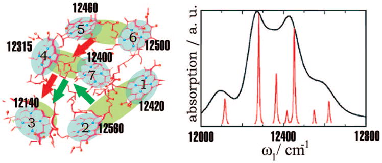
FMO complex structure of Chlorobium tepidum (left) and its simulated linear absorption (right), taken from ref 81 (eq 158).

Figure 11.

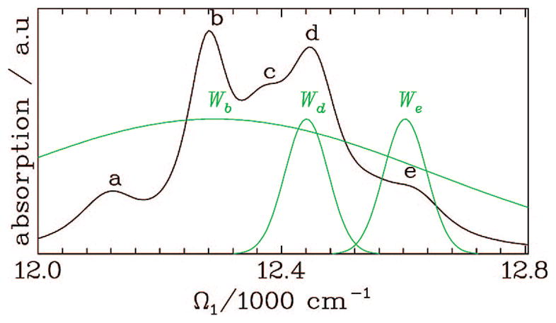
Linear absorption spectrum for FMO of Chlorobium tepidum. The 5 identifiable peaks a–e, where a is the lowest-energy absorption peak and e is the highest. The power spectra of the three excitation pulses (W_b, W_d, and W_e) used to calculate the signal in Figure 15. Pulse W_e excites band e only, pulse W_d excites band d only, and pulse W_b is broad and excites all bands.

10.1. Simulated Signals at the CED and MFA Levels

We start by neglecting transport and using the quasiparticle approach (eqs 127–129) with the scattering matrix eq 387 (MFA) or eq 92 (CED). We first assume broad pulse bandwidths, setting the pulse spectral envelopes to 1.

The MFA and CED S_kI signals at t₂ = 0 are compared in Figure 12. Since the two approaches are identical in the single-exciton space, the diagonal section, which shows the single excitons, is similar and reflects absorption peaks. However, their amplitudes are different.

Figure 12.

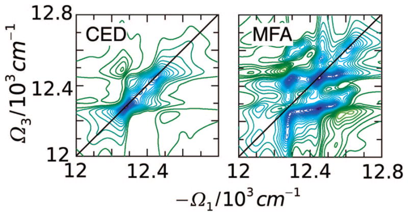
Im $S_{{\mathit{k}}_{\text{I}}}^{(\text{QP})}({\mathrm{\Omega }}_3,t_2,{\mathrm{\Omega }}_1)$ signal (imaginary part) in the MFA and CED for FMO at t₂ = 0 ps.

The large differences appear mostly in off-diagonal regions, where double-exciton properties show up. In the MFA, the two excitons evolve independently, and their correlations are neglected. Peak positions, which reflect the double-exciton energies, are then given by the combinations of single-exciton energies ε_e + ε_e′. The CED scattering matrix, in contrast, induces additional shifts of the resonant positions coming from exciton–exciton interactions.

A similar comparison is shown in Figures 13 and 14 for the double quantum coherence S_kIII signal.^83,205,206 It projects the double excitons directly on the Ω₂ axis, making it very sensitive to the fine features of the double-exciton manifold. The MFA provides an approximation to the double-exciton manifold by neglecting exciton–exciton correlation effects. The two peak patterns are mostly different in the higher-energy region (Ω₂ >24 800 cm⁻¹), where the MFA signal is featureless but the CED shows well-resolved peaks.

Figure 13.

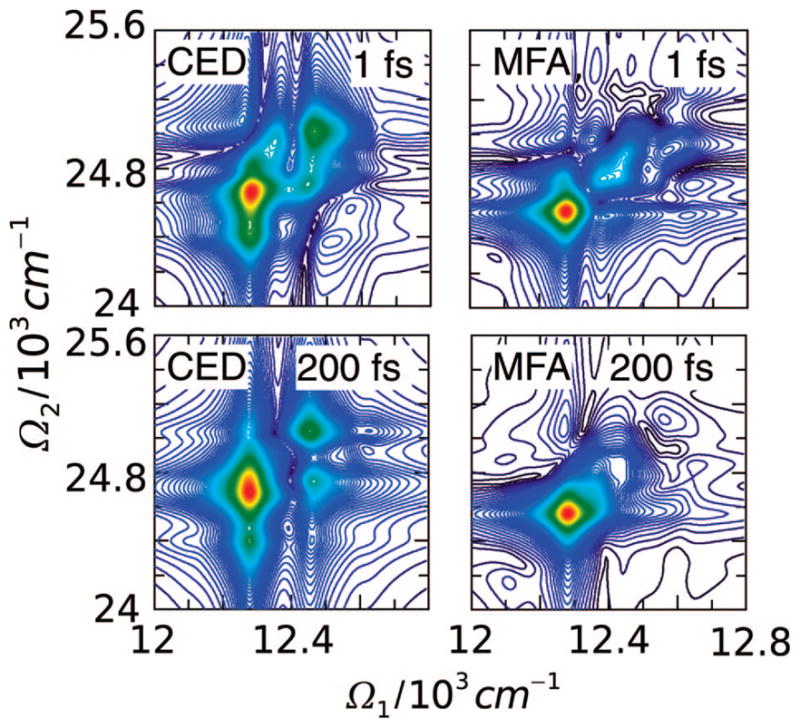
$\mid S_{{\mathit{k}}_{\text{III}}}^{(\text{QP})}(t_3,{\mathrm{\Omega }}_2,{\mathrm{\Omega }}_1)\mid$ signal in the MFA and CED for FMO at t₃ = 1 fs and t₃ = 200 fs.

Figure 14.

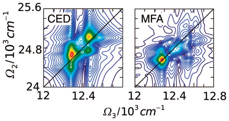
$\mid S_{{\mathit{k}}_{\text{III}}}^{(\text{QP})}({\mathrm{\Omega }}_3,{\mathrm{\Omega }}_2,t_1)\mid$ signal in the MFA and CED for FMO at t₁ = 0 fs.

The remainder of this section shows simulated k_I signals that go beyond the CED to include transport during t₂ at the secular Redfield theory level.

10.2. Dissecting Energy-Transfer Pathways by Using Finite-Pulse Bandwidths

The 2D signals were calculated using eq 127 and include transport during t₂. We used Gaussian pulse envelopes,

$${\mathbb{E}}_j(\omega )={\mathbb{E}}_j{\text{e}}^{-{(\omega /{\sigma }_j)}^2}.$$ (130)

In Figure 15, we show three finite-pulse simulations that demonstrate how a proper choice of the pulse envelopes, using information from the absorption spectrum, can be used to reveal the energy-transfer pathways, without any prior knowledge of the system’s Hamiltonian and parameters.

Figure 15.

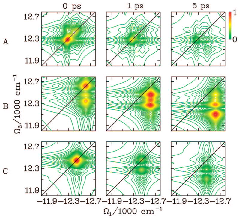
2D signal $\mid S_{{\mathit{k}}_{\text{I}}}^{(\text{QP})}({\mathrm{\Omega }}_3,t_2,{\mathrm{\Omega }}_1)\mid$ for the three experiments A, B, and C, as described in the text. (Top row, A) broad pulses; (Middle row, B) the first two pulses select the e band; (Bottom row, C) the first two pulses select the d band. The black line marks the diagonal. The pulses are shown in Figure 11.

Experiment A (top row) uses four broad pulses, whose power spectra are given by W_b in Figure 11 and cover the entire exciton band. At t₂ = 0 (left column of Figure 15), the k_I signal is dominated by two diagonal peaks corresponding to bands b and d. The cross-peaks are weak. As t₂ is increased, relaxation toward lower energies is observed; a higher-energy photon creates an excited state that decays toward lower-energy excited states, and the system emits at lower energies. At t₂ = 1 ps, cross-peaks start to appear below the diagonal. The cross-peak at (−Ω₁ = d, Ω₃ = b) shows that some excitation energy of the d band has been transported to b. The right panel (t₂ = 5 ps) shows additional cross-peaks. The (d, b) and (d, a) peaks indicate that energy from the d band has migrated to both the b and a bands. The absence of a diagonal (d, d) peak indicates that most of the initial exciton energy of the d band has decayed to lower-energy bands. The (b, a) peak is induced by energy transfer from b to a. Energy transport to the lowest excited state is completed in a few picoseconds. All energy-transfer pathways contribute to the signal; however, some are clearly dominant.

In Figure 15B, the first two pulses are narrow (W_e in Figure 11; σ_1/2 = 50 cm⁻¹ bandwidth) and selectively excite band e, and the last two pulses are broad (W_b). At t₂ = 0 ps, the pulses select peaks such that −Ω₁ lies in band e. The dominant diagonal peaks at (b, b) and (d, d) fall out of the pulse bandwidth, making weak cross-peaks more visible. At t₂ = 1 ps, the population created in band e has been transferred to b, c, and d (as seen from the larger (e, d), (e, c), and (e, b) cross-peak intensities) but not to the lower a band (no (e, a) cross-peak). After 5 ps, we see four cross-peaks indicating that all lower bands are populated, but the population of the higher energy states, especially d, is very small (weaker (e, d) and (e, c) cross-peaks). It is difficult to observe this pathway with broadband pulses (Figure 15A), since it is an order of magnitude weaker than the dominant one.

In Figure 15C, the first two pulses are narrow (W_d in Figure 11) and selectively excite the d band, but the last two pulses are broad. At t₂ = 0 ps, only the diagonal (d, d) peak is observed. As in Figure 15B, no significant excitation has been transferred to the lowest-energy band in 1 ps (no (d, a) cross-peak). What is different here is that only two bands are populated during the entire energy-transfer process (shown as the cross-peaks (d, b) and (d, a), the cross-peak at (d, c) never appears). The c band is not populated at t₂ = 5 ps even though its energy is lower than the original excitation, suggesting that the c and d bands correspond to localized excitations residing on different (and weakly coupled) sites. Similar conclusions were reached by Brixner et al.⁴⁰ who argued, by analyzing the exciton eigenvectors of a model system similar to ours, that the energy does not simply relax stepwise down the energy ladder.

10.3. Dissecting the Response Functions in Real Space

The third-order response function, whether calculated using the supermolecule or the quasiparticle approach, contains a product of four dipole moments associated with the various interactions with the fields. In order to analyze the NEE $R_{{\mathit{k}}_{\text{I}}}^{(\text{QP})}$ response function, eq 124, we shall transform the dipoles back to real space using μ_e = Σ_nψ_e,n μ_n with the single-exciton eigenstates ψ_e,n defined in section 9. We further single out the n₄ sum and write

$$R_{{\mathit{k}}_{\text{I}}}^{(\text{QP})}({\mathrm{\Omega }}_3,{\mathrm{\Omega }}_2,{\mathrm{\Omega }}_1)=\sum _{n_4}{R}_{{\mathit{k}}_{\text{I}},n_4}^{(\text{QP})}({\mathrm{\Omega }}_3,{\mathrm{\Omega }}_2,{\mathrm{\Omega }}_1),$$ (131)

with

$$R_{{\mathit{k}}_{\text{I}},n_4}^{(\text{QP})}({\mathrm{\Omega }}_3,{\mathrm{\Omega }}_2,{\mathrm{\Omega }}_1)=-2i{\mathit{\mu }}_{n_4}^{\ast }\sum _{e_4}{\psi }_{e_4{n}_4}\sum _{e_3{e}_2{e}_1}\sum _{e^{\prime }{e}^{″}}{\mathit{\mu }}_{e_3}{\mathit{\mu }}_{e_2}{\mathit{\mu }}_{e_1}^{\ast }\times G_{e_4}({\mathrm{\Omega }}_3){\mathrm{\Gamma }}_{e_4{e}^{\prime },e_3{e}^{″}}({\mathrm{\Omega }}_3+{\epsilon }_{e^{\prime }}+i{\gamma }_{e^{\prime }})\times {\mathbb{G}}_{e_3{e}^{″}}^{(0)}({\mathrm{\Omega }}_3+{\epsilon }_{e^{\prime }}+i{\gamma }_{e^{\prime }}){\mathbb{G}}_{e^{″}{e}^{\prime },e_2{e}_1}^{(N)}({\mathrm{\Omega }}_2)G_{e_1}^{\ast }(-{\mathrm{\Omega }}_1).$$ (132)

$R_{{\mathit{k}}_{\text{I}},n_4}^{(\text{QP})}$ gives the signal generated at site n₄. By varying t₂, we can further find the sites into which excitation energy flows, thus characterizing the population transport pathways and timescales in real space. Monitoring the energy transport in real-space is of particular interest in photosynthetic antennae, where the energy must eventually be funneled into specific sites (the reaction center).

A similar dissection procedure could be applied by singling out the third, second, or first interactions with the field (i.e., restricting the sums in eq 131 over n₃, n₂, and n₁, respectively) and calculating the contributions of each site to the various interactions. The linear absorption signal can be similarly dissected by singling out the second interaction (see eq 269):

$${\kappa }_{a,n_2}(\omega )\propto \omega \sum _e{\psi }_{n_2,e}{\mathit{\mu }}_{n_2}^{\ast }{\mathit{\mu }}_e\frac{{\gamma }_{eg}}{{(\omega -{\omega }_{eg})}^2+{\gamma }_{eg}^2}.$$ (133)

It gives the contribution of site n₂. The dissected absorption spectrum of FMO displayed in Figure 16 shows that the lowest-energy excited state (band a) is localized on chromophore 3, band b is on chromophores 4 and 7, and band d is delocalized over chromophores 5 and 6.

Figure 16.

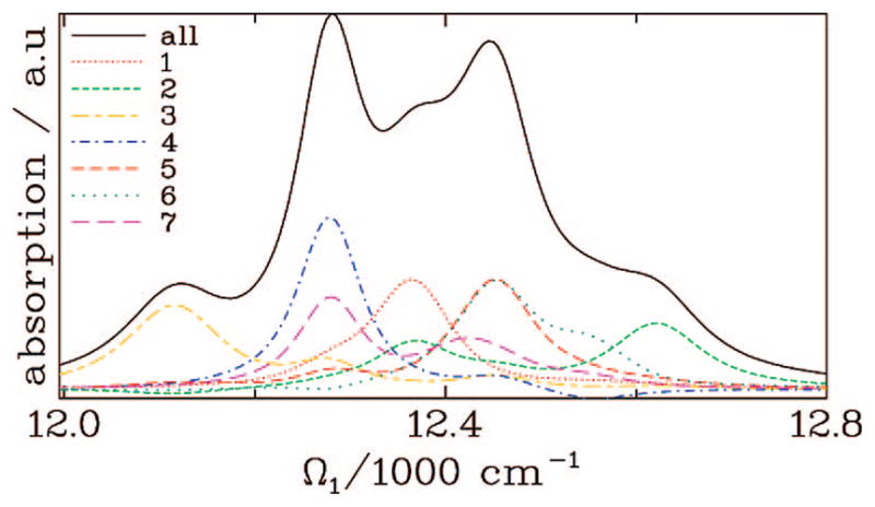
Absorption spectrum for FMO dissected into its seven chromophores by the last interaction with the field (eq 133). The contribution from each chromophore is given by a different color.

The $R_{{\mathit{k}}_{\text{I}},n_4}^{(\text{QP})}({\mathrm{\Omega }}_3,t_2=0,{\mathrm{\Omega }}_1)$ spectrum displayed in Figure 17 is dominated by chromophores 1, 4, 5, 6, and 7. As can also be seen from the absorption dissection, the (b, b) peak is delocalized over chromophores 4 and 7. The (d, d) peak is delocalized over sites 5 and 6, while (c, c) is localized on chromophore 1. For t₂ = 10 ps (Figure 18), the signal is generated at chromophores 3, 4, and 7. This is to be expected since excitation energy flows in a downhill path. Band a is localized on chromophore 3. Hence, the cross-peaks (d, a) and (b, a) are dominated by R_kI,3. The second lowest energy band, b, is still populated at t₂ = 10 ps. Hence, R_kI,4 and R_kI,7 still contribute to the response function since the b band is delocalized across sites 4 and 7. These contributions contain the two peaks at (b, b) (the b band is still populated) and (d, b) (exciton transfer from d to b).

Figure 17.

$R_{{\mathit{k}}_{\text{I}},n_4}^{(\text{QP})}({\mathrm{\Omega }}_3,t_2,{\mathrm{\Omega }}_1)$ signal (eq 132) for the FMO light-harvesting complex at t₂ = 0 ps. (Left column) The imaginary part of the response function; (Right column) the absolute value. The signal is dominated by chromophores 4, 5, 6, and 7 (Figure 10), which also dominate the two strongest bands (b and d) of the absorption spectrum. Chromophores 2 and 3 do not contribute significantly and were omitted. Color code is the same as in Figure 15.

Figure 18.

Same as Figure 17 but at t₂ = 10 ps. The signal is dominated by chromophores 3 and 4 (and a small contribution of 7), onto which the lowest excited states (3) and the second lowest excited states (4 and 7) are delocalized.

This dissection analysis provides similar information to the finite pulse envelope techniques discussed above. The difference is that here we select the chromophores, whereas the finite envelopes select the exciton eigenstates. The two are close when the eigenstates are localized. One can achieve a similar dissection using a broad band for the first three pulses and a narrow band for the last pulse.

This dissection analysis provides information that goes beyond the eigenvalues and the eigenvectors: it can be used to highlight specific energy-transfer pathways and timescales (as was done in section 10.2 using finite pulses) and find the dephasing rates of coherences between chromophores. Exciton delocalization can be characterized by the participation ratio,^182,207,208

$$L_e=\frac{1}{{\displaystyle \sum _n}{\mid {\psi }_{en}\mid }^4},$$ (134)

L_e varies between 1 and ℕ for an ℕ-chromophore aggregate and is a measure of the effective number of chromophores contributing to the exciton e. For FMO with the Hamiltonian parameters of ref 81, the participation ratios for the seven exciton states are (in increasing order of energy): L₁ = 1.3, L₂ = 2.3, L₃ = 1.6, L₄ = 1.8, L₅ = 2.4, L₆ = 2.8, and L₇ = 1.6. As expected, the lowest-energy exciton is localized on a single site (chromophore number 3). The other excitons are more delocalized, especially excitons 2, 5, and 6, which are delocalized on chromophores 4 and 7 (exciton 2), 5 and 6 (exciton 5), and 5 and 6 (exciton 6). Another useful measure is the coherence length,⁷⁰

$$L_{\rho }(t)=\frac{{({\displaystyle \sum _{nm}}\mid {\rho }_{mn}(t)\mid )}^2}{\mathbb{N}{\displaystyle \sum _{nm}}{\mid {\rho }_{mn}(t)\mid }^2},$$ (135)

which reveals the number of chromophores on which the exciton density matrix is delocalized along the antidiagonal direction.

The dissection analysis can be used to extract some additional measures of exciton-state delocalization. Let us consider the following quantity

$$L_d({\mathrm{\Omega }}_3,t_2,{\mathrm{\Omega }}_1)=\sum _{n_4}\mid R_{{\mathit{k}}_{\text{I}},n_4}^{(\text{QP})}({\mathrm{\Omega }}_3,t_2,{\mathrm{\Omega }}_1)\mid -\mid R_{{\mathit{k}}_{\text{I}}}^{(\text{QP})}({\mathrm{\Omega }}_3,t_2,{\mathrm{\Omega }}_1)\mid ,$$ (136)

where $R_{{\mathit{k}}_{\text{I}},n_4}^{(\text{QP})}({\mathrm{\Omega }}_3,t_2,{\mathrm{\Omega }}_1)$ is the contribution of the n₄th chromophore to the response function. L_d will vanish for regions dominated by a single chromophore and will grow with the degree of delocalization. In Figure 19, we display L_d at t₂ = 0 and t₂ = 10 ps. Obviously the diagonal peaks are localized on very few chromophores. This can be anticipated from our analysis of the linear absorption shown in Figure 16. The cross-peaks in Figure 19 for t₂ = 10 ps are more delocalized because they result from population transfer facilitated by exciton delocalization (c.f., eq 370).

Figure 19.

(Left column) Absolute value of the response function, $\mid R_{{\mathit{k}}_{\text{I}}}^{(\text{QP})}({\mathrm{\Omega }}_3,t_2,{\mathrm{\Omega }}_1)\mid$ (eq 124). (Middle column) The sum of the absolute value of the dissected response function, ${\sum }_{n_4}\mid R_{{\mathit{k}}_{\text{I}},n_4}^{(\text{QP})}({\mathrm{\Omega }}_3,t_2,{\mathrm{\Omega }}_1)\mid$ (eq 132). (Right column) The delocalization length, L_d(Ω₃, t₂, Ω₁) (eq 136). The delay time t₂ = 0 (top) and 10 ps (bottom). Color code is the same as in Figure 15.

10.4. Signatures of Quartic Exciton Couplings

The quadratic excitonic couplings J_mn in eq 58 correspond to the “strong J coupling” regime in homonuclear NMR. Chromophores coupled through negative (positive) couplings form J (H) aggregates. The quartic couplings are analogous to the Darling–Dennison coupling²⁰⁹ in infrared spectroscopy and are known as the “weak (heteronuclear) coupling” of heteronuclear NMR. A detailed comparison between NMR and multidimensional infrared and optical spectroscopy was given in refs ⁵⁷ and ⁵⁸. The FMO simulations presented so far assumed that each chlorophyll is a two-level chromophore, setting = 0 and Δ_m → ∞. This anharmonic penalty prevents two excitations from residing on the same site.

Here we study the possible signatures of .²¹⁰ The energy of two-exciton states for excitations on sites m and n (i.e., E_m,n = 〈Φ_fmn|Ĥ_S|Φ _fmn〉, with Φ _fmn defined in section 6) is

$$E_{m,n}{\hslash }^{-1}={\epsilon }_m+{\epsilon }_n+{\mathbb{K}}_{mn}(1-{\delta }_{mn})+{\mathrm{\Delta }}_m{\delta }_{mn}.$$ (137)

The coupling implies that double excitations on neighboring sites have lower (negative ; exciton attraction) or higher (positive ; exciton repulsion) energy compared to the sum of energies of the two single excitations. In the NEE, enters solely through the scattering matrix. For finite , the coherent time-evolution of the Y variables will show resonances shifted by couplings.

To demonstrate the possible effects of these off-diagonal quartic couplings, we have switched on the quartic coupling between the fourth and fifth chromophores in FMO. These sites are chosen because they contribute significantly to the strong b and d absorption bands (Figure 11), as can be easily seen from the dissected linear absorption spectrum (Figure 16). This is a simple illustration of possible signature of the coupling, which we use as a free parameter. Figure 20 depicts the k_I signals calculated with the NEE for = = ±300 cm⁻¹ and t₂ = 0.

Figure 20.

Effects of the off-diagonal quartic coupling, , on the k_I spectra for t₂ = 0. (Left column) The imaginary part of the response function; (Right column) absolute value. From top to bottom, = = 0, +300, −300 cm⁻¹. Color code is the same as in Figure 15.

Effects of the quartic couplings are most easily explained by looking at the SOS expressions for the response function of a dimer,

$$R_{{\mathit{k}}_{\text{I}}}^{(\text{SOS})}({\mathrm{\Omega }}_3,t_2=0,{\mathrm{\Omega }}_1)=R_{{\mathit{k}}_{\text{I}}}^{(\text{GSB})}({\mathrm{\Omega }}_3,t_2=0,{\mathrm{\Omega }}_1)+R_{{\mathit{k}}_{\text{I}}}^{(\text{ESE})}({\mathrm{\Omega }}_3,t_2=0,{\mathrm{\Omega }}_1)+R_{{\mathit{k}}_{\text{I}}}^{(\text{ESA})}({\mathrm{\Omega }}_3,t_2=0,{\mathrm{\Omega }}_1),$$ (138)

where

$$R_{{\mathit{k}}_{\text{I}}}^{(\text{GSB})}({\mathrm{\Omega }}_3,t_2=0,{\mathrm{\Omega }}_1)=R_{{\mathit{k}}_{\text{I}}}^{(\text{ESE})}({\mathrm{\Omega }}_3,t_2=0,{\mathrm{\Omega }}_1)=-{\left(\frac{i}{\hslash }\right)}^3\left[\frac{{\mid {\mathit{\mu }}_{+}\mid }^4}{({\mathrm{\Omega }}_3-{\epsilon }_{+}+i{\gamma }_{+})({\mathrm{\Omega }}_1+{\epsilon }_{+}+i{\gamma }_{+})}+\frac{{\mid {\mathit{\mu }}_{-}\mid }^4}{({\mathrm{\Omega }}_3-{\epsilon }_{-}+i{\gamma }_{-})({\mathrm{\Omega }}_1+{\epsilon }_{-}+i{\gamma }_{-})}+\frac{{\mid {\mathit{\mu }}_{-}\mid }^2{\mid {\mathit{\mu }}_{+}\mid }^2}{({\mathrm{\Omega }}_3-{\epsilon }_{+}+i{\gamma }_{+})({\mathrm{\Omega }}_1+{\epsilon }_{-}+i{\gamma }_{-})}+\frac{{\mid {\mathit{\mu }}_{-}\mid }^2{\mid {\mathit{\mu }}_{+}\mid }^2}{({\mathrm{\Omega }}_3-{\epsilon }_{-}+i{\gamma }_{-})({\mathrm{\Omega }}_1+{\epsilon }_{+}+i{\gamma }_{+})}\right],$$ (139)

$$R_{{\mathit{k}}_{\text{I}}}^{(\text{ESA})}({\mathrm{\Omega }}_3,t_2=0,{\mathrm{\Omega }}_1)={\left(\frac{i}{\hslash }\right)}^3\left[\frac{({\mathit{\mu }}_{+}^2{\mathit{\mu }}_{f,+}^2+{\mathit{\mu }}_{-}{\mathit{\mu }}_{f,-}{\mathit{\mu }}_{+}{\mathit{\mu }}_{f,+})}{({\mathrm{\Omega }}_3-{\epsilon }_{-}+\mathbb{K}+i{\gamma }_{f,+})({\mathrm{\Omega }}_1+{\epsilon }_{+}+i{\gamma }_{+})}+\frac{({\mathit{\mu }}_{-}^2{\mathit{\mu }}_{f,-}^2+{\mathit{\mu }}_{-}{\mathit{\mu }}_{f,-}{\mathit{\mu }}_{+}{\mathit{\mu }}_{f,+})}{({\mathrm{\Omega }}_3-{\epsilon }_{+}+\mathbb{K}+i{\gamma }_{f,-})({\mathrm{\Omega }}_1+{\epsilon }_{-}+i{\gamma }_{-})}\right],$$ (140)

where μ_± are the transition dipoles between the ground and one of the single-excited states (“+” and “−”). They are related to the dipoles in the local basis by the following transformation: μ_± = Ψ_±,1μ₁ + Ψ_±,2μ₂. The dimer model has a single doubly excited state, f, with energy ε₊ + ε₋ + , and the transition dipole between the singly-excited and the double-excited state is μ_f,± = Ψ_±,1μ₂ +Ψ_±,2μ₁. The two terms of eq 140 are ESA contributions. The quartic coupling enters only in these terms.

As can be seen from eq 139, the GSB and ESE contributions to the cross-peaks interfere with the ESA. Hence, the cross-peaks at (ε₊, ε₋) and (ε₋, ε₊) interfere destructively. As is increased, the ESA peaks are shifted along Ω₃ by and the cross-peaks no longer cancel out, creating a doublet.

A similar splitting of the cross-peaks is expected in larger aggregates. This explains the trends seen in Figure 20. When = 0, the diagonal peaks (b, b) and (d, d) dominate. As is turned on, the GSB and ESE contributions to the cross-peaks shift spectrally and no longer interfere with the ESA and the cross-peaks at (b, d) and (d, b) appear. Furthermore, the ESA cross-peak can be observed as weaker peaks shifted along Ω₃ (these regions are circled in Figure 20). These cross-peaks appear at (b, d + ) and (d, b + ).

Signatures of the off-diagonal quartic couplings are also manifest for t₂ > 0. In Figure 21, we show the k_I response function for different as in Figure 20 but for t₂ = 10 ps. The b band is still populated even after long t₂. This is evident from the large diagonal peak in the b region for = 0, shown in the top panel of Figure 21. Hence, the fourth site is populated since band b corresponds to an exciton localized mainly on this site. For = −300 cm⁻¹, the doubly excited Φ_f45 state is energetically favored. The excitation energy, absorbed in the b or d band, which relaxes to b during t₂, can re-emit from the d band, leading to a high-energy diagonal peak and corresponding cross-peaks. Since the doubly excited state Φ_f45 is blue-shifted when = +300 cm⁻¹, these new features are weaker in the second row of Figure 21. In this case, the anharmonic coupling shifts the ESA contributions for the high-energy diagonal peak (d, d) and for the (b, d) cross-peak along Ω₃.

Figure 21.

Same as in Figure 20, but at t₂ = 10 ps.

11. Interplay of Transport and Slow Fluctuations in the Third-Order Response

In section 7, we have derived quasiparticle expressions for the exciton-response functions by assuming fast fluctuations of the bath, which justifies the Markovian approximation for relaxation. This leads to a Pauli rate equation for populations and dephasing of exciton coherences. The supermolecule approach, in contrast, can describe the coupling to a bath with a broad range of fluctuation timescales. This higher-level treatment requires the explicit calculation of two-exciton eigenstates, which is only feasible in small aggregates. Fortunately, the detailed bath dynamics can be typically observed only in small systems where the electronic spectra are not too congested.

It was shown in section 3 that the resonant Liouville space pathways can be classified into ESE, ESA, and GSB types. The secular approximation for the Green’s function additionally decouples coherences and populations. The response function may then be partitioned into contributions of coherences C and populations P during t₂.

The resonant contributions to each technique are given by the Feynman diagrams of Figures 4–7. In the following expressions, we will use the same labeling for the various terms used in the diagrams: ia, ii, iiia, iva, v, and via are purely population contributions, and ib, iiib, ivb, vib, vii, and viii are purely coherence contributions.

The k_I response function will be recast in the form:

$$R_{{\mathit{k}}_{\text{I}},\text{ia}}(t_3,t_2,t_1)=-i{\hslash }^{-3}\theta (t_1)\theta (t_2)\theta (t_3)\sum _{e,e^{\prime }}{\mathit{\mu }}_{g{e}^{\prime }}{\mathit{\mu }}_{e^{\prime }g}{\mathit{\mu }}_{eg}{\mathit{\mu }}_{ge}\times {\mathbb{G}}_{e^{\prime }{e}^{\prime },ee}^{(N)}(t_2)exp[-i{\xi }_{e^{\prime }g}{t}_3-i{\xi }_{ge}{t}_1+{\varphi }_{e^{\prime }e}^{(\text{ia})}(t_3,t_2,t_1)],$$ (141)

$$R_{{\mathit{k}}_{\text{I}},\text{ib}}(t_3,t_2,t_1)=-i{\hslash }^{-3}\theta (t_1)\theta (t_2)\theta (t_3)\sum _{e,e^{\prime }}^{e\ne e^{\prime }}{\mathit{\mu }}_{g{e}^{\prime }}{\mathit{\mu }}_{eg}{\mathit{\mu }}_{e^{\prime }g}{\mathit{\mu }}_{ge}\times exp[-i{\xi }_{e^{\prime }g}{t}_3-i{\xi }_{e^{\prime }e}{t}_2-i{\xi }_{ge}{t}_1+{\varphi }_{e^{\prime }e}^{(\text{ib})}(t_3,t_2,t_1)],$$ (142)

$$R_{{\mathit{k}}_{\text{I}},\text{ii}}(t_3,t_2,t_1)=-i{\hslash }^{-3}\theta (t_1)\theta (t_2)\theta (t_3)\sum _{e^{\prime },e}{\mathit{\mu }}_{g{e}^{\prime }}{\mathit{\mu }}_{e^{\prime }g}{\mathit{\mu }}_{eg}{\mathit{\mu }}_{ge}\times exp[-i{\xi }_{e^{\prime }g}{t}_3-i{\xi }_{ge}{t}_1+{\varphi }_{e^{\prime }e}^{(\text{ii})}(t_3,t_2,t_1)],$$ (143)

$$R_{{\mathit{k}}_{\text{I}},\text{iiia}}(t_3,t_2,t_1)=+i{\hslash }^{-3}\theta (t_1)\theta (t_2)\theta (t_3)\sum _{e,e^{\prime },f}{\mathit{\mu }}_{e^{\prime }f}{\mathit{\mu }}_{f{e}^{\prime }}{\mathit{\mu }}_{eg}{\mathit{\mu }}_{ge}\times {\mathbb{G}}_{e^{\prime }{e}^{\prime },ee}^{(N)}(t_2)exp[-i{\xi }_{f{e}^{\prime }}{t}_3-i{\xi }_{ge}{t}_1+{\varphi }_{f{e}^{\prime }e}^{(\text{iiia})}(t_3,t_2,t_1)],$$ (144)

$$R_{{\mathit{k}}_{\text{I}},\text{iiib}}(t_3,t_2,t_1)=+i{\hslash }^{-3}\theta (t_1)\theta (t_2)\theta (t_3)\sum _{e,e^{\prime },f}^{e\ne e^{\prime }}{\mathit{\mu }}_{ef}{\mathit{\mu }}_{f{e}^{\prime }}{\mathit{\mu }}_{e^{\prime }g}{\mathit{\mu }}_{ge}\times exp[-i{\xi }_{fe}{t}_3-i{\xi }_{e^{\prime }e}{t}_2-i{\xi }_{ge}{t}_1+{\varphi }_{f{e}^{\prime }e}^{(\text{iiib})}(t_3,t_2,t_1)].$$ (145)

As in section 4, we define the complex transition frequencies

$${\xi }_{ab}\equiv {\epsilon }_a-{\epsilon }_b-i({\tau }_a^{-1}+{\tau }_b^{-1})/2,$$ (146)

where τ_a is the lifetime of state a. ϕ(t₃, t₂, t₁) are multipoint line-shape functions induced by bath fluctuations. These are responsible for all other dephasing mechanisms beyond the lifetimes τ.

Similarly, we recast the k_II response in the form:

$$R_{{\mathit{k}}_{\text{II}},\text{iva}}(t_3,t_2,t_1)=-i{\hslash }^{-3}\theta (t_1)\theta (t_2)\theta (t_3)\sum _{e,e^{\prime }}{\mathit{\mu }}_{g{e}^{\prime }}{\mathit{\mu }}_{e^{\prime }g}{\mathit{\mu }}_{ge}{\mathit{\mu }}_{eg}\times {\mathbb{G}}_{e^{\prime }{e}^{\prime },ee}^{(N)}(t_2)exp[-i{\xi }_{e^{\prime }g}{t}_3-i{\xi }_{eg}{t}_1+{\varphi }_{e^{\prime }e}^{(\text{iva})}(t_3,t_2,t_1)],$$ (147)

$$R_{{\mathit{k}}_{\text{II}},\text{ivb}}(t_3,t_2,t_1)=-i{\hslash }^{-3}\theta (t_1)\theta (t_2)\theta (t_3)\sum _{e,e^{\prime }}^{e\ne e^{\prime }}{\mathit{\mu }}_{ge}{\mathit{\mu }}_{e^{\prime }g}{\mathit{\mu }}_{g{e}^{\prime }}{\mathit{\mu }}_{eg}\times exp[-i{\xi }_{eg}{t}_3-i{\xi }_{{ee}^{\prime }}{t}_2-i{\xi }_{eg}{t}_1+{\varphi }_{e^{\prime }e}^{(\text{ivb})}(t_3,t_2,t_1)],$$ (148)

$$R_{{\mathit{k}}_{\text{II}},\text{v}}(t_3,t_2,t_1)=-i{\hslash }^{-3}\theta (t_1)\theta (t_2)\theta (t_3)\sum _{e^{\prime },e}{\mathit{\mu }}_{g{e}^{\prime }}{\mathit{\mu }}_{e^{\prime }g}{\mathit{\mu }}_{ge}{\mathit{\mu }}_{eg}\times exp[-i{\xi }_{e^{\prime }g}{t}_3-i{\xi }_{eg}{t}_1+{\varphi }_{e^{\prime }e}^{(\text{v})}(t_3,t_2,t_1)],$$ (149)

$$R_{{\mathit{k}}_{\text{II}},\text{via}}(t_3,t_2,t_1)=+i{\hslash }^{-3}\theta (t_1)\theta (t_2)\theta (t_3)\sum _{e,e^{\prime }f}{\mathit{\mu }}_{e^{\prime }f}{\mathit{\mu }}_{f{e}^{\prime }}{\mathit{\mu }}_{ge}{\mathit{\mu }}_{eg}\times {\mathbb{G}}_{e^{\prime }{e}^{\prime },ee}^{(N)}(t_2)exp[-i{\xi }_{f{e}^{\prime }}{t}_3-i{\xi }_{eg}{t}_1+{\varphi }_{f{e}^{\prime }e}^{(\text{via})}(t_3,t_2,t_1)],$$ (150)

$$R_{{\mathit{k}}_{\text{II}},\text{vib}}(t_3,t_2,t_1)=+i{\hslash }^{-3}\theta (t_1)\theta (t_2)\theta (t_3)\sum _{e,e^{\prime },f}^{e\ne e^{\prime }}{\mathit{\mu }}_{e^{\prime }f}{\mathit{\mu }}_{fe}{\mathit{\mu }}_{g{e}^{\prime }}{\mathit{\mu }}_{eg}\times exp[-i{\xi }_{f{e}^{\prime }}{t}_3-i{\xi }_{{ee}^{\prime }}{t}_2-i{\xi }_{eg}{t}_1+{\varphi }_{f{e}^{\prime }e}^{(\text{vib})}(t_3,t_2,t_1)].$$ (151)

Finally, k_III is composed of ESA₁ and ESA₂ (both are coherent contributions since populations are not created in k_III):

$$R_{{\mathit{k}}_{\text{III}},\text{vii}}(t_3,t_2,t_1)=+i{\hslash }^{-3}\theta (t_1)\theta (t_2)\theta (t_3)\sum _{e,e^{\prime },f}{\mathit{\mu }}_{e^{\prime }f}{\mathit{\mu }}_{g{e}^{\prime }}{\mathit{\mu }}_{fe}{\mathit{\mu }}_{eg}\times exp[-i{\xi }_{f{e}^{\prime }}{t}_3-i{\xi }_{fg}{t}_2-i{\xi }_{eg}{t}_1+{\varphi }_{f{e}^{\prime }e}^{(\text{vii})}(t_3,t_2,t_1)],$$ (152)

$$R_{{\mathit{k}}_{\text{III}},\text{viii}}(t_3,t_2,t_1)=-i{\hslash }^{-3}\theta (t_1)\theta (t_2)\theta (t_3)\sum _{e,e^{\prime },f}{\mathit{\mu }}_{g{e}^{\prime }}{\mathit{\mu }}_{e^{\prime }f}{\mathit{\mu }}_{fe}{\mathit{\mu }}_{eg}\times exp[-i{\xi }_{e^{\prime }g}{t}_3-i{\xi }_{fg}{t}_2-i{\xi }_{eg}{t}_1+{\varphi }_{f{e}^{\prime }e}^{(\text{viii})}(t_3,t_2,t_1)].$$ (153)

In the coming sections, we shall derive microscopically and extend all quantities appearing in the phenomenological expressions of section 4. The results of three approximations will be recast in the form of eqs 141–153 and will only differ by the phase functions ϕ that will be given by eqs 166, 177, and 179. The response function expressions of section 4 are recovered by setting all ϕ = 0 and assuming that the dephasing is caused by finite lifetimes + pure dephasing in the Markovian approximation.

11.1. Coherent Exciton Dynamics; Diagonal Gaussian Fluctuations with Arbitrary Timescale

We assume that the system is described by the Hamiltonian equation (eq 94) with the system part in the form of eq 2 and the harmonic bath model given by eq 95. We partition Ĥ = Σ_υ|υ〉Ĥ_υ〈υ|, where the bath operator Ĥ_υ characterizes the bath-induced perturbation of the energy of system state υ,

$${\widehat{H}}_v={\hslash }^{-1}\langle v\mid \widehat{H}\mid v\rangle ={\epsilon }_v+{\widehat{q}}_{vv}+{\widehat{H}}_B,$$ (154)

q̂_υυ is a collective bath coordinate:

$${\widehat{q}}_{vv}\equiv {\hslash }^{-1}\langle v\mid {\widehat{H}}_{SB}\mid v\rangle =\sum _{\alpha }{d}_{vv,\alpha }({\widehat{a}}_{\alpha }^{†}+{\widehat{a}}_{\alpha }).$$ (155)

q̂_υυ induces the frequency fluctuations of state υ with respect to the reference Hamiltonian of state a:

$${\widehat{q}}_{vv}^{(a)}(t)\equiv {\text{e}}^{i{\hslash }^{-1}{\widehat{H}}_{a}t}{\widehat{q}}_{vv}{\text{e}}^{-i{\hslash }^{-1}{\widehat{H}}_{a}t}.$$ (156)

Off-diagonal fluctuations responsible for population relaxation are neglected. The arguments presented here hold in the eigenstate-basis, where all off-diagonal elements of the Hamiltonian vanish. However, for coupled molecular aggregates, both diagonal and off-diagonal fluctuations in real-space representation lead to transport, since they result in nonzero off-diagonal Hamiltonian fluctuations in an arbitrary reference basis set. This model was studied in refs ¹⁰⁰ and ¹¹². Here, we present the final expressions for the exciton model of Figure 3. In this subsection, unlike the rest of the review, we do not make the RWA for the response function. This allows for more compact expressions. The RWA is only invoked for the final results (eq 166).

The linear and third-order response functions can be calculated exactly from eqs 12 and 15 using the second-order cumulant expansion.^52,112 This is known as the CGF: cumulant expansion of Gaussian fluctuations.

The linear response function is given by

$$R^{(1)}(t)=\frac{i}{\hslash }[\mathbb{J}(t)-{\mathbb{J}}^{\ast }(t)],$$ (157)

where (τ₂ − τ₁) = 〈μ̂ (τ₂)μ̂ (τ₁)〉 is the two-point dipole correlation function. The angular brackets imply equilibrium statistical averaging over the bath. is calculated exactly for this model:

$$\mathbb{J}(t)=\sum _{ab}{\mathit{\mu }}_{ab}{\mathit{\mu }}_{ba}{\rho }_{a}exp[-i{\omega }_{ba}t-g_{bb}(t)-g_{aa}(t)+g_{ab}(t)+g_{ba}(t)].$$ (158)

Here, ρ_a is the equilibrium population of state a, and we have introduced the line-shape function

$$g_{v{v}^{\prime }}(t)={\int }_0^t\text{d}{\tau }_2{\int }_0^{{\tau }_2}\text{d}{\tau }_1{C}_{v{v}^{\prime }}({\tau }_2-{\tau }_1).$$ (159)

$C_{v{v}^{\prime }}({\tau }_2-{\tau }_1)\equiv \langle {\widehat{q}}_{vv}^{(g)}({\tau }_2){\widehat{q}}_{v^{\prime }{v}^{\prime }}^{(g)}({\tau }_1)\rangle$ is the correlation function of bath fluctuations whose time evolution is given by the ground-state Hamiltonian. The line-shape function can be alternatively recast in terms of the spectral density,

$$C_{v{v}^{\prime }}^{″}(\omega )=\frac{1}{2}{\int }_0^{\infty }\text{d}texp(i\omega t)\langle [{\widehat{q}}_{vv}^{(g)}(t),{\widehat{q}}_{v^{\prime }{v}^{\prime }}^{(g)}(0)]\rangle ;$$ (160)

see eq 342 and 353. Its symmetries and other properties are summarized in Appendix F. We then have

$$g_{v{v}^{\prime }}(t)=\int \frac{\text{d}\omega }{2\pi }\frac{C_{v{v}^{\prime }}^{″}(\omega )}{{\omega }^2}[coth\left(\frac{\beta \hslash \omega }{2}\right)(1-cos\omega t)+isin\omega t-i\omega t].$$ (161)

The cumulant expansion similarly gives for the third-order response function,

$$R^{(3)}(t_3,t_2,t_1)={\left(\frac{i}{\hslash }\right)}^3[F(t_1,t_1+t_2,t_1+t_2+t_3,0)+F(0,t_1+t_2,t_1+t_2+t_3,t_1)+F(0,t_1,t_1+t_2+t_3,t_1+t_2)+F(t_1+t_2+t_3,t_1+t_2,t_1,0)]+c.c.,$$ (162)

where

$$F({\tau }_4,{\tau }_3,{\tau }_2,{\tau }_1)=\langle \widehat{\mathit{\mu }}({\tau }_4)\widehat{\mathit{\mu }}({\tau }_3)\widehat{\mathit{\mu }}({\tau }_2)\widehat{\mathit{\mu }}({\tau }_1)\rangle$$ (163)

is the four-point correlation function of the dipole operator in the Heisenberg picture (because we did not select pathways by invoking the RWA, R⁽³⁾ is now independent of the wavevector k_s). Expansion in the exciton eigenstates yields

$$F({\tau }_4,{\tau }_3,{\tau }_2,{\tau }_1)=\sum _{\mathit{dcba}}{\rho }_a{\mathit{\mu }}_{ad}{\mathit{\mu }}_{dc}{\mathit{\mu }}_{cb}{\mathit{\mu }}_{ba}exp[-i({\omega }_{da}{\tau }_{43}+{\omega }_{ca}{\tau }_{32}+{\omega }_{ba}{\tau }_{21})+{\phi }_{\mathit{dcba}}({\tau }_4,{\tau }_3,{\tau }_2,{\tau }_1)],$$ (164)

where φ_dcba(τ₄,τ₃,τ₂,τ₁) is a four-point line-shape function. For our harmonic bath model, we get

$${\phi }_{\mathit{cbag}}({\tau }_4,{\tau }_3,{\tau }_2,{\tau }_1)=-g_{cc}({\tau }_{43})-g_{bb}({\tau }_{32})-g_{aa}({\tau }_{21})-g_{cb}({\tau }_{42})+g_{cb}({\tau }_{43})+g_{cb}({\tau }_{32})-g_{ca}({\tau }_{41})+g_{ca}({\tau }_{42})+g_{ca}({\tau }_{31})-g_{ca}({\tau }_{32})-g_{ba}({\tau }_{31})+g_{ba}({\tau }_{32})+g_{ba}({\tau }_{21}),$$ (165)

where τ_ij = τ_i − τ_j. The expressions given in ref 100 were derived in the semiclassical limit, 〈ω_ab(t)ω_ab(0)〉 = 〈ω_ab(0)ω_ab(t) 〉; here, we do not invoke that approximation.²⁴ It is important to note that φ does depend on the ground-state index g, even though it does not appear explicitly in the right-hand side (rhs), since all time evolutions are calculated with the ground-state reference Hamiltonian (eq 160).

By invoking the RWA, we can now select the resonant contributions in the response function, as warranted for each technique. The resulting response functions then assume the form of eqs 141–153 with ${\mathbb{G}}_{e^{\prime }{e}^{\prime },ee}^{(N)}(t)=\theta (t){\delta }_{e^{\prime }e}$ and no lifetime broadening τ⁻¹ = 0. The phase functions are given by

$$\begin{array}{l}{\varphi }_{ee}^{(\text{ia})}(t_3,t_2,t_1)={\phi }_{\mathit{egeg}}^{\ast }(t_1,t_1+t_2+t_3,t_1+t_2,0),\\ {\varphi }_{e^{\prime }e}^{(\text{ii})}(t_3,t_2,t_1)={\phi }_{e^{\prime }\mathit{geg}}^{\ast }(t_1+t_2,t_1+t_2+t_3,t_1,0),\\ {\varphi }_{\mathit{fee}}^{(\text{iiia})}(t_3,t_2,t_1)={\phi }_{\mathit{efeg}}^{\ast }(t_1,t_1+t_2,t_1+t_2+t_3,0),\\ {\varphi }_{e^{\prime }e}^{(\text{ib})}(t_3,t_2,t_1)={\phi }_{e^{\prime }\mathit{geg}}^{\ast }(t_1,t_1+t_2+t_3,t_1+t_2,0),\\ {\varphi }_{f{e}^{\prime }e}^{(\text{iiib})}(t_3,t_2,t_1)={\phi }_{e^{\prime }\mathit{feg}}^{\ast }(t_1,t_1+t_2,t_1+t_2+t_3,0),\\ {\varphi }_{ee}^{(\text{iva})}(t_3,t_2,t_1)={\phi }_{\mathit{egeg}}(t_1,t_1+t_2,t_1+t_2+t_3,0),\\ {\varphi }_{e^{\prime }e}^{(\text{v})}(t_3,t_2,t_1)={\phi }_{e^{\prime }\mathit{geg}}(t_1+t_2+t_3,t_1+t_2,t_1,0),\\ {\varphi }_{\mathit{fee}}^{(\text{via})}(t_3,t_2,t_1)={\phi }_{\mathit{efeg}}(t_1,t_1+t_2+t_3,t_1+t_2,0),\\ {\varphi }_{e^{\prime }e}^{(\text{ivb})}(t_3,t_2,t_1)={\phi }_{e^{\prime }\mathit{geg}}(t_1,t_1+t_2,t_1+t_2+t_3,0),\\ {\varphi }_{f{e}^{\prime }e}^{(\text{vib})}(t_3,t_2,t_1)={\phi }_{e^{\prime }\mathit{feg}}(t_1,t_1+t_2+t_3,t_1+t_2,0),\\ {\varphi }_{f{e}^{\prime }e}^{(\text{vii})}(t_3,t_2,t_1)={\phi }_{e^{\prime }\mathit{feg}}(t_1+t_2,t_1+t_2+t_3,t_1,0),\\ {\varphi }_{f{e}^{\prime }e}^{(\text{viii})}(t_3,t_2,t_1)={\phi }_{e^{\prime }\mathit{feg}}(t_1+t_2+t_3,t_1+t_2,t_1,0).\end{array}$$ (166)

The line-shape function can be calculated analytically for certain models of the bath spectral density. Commonly used examples are Ohmic, white-noise, and Brownian oscillator spectral densities. The overdamped Brownian oscillator spectral density, defined by

$$C_{v{v}^{\prime }}^{″}(\omega )=2{\lambda }_{v{v}^{\prime }}\frac{\omega \mathrm{\Lambda }}{{\omega }^2+{\mathrm{\Lambda }}^2},$$ (167)

where Λ ⁻¹ is the fluctuation time scale and λ is the system–bath coupling strength, provides a simple expression for the line-shape function for t > 0 (for more details, see Appendix G),

$$g_{v{v}^{\prime }}(t)=\frac{{\lambda }_{v{v}^{\prime }}}{\mathrm{\Lambda }}coth(\hslash \mathrm{\Lambda }\beta /2)[exp(-\mathrm{\Lambda }t)+\mathrm{\Lambda }t-1]+\frac{4{\lambda }_{vv\text{'}}\mathrm{\Lambda }}{\hslash \beta }\sum _{n=1}^{\infty }\frac{{\text{e}}^{-{\nu }_{n}t}+{\nu }_{n}t-1}{{\nu }_n({\nu }_n^2-{\mathrm{\Lambda }}^2)}-i\frac{{\lambda }_{v{v}^{\prime }}}{\mathrm{\Lambda }}[exp(-\mathrm{\Lambda }t)+\mathrm{\Lambda }t-1],$$ (168)

where β = (k_BT)⁻¹ and ν_n = (2πn)/(ℏβ) are known as the Matsubara frequencies. For negative times, we have $g_{v{v}^{\prime }}(-t)=g_{v^{\prime }v}^{\ast }(t)$. The second term is a low-temperature correction, given by the additional Matsubara oscillators. The third term is responsible for bath-induced transition frequency shift. In the high-temperature limit, k_BT ≫ ℏΛ, we have

$$g_{v{v}^{\prime }}(t)=\frac{{\lambda }_{v{v}^{\prime }}}{\mathrm{\Lambda }}\left(\frac{2k_{\text{B}}T}{\hslash \mathrm{\Lambda }}-i\right)(exp(-\mathrm{\Lambda }t)+\mathrm{\Lambda }t-1).$$ (169)

11.2. Response with Population-Transport and Intermediate-Timescale Bath Fluctuations

The results of the previous section hold for purely diagonal (frequency) fluctuations with arbitrary timescales; population relaxation caused by off-diagonal fluctuations has been neglected. The Redfield equations, on the other hand, include transport but are limited to fast fluctuations. Here, we present approximate expressions, which include exciton transport and intermediate timescale fluctuations.

Dephasing occurs during the delay times t₁ and t₃, whereas transport takes place during t₂. Typically t₁,t₃ ≪t₂ (for photosynthetic complexes, population transport occurs in 500 fs-10 ps, while the coherence time scale is 100–300 fs). We assume an intermediate bath fluctuation time: fast compared to the transport but slow or comparable to the coherence-dephasing time. In this case, we can use the doorway-window representation of the response function and project the doorway and window functions onto the population/coherence blocks of the density matrix.^{184,185,211,212}

Populations are created during t₂ only in the k_I and k_II techniques. We therefore focus on these techniques. We first recast the response function, eq 15, in the form

$$R^{(3)}(t_3,t_2,t_1)={\left(\frac{i}{\hslash }\right)}^{3}Tr[\mathbb{W}(t_3)\mathbb{G}(t_2)\mathbb{D}(t_1)],$$ (170)

where (t) ≡ (t) ρ̂₀ is the doorway exciton wavepacket prepared by the first two pulses, (t) describes its propagation and (t) ≡ P̂ |(t) is the window wavepacket, which represents the detection.

Both k_I and k_II techniques are described by three Feynman diagrams (ESA, ESE, and GSB) as shown in Figures 4, 5, and 7, respectively. We shall separate the response function accordingly:

$$R^{(3)}=R^{(\text{ESE})}+R^{(\text{GSB})}+R^{(\text{ESA})}.$$ (171)

R^(ESE) is given by diagrams i and iv, R^GSB is given by ii and v, and R^ESA is given by iii and vi in Figures 4 and 5.

Expanding eq 170 in the system eigenstates, we get and

$$R^{(\text{ESE})}={\left(\frac{i}{\hslash }\right)}^3\sum _{e_4{e}_3{e}_2{e}_1}\langle {\mathbb{W}}_{e_{4}g}^{\text{lr}}(t_3){\mathbb{G}}_{e_4{e}_3,e_2{e}_1}^{(N)}(t_2)\times [{\mathbb{D}}_{g{e}_1}^{\text{lr}}(t_1)+{\mathbb{D}}_{e_{2}g}^{\text{rl}}(t_1)]\rangle ,$$ (172)

$$R^{(\text{ESA})}={\left(\frac{i}{\hslash }\right)}^3\sum _{f{e}_4{e}_3{e}_2{e}_1}\langle {\mathbb{W}}_{f{e}_3}^{\text{ll}}(t_3){\mathbb{G}}_{e_4{e}_3,e_2{e}_1}^{(N)}(t_2)\times [{\mathbb{D}}_{g{e}_1}^{\text{lr}}(t_1)+{\mathbb{D}}_{e_{2}g}^{\text{rl}}(t_1)]\rangle ,$$ (173)

and

$$R^{(\text{GSB})}={\left(\frac{i}{\hslash }\right)}^3\sum _{e_2{e}_1}\langle {\mathbb{W}}_{e_{2}g}^{\text{ll}}(t_3)[{\mathbb{D}}_{g{e}_1}^{\text{rr}}(t_1)+{\mathbb{D}}_{e_{1}g}^{\text{ll}}(t_1)]\rangle .$$ (174)

The superscripts of the doorway and window functions indicate whether interactions occur on the left (l, ket) or right (r, bra) side of the double-sided Feynman diagram, whereas the subscripts denote the density matrix elements. The angular brackets imply statistical averaging over bath fluctuations.

Making the secular approximation for , we can separate the response function (eqs 172–174), into two terms:

$$R^{(3)}(t_3,t_2,t_1)=R_{\text{C}}^{(3)}(t_3,t_2,t_1)+R_{\text{P}}^{(3)}(t_3,t_2,t_1).$$ (175)

The coherent contribution, $R_{\text{C}}^{(3)}$, only includes coherences (e₁ ≠ e₂, e₁ = e₃, e₂ = e₄) during t₂, and the entire optical process is completed before a relaxed exciton population is created. The second term ( $R_{\text{P}}^{(3)}$) only includes populations (e₁ = e₂, e₃ = e₄) and represents sequential exciton transport contributions. This representation thus keeps track on how populations are created and propagated during t₂. The corresponding response functions have been formally derived using projection operator techniques;¹⁸⁵ here, we present the final results.

We shall evaluate eq 175 using the secular Redfield relaxation operator. $R_c^{(3)}$ may then be calculated using the formalism of section 11.1. $R_p^{(3)}$ is calculated using projection operator techniques¹⁸⁵ by factorizing the bath averages in eqs 172–174 into , , and factors. This gives

$$R_{\text{P}}^{(3)}(t_3{t}_2{t}_1)={\left(\frac{i}{\hslash }\right)}^3[W_{e^{\prime }}(t_3){\mathbb{G}}_{e^{\prime }{e}^{\prime },ee}^{(N)}(t_2)D_e(t_1)+W_0(t_3)+D_0(t_1)].$$ (176)

In the first, hopping, term, the doorway function D_e represents the population of the eth exciton created after two interactions with the radiation field. The hopping term includes the ESA diagrams (iiia for k_I and via for k_II) and ESE (ia for k_I and iva for k_II). The Green’s function ${\mathbb{G}}_{e^{\prime }{e}^{\prime },ee}^{(N)}$ is the conditional probability for the exciton to hop from e to e′ during t₂ obtained by solving the Pauli equation (eq 26 with the rate matrix in eq 362). The window function W_e represents the contribution of the eth exciton to the detected signal. The second term in eq 176 is the GSB contribution where, during t₂, the system is in the ground state (diagram ii for k_I and v for k_II). Formal expressions for the doorway and the window functions are given in Appendix J.

The final expressions for the k_I and k_II response functions are given by eqs 141–151. The relevant phase functions ϕ^(ib), ϕ ^(iiib), ϕ ^(ivb), and ϕ ^(vib) (coherence pathways) are given in eq 166. The remaining phase functions ϕ ^(ia), ϕ ⁽ⁱⁱ⁾, ϕ ^(iiia), ϕ ^(iva), ϕ ^(v), and ϕ ^(via) (sequential pathways) are

$$\begin{array}{l}{\varphi }_{e^{\prime }e}^{(\text{ia})}(t_3,t_2,t_1)=-g_{ee}^{\ast }(t_1)-g_{e^{\prime }{e}^{\prime }}^{\ast }(t_3)+2i{\lambda }_{e^{\prime }{e}^{\prime }}{t}_3,\\ {\varphi }_{ee}^{(\text{ii})}(t_3,t_2,t_1)=-g_{ee}^{\ast }(t_1)-g_{e^{\prime }{e}^{\prime }}(t_3),\\ {\varphi }_{\mathit{fee}}^{(\text{iiia})}(t_3,t_2,t_1)=-g_{ee}^{\ast }(t_1)-g_{e^{\prime }{e}^{\prime }}^{\ast }(t_3)-g_{ff}(t_3)+g_{e^{\prime }f}(t_3)+2i({\lambda }_{ff}-{\lambda }_{e^{\prime }{e}^{\prime }})t_3,\\ {\varphi }_{ee}^{(\text{iva})}(t_3,t_2,t_1)=-g_{ee}(t_1)-g_{e^{\prime }{e}^{\prime }}^{\ast }(t_3)+2i{\lambda }_{e^{\prime }{e}^{\prime }}{t}_3,\\ {\varphi }_{e^{\prime }e}^{(\text{v})}(t_3,t_2,t_1)=-g_{ee}(t_1)-g_{e^{\prime }{e}^{\prime }}(t_3),\\ {\varphi }_{f{e}^{\prime }e}^{(\text{via})}(t_3,t_2,t_1)=-g_{ee}(t_1)-g_{e^{\prime }e}^{\ast }(t_3)-g_{ff}(t_3)+g_{e^{\prime }f}(t_3)+2i({\lambda }_{ff}-{\lambda }_{e^{\prime }{e}^{\prime }})t_3.\end{array}$$ (177)

The lifetimes (eq 146) in this case are given by ${\tau }_a^{-1}={\mathrm{\sum }}_b{K}_{bb,aa}$, and

$${\lambda }_{v{v}^{\prime }}=Im\underset{t\to \infty }{lim}{\stackrel{.}{g}}_{v{v}^{\prime }}(t)$$ (178)

is the bath reorganization energy.

The results in section 4 are based on the Markovian approximation for the entire response function. The present expressions treat the various time intervals and pathways differently. For the pathways that contain coherences during t₂, we maintain the correlated bath dynamics by treating diagonal fluctuations exactly. Second-order perturbation theory with the Markovian approximation is used for off-diagonal fluctuations to get lifetime broadenings. The populations containing pathways during t₂ ignore bath-fluctuation correlations between different propagation intervals t₁, t₂, and t₃. During t₁ and t₃, the diagonal fluctuations are treated exactly (by the cumulant expansion). Again, second-order Markovian perturbation theory is made for off-diagonal fluctuations. During t₂, second-order Markovian perturbation theory is performed for the coupling with all bath coordinates, which results in the secular Redfield equation.

The Redfield equations assume fast bath fluctuations and yield Lorentzian line shapes. The present expressions are more general since they allow for finite bath timescale and arbitrary line shapes. However, we assumed the complete factorization of the response function into the doorway and window functions, i.e., memory is erased during the t₂ period; correlations between fluctuations during intervals t₁ and t₃ have been neglected. In the next subsection, we present a higher-level approximation that does retain such correlations.

11.3. Combining Slow Diagonal Fluctuations with Exciton Transport

We now derive approximate expressions for the k_I and k_II techniques that include both slow bath fluctuations and transport.²⁴ k_III does not involve transport and needs not be considered here. In subsection 11.2, we assumed fluctuation timescale shorter than the time intervals t₁, t₂, and t₃. Here, the bath fluctuations are slow compared to t₁, t₂, and t₃.

The Feynman diagrams for k_I (Figure 4) represent the time evolution of the density matrix in the coherent regime where population relaxation is neglected. Figure 7 contains additional terms that represent population transfer (e ≠ e′) during t₂. The population contributions, therefore, have two terms: a coherent, population-conserving term when population during t₂ does not change (Figure 4) and the population-transfer term, where populations hop from state e into e′ (Figure 7). The same partitioning also applies to k_II.

We assume a bath with both slow Q^(S) and fast Q^(F) modes. The Markovian approximation is applied to the fast modes. During t₁ and t₃, these cause homogeneous line broadening (diagonal fluctuations), while during t₂, they induce population relaxation and dephasing (off-diagonal fluctuations) described by the Pauli master equation (eq 26). The slow bath modes are responsible for spectral diffusion during all three intervals t₁, t₂, and t₃, which cause correlations of density matrix between all these intervals. The diagonal parts, $Q_{ee}^{(\text{S})}$, shift the system energies, while the off-diagonal parts, $Q_{{ee}^{\prime }}^{(\text{S})}$, can be eliminated by diagonalizing the system Hamiltonian with Q^(S) included explicitly (the adiabatic approximation). This is justified provided the fluctuation amplitude is smaller than the intraband transitions within the one-exciton band and the Q^(S) timescale is longer than dephasing times γ⁻¹. Within this model, the Pauli master equation (eq 26) still holds during t₂, but the population rate matrix K is modulated by the fluctuations Q^(S). We assume a smooth bath spectral density. Q^(S) fluctuations then induce weak modulations of the transport rates, which will be neglected. The population Green’s function (t) does not depend on Q^(S) and is taken out of the bath averaging in eqs 172 and 173.²⁴ The contribution of the population-transfer pathways to the response functions presented below is derived in Appendix K.

The complete response functions for the k_I and k_II techniques (eq 175) contain both coherent and sequential contributions. As in section 11.2, eqs 141–151 present the final expressions for k_l and k_ll response functions. The phase functions ϕ^(ib), ϕ ^(iiib), ϕ ^(ivb), and ϕ ^(vib) (coherence pathways) are given in eq 166, while ϕ ^(ia), ϕ ⁽ⁱⁱ⁾, ϕ ^(iiia), ϕ ^(iva), ϕ ^(v), and ϕ ^(via) (sequential pathways) are

$$\begin{array}{l}{\varphi }_{e^{\prime }e}^{(\text{ia})}(t_3,t_2,t_1)={\delta }_{e^{\prime }e}{\phi }_{\mathit{egeg}}^{\ast }(t_1,t_1+t_2+t_3,t_1+t_2,0)+{\zeta }_{e^{\prime }e}{\overline{\phi }}_{e^{\prime }g{e}^{\prime }e}^{\ast }(t_3,t_2,t_1),\\ {\varphi }_{e^{\prime }e}^{(\text{ii})}(t_3,t_2,t_1)={\phi }_{e^{\prime }\mathit{geg}}^{\ast }(t_1+t_2,t_1+t_2+t_3,t_1,0),\\ {\varphi }_{e^{\prime }e}^{(\text{iiia})}(t_3,t_2,t_1)={\delta }_{e^{\prime }e}{\phi }_{\mathit{efeg}}^{\ast }(t_1,t_1+t_2,t_1+t_2+t_3,0)+{\zeta }_{e^{\prime }e}{\overline{\phi }}_{f{e}^{\prime }{e}^{\prime }e}^{\ast }(t_3,t_2,t_1),\\ {\varphi }_{e^{\prime }e}^{(\text{iva})}(t_3,t_2,t_1)={\delta }_{e^{\prime }e}{\phi }_{\mathit{egeg}}(t_1,t_1+t_2,t_1+t_2+t_3,0)+{\zeta }_{e^{\prime }e}{\overline{\phi }}_{g{e}^{\prime }{e}^{\prime }e}(t_3,t_2,t_1),\\ {\varphi }_{e^{\prime }e}^{(\text{v})}(t_3,t_2,t_1)={\phi }_{e^{\prime }\mathit{geg}}(t_1+t_2+t_3,t_1+t_2,t_1,0),\\ {\varphi }_{f{e}^{\prime }e}^{(\text{via})}(t_3,t_2,t_1)={\delta }_{e^{\prime }e}{\phi }_{\mathit{efeg}}(t_1,t_1+t_2+t_3,t_1+t_2,0)+{\zeta }_{e^{\prime }e}{\phi }_{e^{\prime }f{e}^{\prime }e}(t_3,t_2,t_1),\end{array}$$ (179)

where we define ζ_ab = 1 − δ_ab. As in eq 146, the lifetimes are given by ${\tau }_a^{-1}={\sum }_b{K}_{bb,aa}$. In contrast to eq 177, these expressions include correlations between the time intervals t₁, t₂, and t₃ in both population-conserving and population-transfer diagrams. This level of theory can reproduce some signatures of population transport during t₂ such as the time-dependent fluorescence Stokes shift.²⁴

This approach, therefore, extends the DW picture of the previous subsection. The full factorization of doorway and window functions and population propagator in the previous section implies that the density matrix phase is completely lost when the population is created, even if the population does not hop to the other exciton state. The approach presented in this section retains these phases despite population hopping.

12. Explicit Treatment of Bath Dynamics; The Stochastic Liouville Equations and Beyond

In the previous sections, bath-induced fluctuations in the exciton transport were described perturbatively. Bath variables were formally eliminated using projection operator techniques. A higher level of description is possible by explicitly including some collective bath coordinates in the supermolecule approach. This makes it possible to address a broader class of models with arbitrary bath timescales.

12.1. Stochastic Models in Liouville Space

The stochastic Liouville equations (SLE) approach provides a consistent accounting for fluctuations of arbitrary timescale by including some collective bath modes explicitly.^109,213,214 The method extends the Redfield equations for exciton transport, which are limited to fast fluctuations. It further extends the CGF, which only applies to linear diagonal coupling of energies to a Gaussian bath. At high temperatures, both the CGF and Redfield approaches are obtained as limiting cases of the SLE. However, the SLE has several limitations: it neglects the system-bath entanglement, assumes an infinite bath temperature, and is computationally more expensive than the other methods. Finite temperature corrections will be discussed in section 12.4.

The stochastic model assumes that the exciton Hamiltonian (eq 57) is coupled to some classical stochastic variables σ(t), which represent the bath. The response function is calculated by averaging 〈 〉 over the ensemble of stochastic paths

$$R^{(3)}(t_3,t_2,t_1)={\left(\frac{i}{\hslash }\right)}^3\theta (t_1)\theta (t_2)\theta (t_3)\times \langle Tr\left[\widehat{\mathit{\mu }}\mid {exp}_{+}\left[-\frac{i}{\hslash }{\int }_{t_1+t_2}^{t_1+t_2+t_3}{\mathbb{L}}_{0;\sigma (t^{\prime })}\text{d}{t}^{\prime }\right]\mathbb{V}\times {exp}_{+}\left[-\frac{i}{\hslash }{\int }_{t_1}^{t_1+t_2}{\mathbb{L}}_{0;\sigma (t^{\prime })}\text{d}{t}^{\prime }\right]\mathbb{V}{exp}_{+}\left[-\frac{i}{\hslash }{\int }_0^{t_1}{\mathbb{L}}_{0;\sigma (t^{\prime })}\text{d}{t}^{\prime }\right]\mathbb{V}{\rho }_0\right]\rangle .$$ (180)

Here, = [Ĥ_σ(t), · · · ] is the Liouville superoperator and subscript + denotes forward time ordering. It is important to note that Ĥ_0;σ now depends on time only implicitly through the variable σ.

Equation 180 may be recast in the form

$$R^{(3)}(t_3,t_2,t_1)={\left(\frac{i}{\hslash }\right)}^3\theta (t_1)\theta (t_2)\theta (t_3)\times \langle Tr[\widehat{\mathit{\mu }}\mid {\mathbb{G}}_{\sigma (t)}(t_3+t_2+t_1,t_2+t_1)\times \mathbb{V}{\mathbb{G}}_{\sigma (t)}(t_2+t_1,t_1)\mathbb{V}{\mathbb{G}}_{\sigma (t)}(t_1,0)\mathbb{V}{\rho }_0]\rangle ,$$ (181)

where (t_a,t_b) is the Green’s function solution of the Liouville equation for free evolution (no field) between times t_a and t_b:

$$\frac{\text{d}{\rho }_{\sigma (t)}}{\text{d}t}=-\frac{i}{\hslash }[{\widehat{H}}_{0;\sigma (t)},{\rho }_{\sigma (t)}].$$ (182)

Direct implementation requires the generation of random paths σ(t), by, e.g., molecular dynamics simulations, constructing the Hamiltonian at each step, and evaluating eq 180. The quantum evolution for each path σ(t) may be described by a wave function in Hilbert space, because relaxation and decoherence effects only appear at the final averaging stage. Formally, this is obtained from eq 180 by setting

$${exp}_{+}\left[-\frac{i}{\hslash }{\int }_0^t{\mathbb{L}}_{\sigma (t^{\prime })}\text{d}{t}^{\prime }\right]{\rho }_{\sigma }={exp}_{+}\left[-\frac{i}{\hslash }{\int }_0^t{\widehat{H}}_{\sigma (t^{\prime })}\text{d}{t}^{\prime }\right]{\rho }_{\sigma }{exp}_{-}\left[\frac{i}{\hslash }{\int }_0^t{\widehat{H}}_{\sigma (t^{\prime })}\text{d}{t}^{\prime }\right],$$ (183)

where the rhs has been recast in Hilbert space. A more economical approach that avoids the generation of ensembles of paths is possible when the stochastic bath fluctuations, σ(t), can be described by a few collective coordinates, satisfying simple Markovian dynamical rules: the probability density P(σ) of the random variables σ satisfies the master equation

$$\frac{\text{d}P(\sigma )}{\text{d}t}=L^{(\sigma )}P(\sigma ),$$ (184)

where L^(σ) is a linear operator. The dynamics is then fully described by the stochastic Liouville equations. The contribution to the density matrix ρ may be represented at a given time by a vector in the joint system + bath space. This density matrix has three indices: two represent the ket and the bra in Liouville space, while the third denotes the state of the stochastic variable. In the joint space, the Hamiltonian and the Liouville superoperator are time-independent (except for the external field). The evolution of the joint density matrix is described by the SLE:

$$\frac{\text{d}\rho }{\text{d}t}=-\frac{i}{\hslash }{\mathbb{L}}^{(\sigma )}\rho +L^{(\sigma )}\rho ;$$ (185)

ρ ≡ [Ĥ_σ,ρ] thus describes both the system evolution Hamiltonian and the system–bath coupling ( ${\widehat{H}}_0^{\sigma }={\widehat{H}}_0+{\widehat{H}}_{SB}$ in eq 94). The system density matrix (and the response function) is finally obtained by the standard prescription of statistical mechanics: averaging over the initial and summing over the final states of the stochastic variables.

12.2. Stochastic Models for Nonlinear Spectroscopy

Since the bath dynamics is Markovian, the third-order response function may be factorized into the product of three Green’s function matrices in the joint system + bath space, each representing a single time interval, with

$$R^{(3)}(t_3,t_2,t_1)={\left(\frac{i}{\hslash }\right)}^3\langle 0\mid T{r}_S[\widehat{\mathit{\mu }}\mid \mathbb{G}(t_3)\mathbb{V}\mathbb{G}(t_2)\mathbb{V}\mathbb{G}(t_1)\mathbb{V}\mid \rho (0)\rangle \rangle ]$$ (186)

with

$$\mathbb{G}(t)\equiv \theta (t)exp\left(-\frac{i}{\hslash }{\mathbb{L}}_0^{(\sigma )}(t)+L^{(\sigma )}t\right).$$ (187)

Here, the initial joint density matrix |ρ(0) 〉〉 = |gg〉〉|0〉 is a direct product of the equilibrium distribution of the stochastic variables (zero right eigenvector of L^(σ)) and the ground state of the system. The final summation 〈0|Tr_S includes both tracing over the system and summation over the final bath states realized as a scalar product with the zero left eigenvector 〈0| of L^(σ).¹¹¹

Equation 186 can be readily used to calculate the nonlinear response function; all correlations are built into the bath variables. The frequency-domain response function is obtained by a Fourier transform of the Green’s functions

$$R^{(3)}({\mathrm{\Omega }}_3,{\mathrm{\Omega }}_2,{\mathrm{\Omega }}_1)={\left(\frac{i}{\hslash }\right)}^3\langle 0\mid T{r}_S[\widehat{\mathit{\mu }}\mid \mathbb{G}({\mathrm{\Omega }}_3)\mathbb{V}\mathbb{G}({\mathrm{\Omega }}_2)\mathbb{V}\mathbb{G}({\mathrm{\Omega }}_1)\mathbb{V}\mid \rho (0)\rangle ],$$ (188)

$$\mathbb{G}(\mathrm{\Omega })=-{\left[i\mathrm{\Omega }-\frac{i}{\hslash }{\mathbb{L}}_0^{(\sigma )}\rho +L^{(\sigma )}\right]}^{-1}.$$ (189)

The Green’s function matrices of the exciton-conserving Hamiltonian (eqs 57 and 58) are block diagonal, and each block (such as gg, eg, ee′) can be calculated separately. For each Liouville space pathway, eq 186 may be recast in terms of the matrix elements of the various block submatrices:

$$\begin{array}{l}{R}_{\text{i}}(t_3,t_2,t_1)\equiv {\left(\frac{i}{\hslash }\right)}^3\times \sum _{\mathit{ijklmn}}\langle 0\mid {\mathit{\mu }}_{g{e}_n}{\mathbb{G}}_{e_{n}g,e_{m}g}(t_3){\mathit{\mu }}_{e_{i}g}{\mathbb{G}}_{e_m{e}_i,e_k{e}_j}(t_2){\mathit{\mu }}_{e_{k}g}{\mathbb{G}}_{g{e}_j,g{e}_i}(t_1){\mathit{\mu }}_{g{e}_i}\mid 0\rangle ,\\ R_{\text{ii}}(t_3,t_2,t_1)\equiv {\left(\frac{i}{\hslash }\right)}^3\times \sum _{\mathit{ijkl}}\langle 0\mid {\mathit{\mu }}_{g{e}_l}{\mathbb{G}}_{e_{l}g,e_{k}g}(t_3){\mathit{\mu }}_{g{e}_k}{\mathbb{G}}_{gg,gg}(t_2){\mathit{\mu }}_{e_{j}g}{\mathbb{G}}_{g{e}_j,g{e}_i}(t_1){\mathit{\mu }}_{g{e}_i}\mid 0\rangle ,\\ R_{\text{iii}}(t_3,t_2,t_1)\equiv -{\left(\frac{i}{\hslash }\right)}^3\times \sum _{\mathit{ijklmnop}}\langle 0\mid {\mathit{\mu }}_{f_p{e}_o}{\mathbb{G}}_{f_p{e}_o,f_n{e}_m}(t_3){\mathit{\mu }}_{f_n,e_l}{\mathbb{G}}_{e_l{e}_m,e_k{e}_j}(t_2){\mathit{\mu }}_{e_{k}g}{\mathbb{G}}_{g{e}_j,g{e}_i}(t_1){\mathit{\mu }}_{g{e}_i}\mid 0\rangle ,\\ R_{\text{iv}}(t_3,t_2,t_1)\equiv {\left(\frac{i}{\hslash }\right)}^3\times \sum _{\mathit{ijklmn}}\langle 0\mid {\mathit{\mu }}_{e_{n}g}{\mathbb{G}}_{e_{n}g,e_{i}g}(t_3){\mathit{\mu }}_{e_{m}g}{\mathbb{G}}_{e_l{e}_m,e_j{e}_k}(t_2){\mathit{\mu }}_{g{e}_k}{\mathbb{G}}_{e_{j}g,e_{i}g}(t_1){\mathit{\mu }}_{e_{i}g}\mid 0\rangle ,\\ R_{\text{v}}(t_3,t_2,t_1)\equiv {\left(\frac{i}{\hslash }\right)}^3\times \sum _{\mathit{ijkl}}\langle 0\mid {\mathit{\mu }}_{e_{i}g}{\mathbb{G}}_{e_{i}g,e_{k}g}(t_3){\mathit{\mu }}_{e_{k}g}{\mathbb{G}}_{gg,gg}(t_2){\mathit{\mu }}_{g{e}_j}{\mathbb{G}}_{e_{j}g,e_{i}g}(t_1){\mathit{\mu }}_{e_{i}g}\mid 0\rangle ,\\ R_{\text{vi}}(t_3,t_2,t_1)\equiv -{\left(\frac{i}{\hslash }\right)}^3\times \sum _{\mathit{ijklmnop}}\langle 0\mid {\mathit{\mu }}_{f_p{e}_o}{\mathbb{G}}_{f_p{e}_o,f_n{e}_i}(t_3){\mathit{\mu }}_{f_n{e}_m}{\mathbb{G}}_{e_m{e}_i,e_j{e}_k}(t_2){\mathit{\mu }}_{g{e}_k}{\mathbb{G}}_{e_{j}g,e_{i}g}(t_1){\mathit{\mu }}_{e_{i}g}\mid 0\rangle ,\\ R_{\text{vii}}(t_3,t_2,t_1)\equiv -{\left(\frac{i}{\hslash }\right)}^3\times \sum _{\mathit{ijklmnop}}\langle 0\mid {\mathit{\mu }}_{f_p{e}_o}{\mathbb{G}}_{f_p{e}_o,f_i{e}_m}(t_3){\mathit{\mu }}_{g{e}_m}{\mathbb{G}}_{f_{i}g,f_{k}g}(t_2){\mathit{\mu }}_{f_k{e}_j}{\mathbb{G}}_{e_{j}g,e_{i}g}(t_1){\mathit{\mu }}_{e_{i}g}\mid 0\rangle ,\\ R_{\text{viii}}(t_3,t_2,t_1)\equiv {\left(\frac{i}{\hslash }\right)}^3\times \sum _{\mathit{ijklmn}}\langle 0\mid {\mathit{\mu }}_{e_{n}g}{\mathbb{G}}_{e_{n}g,e_{m}g}(t_3){\mathit{\mu }}_{e_m{f}_i}{\mathbb{G}}_{f_{i}g,f_{k}g}(t_2){\mathit{\mu }}_{f_k{e}_j}{\mathbb{G}}_{e_{j}g,e_{i}g}(t_1){\mathit{\mu }}_{e_{i}g}\mid 0\rangle .\end{array}$$ (190)

Equation 190 accounts for coherence transfer (e.g., ge_j → ge_k) as well as exciton transport. Consequently, the Feynman diagrams (Figures 4 and 5) can be used, but e and f now denote the entire single-exciton and two-exciton blocks. The SLE is not limited to any particular basis.

Two types of stochastic models are commonly used in theories of spectral line shapes.²¹⁵ The first, M state jump, assumes that the bath hops between M discrete states. The Hamiltonian Ĥα depends on the state α. The master equation for P_α ≡ P(σ = α) is

$$\frac{\text{d}{P}_{\alpha }}{\text{d}t}=\sum _{\beta =1}^M{L}_{\alpha \beta }^{(M)}{P}_{\beta }$$ (191)

and the SLE reads

$$\frac{\text{d}{\rho }_{ij,\alpha }}{\text{d}t}=\sum _{\beta =1}^M{L}_{\alpha \beta }^{(M)}{{\rho }_{ij,}}_{\beta }-\frac{i}{\hslash }\sum _l({[H_{\alpha }]}_{il}{\rho }_{lj,\alpha }-{[H_{\alpha }]}_{lj}{\rho }_{il,\alpha }),$$ (192)

The zero left eigenvector of , which represents the final summation over discrete bath, is given by 〉0| = (1, 1, ..., 1).

In the second model, σ is a continuous dimensionless stochastic variable Q undergoing an Ornstein–Uhlenbeck process and described by a Fokker–Planck equation²¹⁶

$$\frac{\text{d}P(Q)}{\text{d}t}=L^{(Q)}P(Q)=\mathrm{\Lambda }\frac{\partial }{\partial Q}\left(Q+\frac{\partial }{\partial Q}\right)P(Q),$$ (193)

where Λ is the relaxation rate (inverse autocorrelation time). Equation 193 describes an overdamped Brownian oscillator in the high-temperature limit.⁵²

The Green’s function solution of eq 193 with the initial condition G(Q,Q′;0) = δ(Q − Q′) is

$$G(Q,Q^{\prime };t)=\sqrt{\frac{1}{2\pi (1-{\text{e}}^{-2\mathrm{\Lambda }t})}}exp\left[\frac{-{(Q-{\text{e}}^{-\mathrm{\Lambda }t}{Q}^{\prime })}^2}{2(1-{\text{e}}^{-2\mathrm{\Lambda }t})}\right].$$ (194)

The bath density approaches the equilibrium distribution P_eq(Q) = G(Q,Q′; ∞) = (2π)^{− 1/2} e^{− Q2/2} at long times t ≫ Λ⁻¹. Q is, thus, a Gaussian–Markovian variable. The final summation over a continuous bath variable is represented by ∫dQ. A Gaussian process is uniquely characterized by its two-point correlation function.

$$\langle Q(t)Q(0)\rangle =\int \int Q{Q}^{\prime }G(Q,Q^{\prime };t)P_{eq}(Q)\text{d}Q\text{d}{Q}^{\prime }={\text{e}}^{-\mathrm{\Lambda }t}.$$ (195)

All higher multipoint correlations may be calculated by using the Gaussian factorization rule:

$$\langle Q(t)Q(t_2)\cdots Q(t_n)\rangle =\langle Q(t_1)Q(t_2)\rangle \langle Q(t_3)\cdots Q(t_n)\rangle +\langle Q(t_1)Q(t_3)\rangle \langle Q(t_2)\cdots Q(t_n)\rangle +\cdots +\langle Q(t_1)Q(t_n)\rangle \langle Q(t_2)\cdots Q(t_{n-1})\rangle .$$ (196)

It will be instructive to show how the CGF expressions can be recovered from the SLE. To that end, we assume linear coupling of the system to the Q coordinate

$${\mathbb{L}}_0^{(Q)}={\mathbb{L}}_0+Q{\mathbb{L}}_1,$$ (197)

where and operate on the system Liouville space. We further assume noninteracting chromophores with purely diagonal bath fluctuations

$${\widehat{H}}_0+{\widehat{H}}_{SB}=\sum _i\hslash ({\epsilon }_i+d_{ii}Q)B_i^{†}{B}_i$$ (198)

The solution of the stochastic Liouville equations without the field

$$\frac{\text{d}{\rho }_{ij}}{\text{d}t}=-i[({\epsilon }_i-{\epsilon }_j)+(d_{ii}-d_{jj})Q]{\rho }_{ij}$$ (199)

is

$$\langle {\rho }_{ij}(t)\rangle ={\text{e}}^{-i{\omega }_{ij}t}\langle exp[-i{\int }_0^t(d_{ii}-d_{jj})Q(t^{\prime })\text{d}{t}^{\prime }]{\rho }_{ij}(0)\rangle .$$ (200)

This integral can be recast using the Gaussian factorization rule (eq 196). To that end, we calculate the following functional that holds for arbitrary Gaussian, not necessarily Markovian, fluctuations.

$$\begin{array}{l}S[\phi ]\equiv \langle exp[i\int \phi (t)Q(t)\text{d}t]\rangle \\ =\sum _n\frac{{(-i)}^n}{n!}\int \cdots \int \phi (t_1)\cdots \phi (t_n)\langle Q(t_1)\cdots Q(t_n)\rangle \\ =\sum _n\frac{{(-i)}^n(n-1)!!}{n!}\times \int \int \phi (t^{\prime })\phi (t^{″})\langle Q(t^{\prime })Q(t^{″})\rangle \text{d}{t}^{\prime }\text{d}{t}^{″}\times \cdots \times \int \int \phi (t^{(n-1)})\phi (t^{(n)})\langle Q(t^{(n-1)})Q(t^{(n)})\rangle \text{d}{t}^{(n-1)}\text{d}{t}^{(n)}\\ =exp[\frac{-1}{2}\int \int \phi (t^{\prime })\phi (t^{″})\langle Q(t^{\prime })Q(t^{″})\rangle \text{d}{t}^{\prime }\text{d}{t}^{″}].\end{array}$$ (201)

Equation 199 can be solved by the second-order cumulant expansion

$${\rho }_{ij}(t)={\text{e}}^{-i{\omega }_{ij}t-g_{ii}(t)-g_{jj}(t)+g_{ij}(t)+g_{ji}(t)}{\rho }_{ij}(0)$$ (202)

with the line-shape function

$$g_{ij}(t)={\int }_0^t{\int }_0^{t^{\prime }}{d}_{ii}{d}_{jj}\langle Q(t^{\prime })Q(t^{″})\rangle \text{d}{t}^{″}\text{d}{t}^{\prime }=\frac{d_{ii}{d}_{jj}}{{\mathrm{\Lambda }}^2}({\text{e}}^{-\mathrm{\Lambda }t}+\mathrm{\Lambda }t-1).$$ (203)

Equation 203 may be also obtained from eq 161 by taking the infinite temperature limit, and the following spectral density $C_{ij}^{″}(\omega )=(\beta \hslash )d_{ii}{d}_{jj}\omega \mathrm{\Lambda }/({\omega }^2+{\mathrm{\Lambda }}^2)$. Comparing eqs 169 and 203, we find 2λ_νν′ ≡ (βℏ)d_ννd_ν′ν′. At infinite temperature, the imaginary part of the line-shape function vanishes. Qualitatively new effects of the bath timescale, described by the SLE, will only appear when we go beyond eq 198 and include the coupling between excitons, add nonlinear coupling between the system and Q, or assume a non-Gaussian bath.

The third-order response functions can be obtained by using the cumulant expansion and recast in the form of eqs 162–165 together with eq 203. To see that, we calculate, for instance, the ESE contribution

$$R_i^{(3)}(t_3,t_2,t_1)={\left(\frac{i}{\hslash }\right)}^3\sum _{{ee}^{\prime }}{\mathit{\mu }}_{g{e}^{\prime }}{\mathit{\mu }}_{eg}{\mathit{\mu }}_{e^{\prime }g}{\mathit{\mu }}_{ge}{\text{e}}^{i{\epsilon }_e(t_1+t_2)-i{\epsilon }_{e^{\prime }}(t_2+t_3)}\times \langle exp(i{\int }_0^{t_1+t_2}{d}_{ee}Q(t^{\prime })\text{d}{t}^{\prime }-i{\int }_{t_1}^{t_1+t_2+t_3}{d}_{e^{\prime }{e}^{\prime }}Q(t^{\prime })\text{d}{t}^{\prime })\rangle .$$ (204)

Making use of eqs 201 and 203, the second-order cumulant gives

$$R_i^{(3)}(t_3,t_2,t_1)={\left(\frac{i}{\hslash }\right)}^3\sum _{{ee}^{\prime }}{\mathit{\mu }}_{g{e}^{\prime }}{\mathit{\mu }}_{eg}{\mathit{\mu }}_{e^{\prime }g}{\mathit{\mu }}_{ge}{\text{e}}^{i{\epsilon }_e(t_1+t_2)-i{\epsilon }_{e^{\prime }}(t_2+t_3)}\times exp[-g_{ee}(t_1+t_2)-g_{e^{\prime }{e}^{\prime }}(t_2+t_3)+g_{{ee}^{\prime }}(t_1+t_2+t_3)+g_{{ee}^{\prime }}(t_2)-g_{{ee}^{\prime }}(t_1)-g_{{ee}^{\prime }}(t_3)].$$ (205)

This agrees with eqs 162–165. The other contributions to the third-order response can be recovered in the same manner.

For interacting chromophores, the second-order cumulant expression is an approximation. However, the exact solution can be calculated from the SLE (eq 193) by expanding in the eigenbasis set of L^(σ) (eq 193),

$${\mid \alpha \rangle }_Q=\frac{exp[-(Q^2/2)]}{2^{\alpha }\sqrt{2\pi }\alpha !}{ℍ}_{\alpha }\left(\frac{Q}{\sqrt{2}}\right),$$ (206)

where are Hermite polynomials and α = 0, 1, 2, · · · . The initial (equilibrium) bath state is represented by |0 〉= (1, 0, 0, ..., 0). The final summation assumes 〉0| = (1, 0, 0, ..., 0).

The bath Liouvillian is thus diagonal [L^(Q)]_αα′= −αΛ δ_{α α′}, and the Q variable is given by a tridiagonal matrix.

$${[Q]}_{\alpha {\alpha }^{\prime }}={\alpha }^{\prime }\sqrt{2}{\delta }_{\alpha ,{\alpha }^{\prime }+1}+\frac{1}{\sqrt{2}}{\delta }_{\alpha ,{\alpha }^{\prime }-1}.$$ (207)

Assuming linear system–bath coupling (eq 197), the stochastic Liouville equations become

$$\frac{\text{d}{\rho }_{ij,\alpha }}{\text{d}t}=-\alpha \mathrm{\Lambda }{\rho }_{ij,\alpha }-\frac{i}{\hslash }\sum _{lm}{[{\mathbb{L}}_0]}_{ij,lm}{\rho }_{lm,\alpha }-\frac{i}{\hslash }\sum _{lm}{[{\mathbb{L}}_1]}_{ij,lm}\times \left[\alpha \sqrt{2}{\rho }_{lm,\alpha -1}+\frac{1}{\sqrt{2}}{\rho }_{lm,\alpha +1}\right].$$ (208)

By switching to Hilbert space notation, we have

$$\frac{\text{d}{\rho }_{ij,\alpha }}{\text{d}t}=-k\mathrm{\Lambda }{\rho }_{ij,\alpha }-\frac{i}{\hslash }\sum _l({[{\widehat{H}}_0]}_{il}{\rho }_{lj,\alpha }-{[{\widehat{H}}_0]}_{lj}{\rho }_{il,\alpha })-\frac{i}{\hslash }\sum _l{[{\widehat{H}}_1]}_{il}\left[\alpha \sqrt{2}{\rho }_{lj,\alpha -1}+\frac{1}{\sqrt{2}}{\rho }_{lj,\alpha +1}\right]-{[{\widehat{H}}_1]}_{lj}\left[\alpha \sqrt{2}{\rho }_{il,\alpha -1}+\frac{1}{\sqrt{2}}{\rho }_{il,\alpha +1}\right].$$ (209)

Green’s function solution (eq 189) to eq 209 thus requires inversion of block tri-diagonal matrices.²¹⁶ Since the Q blocks of the Green’s function are connected by raising ${\mathbb{S}}_{\alpha }^{+}$ (lowering ${\mathbb{S}}_{\alpha }^{-}$) operators ${\mathbb{G}}_{\alpha \pm 1,\beta }={\mathbb{S}}_{\alpha }^{\pm }{\mathbb{G}}_{\alpha ,\beta }$, these can be calculated iteratively in the form of a continued fraction

$${\mathbb{S}}_{\alpha }^{+}=-{\hslash }^{-1}\sqrt{2}(\alpha +1){\left[i\omega +{\hslash }^{-1}{\mathbb{L}}_0-(\alpha +1)\mathrm{\Lambda }+\frac{1}{\sqrt{2}}{\hslash }^{-1}{\mathbb{L}}_1{\mathbb{S}}_{\alpha +1}^{-}\right]}^{-1}{\mathbb{L}}_1.$$ (210)

and

$${\mathbb{S}}_{\alpha }^{-}=-{\hslash }^{-1}\frac{1}{\sqrt{2}}{[i\omega +{\hslash }^{-1}{\mathbb{L}}_0-(\alpha -1)\mathrm{\Lambda }+\sqrt{2}(\alpha -1){\hslash }^{-1}{\mathbb{L}}_1{\mathbb{S}}_{\alpha -1}^{-}]}^{-1}{\mathbb{L}}_1.$$ (211)

The Green’s function is computed by starting with the diagonal element

$${\mathbb{G}}_{\alpha ,\alpha }=-{\left[i\omega +{\hslash }^{-1}{\mathbb{L}}_0-\alpha \mathrm{\Lambda }+\sqrt{2}\alpha {\hslash }^{-1}{\mathbb{L}}_1{\mathbb{S}}_{\alpha }^{-}+\frac{1}{\sqrt{2}}{\hslash }^{-1}{\mathbb{L}}_1{\mathbb{S}}_{\alpha }^{+}\right]}^{-1}.$$ (212)

For fast fluctuations || ≪ ℏΛ, the continued fraction can be truncated at the lowest level and the stochastic variables may be eliminated; the dynamics can then be expressed in the reduced system phase space

$$\frac{\text{d}\rho }{\text{d}t}=[-i{\hslash }^{-1}{\mathbb{L}}_0-{\mathrm{\Lambda }}^{-1}{\hslash }^{-2}{\mathbb{L}}_1{\mathbb{L}}_1]\rho .$$ (213)

As the fluctuations slow down, the continued fraction must be calculated to higher orders for a proper convergence.

A single Gaussian coordinate (eq 198) can describe only a special class of bath fluctuations. Multiexponential decays of arbitrarily correlated bath spectral functions C_ij(t) can be reproduced by including several independent Gaussian–Markovian coordinates Q_k (each has its relaxation rate Λ_k and coupling d^(k)). An arbitrary C″ij is then decomposed into Lorentzians

$$C_{ij}^{″}(\omega )=\sum _k\beta \hslash d_{ii}^{(k)}{d}_{jj}^{(k)}\frac{\omega {\mathrm{\Lambda }}_k}{{\omega }^2+{\mathrm{\Lambda }}_k^2}.$$ (214)

The full SLE treatment (eq 208) requires no additional effort when relaxing the model of purely diagonal fluctuations, and a general four-index correlation matrix 〈q_ij(t)q_kl(0) 〉 can be decomposed similarly to eq 214 by allowing finite d_i≠j.

12.3. Application to Excitons

We now apply the SLE to the exciton model eq 57. The Redfield equations and other quantum master equations in the reduced system Liouville space hold in the limit of short bath correlation time (Λ → ∞ in eq 193) where the bath degrees of freedom may be projected out of the explicit treatment of the SLE. To compare with the Redfield equations, we focus on the single-exciton manifold ( block). Assuming fast stochastic dynamics, we can employ eq 213. For a general coupling of the form Ĥ₁ = ℏΣ_lm d_lm|e_l〉〈e_m|, we get for the relaxation term in the eigenbasis of Ĥ₀

$${\hslash }^{-2}{[{\mathbb{L}}_1{\mathbb{L}}_1]}_{ij,kl}=-2d_{ik}{d}_{ij}+{\delta }_{jl}\sum _m{d}_{im}{d}_{mk}+{\delta }_{ik}\sum _m{d}_{lm}{d}_{mj}.$$ (215)

By making the secular approximation (see discussion below eq 103), we obtain the following expressions for exciton-transfer rates (i ≠ j) due to off-diagonal fluctuations (compare eqs 104 and 112):

$$K_{ii,jj}=-2{\mathrm{\Lambda }}^{-1}{d}_{ij}{d}_{ji},$$ (216)

$$K_{ii,ii}=2{\mathrm{\Lambda }}^{-1}\sum _{j\ne i}{d}_{ij}{d}_{ji}.$$ (217)

In addition, we have dephasing rates originating from exciton transport (lifetime) and pure dephasing due to site diagonal fluctuations

$$K_{ij,ij}={\mathrm{\Lambda }}^{-1}\left[{(d_{ii}-d_{jj})}^2+\sum _{k\ne i}{d}_{ik}{d}_{kj}+\sum _{k\ne j}{d}_{jk}{d}_{kj}\right].$$ (218)

The stochastic model thus agrees with the Redfield equations for fast fluctuations and infinite temperature (see Appendix G). Finite temperature corrections will be discussed below.

Note that, because the SLE is an exact representation of a physical stochastic model, it is guaranteed to yield a physically acceptable, positive definite density matrix for arbitrary values of all parameters. For the Redfield equation, in contrast, this is only guaranteed in the secular approximation.

We next demonstrate qualitatively new features predicted by stochastic models of exciton dynamics. We restrict the discussion to slow fluctuations, which show the most pronounced effects. We demonstrate how three assumptions made in the Redfield equations and the cumulant expansion may be relaxed by the SLE: Gaussian fluctuations, Markovian exciton transport, and linear system–bath coupling.

We first consider non-Gaussian fluctuations. The Kubo–Anderson two-state-jump model^217–219 (eq 192 with M = 2) has been applied²²⁰ to hydrogen-bonding fluctuations in the OD stretching mode of phenol in benzene,²²¹ for which 2D line shapes show the timescale of creation/dissociation of the hydrogen bond. Below, we examine slow two-state-jump fluctuations in a dimer. We consider a model system with a few well-resolved absorption peaks. These may arise either from various exciton states or from different slowly inter-converting states of the bath. The absorption and the 2D S_kI line shape of two noninteracting chromophores, undergoing two-state-jump spectral diffusion, are shown in Figure 22. In Figure 22 [top], the “up”, u (“down”, d) state is responsible for the two outer (inner) peaks. The 2D line shapes at short delay times t₂ = 0 are plotted for the i, ii, iv, and v diagrams (Figure 22 [bottom]). In diagrams i, ii, and v, we see cross-peaks between different excitons, because one exciton can be annihilated and another can be created by two interactions with the laser field, and the aggregate can thus oscillate at a different frequency during t₁ and t₃ without any exciton transport during t₂. However, no cross-peaks are observed at short delay times between various bath states before they can change. (For fast bath, motional narrowing will collapse the spectrum into a single peak.) In diagram iv, the exciton state in t₁ and t₃ interval must be the same and no cross-peaks are observed.

Figure 22.

Linear (top) and 2D signal (bottom) for two-exciton with a two-state-jump (u, d) bath model. The signals corresponding to diagrams i, ii, iv, and v are displayed for t₂ = 0, ε_1u = 30Γ, ε_1d = 10Γ, ε_2u = −30Γ, ε_2d = −10Γ, J_u = J_d = 0; k_u = k_d = Γ, where Γ is the spectral line width; U_mn,kl = ∞ .

Second, the SLE can account for the finite bath fluctuation timescale. For instance, in ref 221, fluctuations originating from the complexation timescale and the 2D signals revealed the kinetic rate constants. The fluctuation timescale is crucial for some dynamical effects. For excitonic systems that possess some symmetry, the ground state may be dipole coupled to only a few eigenstates, and many levels are dark. Assuming fast spectral fluctuations (Redfield theory), these levels remain dark. A slow coordinate may, however, break these selections rules, and the dark eigenstates |ψ_i(Q)〉 may temporarily acquire some oscillator strength, resulting in additional peaks. Similar peaks can be also reproduced by introducing static disorder on the top of the Redfield equations. However, the SLE account for the fluctuation timescales and can properly describe the dynamics of the additional peaks.²²² Figure 23 illustrates this for a slow Gaussian spectral diffusion in a homodimer where the absorptive line shape (the sum of k_I and k_II signals)

Figure 23.

1D and 2D absorptive signal (eq 219) of a model dimer with spectral diffusion described by two Gaussian–Markovian oscillators (one coupled to one site) for short t₂ = 0 (left panel) and long t₂ ≫ Λ⁻¹ (right panel) times. Parameters μ₁ = μ₂ =1, d₁₁ = d₂₂ = 0.3 J; Λ₁ = Λ₂ = 0.1 J, ε₁ = ε₂ = 0.0; U_{mn, kl} = ∞.

$$R_A({\mathrm{\Omega }}_3,t_2,{\mathrm{\Omega }}_1)\equiv -Im[R_{{\mathit{k}}_{\text{I}}}({\mathrm{\Omega }}_3,t_2,-{\mathrm{\Omega }}_1)+R_{{\mathit{k}}_{\text{II}}}({\mathrm{\Omega }}_3,t_2,{\mathrm{\Omega }}_1)]$$ (219)

is plotted for two t₂ delay times. All oscillator strength is carried by the symmetric state (upper diagonal peak in Figure 23), and the only way to observe the other (lower) level is through the coupling to slow bath coordinates (lower diagonal peak in Figure 23), which disappears on the relaxation timescale.

Third, the SLE can describe nonlinear coupling of system parameters to Gaussian fluctuations. This effect is less dramatic than the other two, yet clearly observable. For instance, the quadratic expansion of interchromophore (J) coupling with stochastic motions of dihedral angles in trialanine is hardly affected by the 1D infrared absorption line shape but was necessary for the simulation of its 2D spectra.²²³ Additional effects, such as relaxing the Condon approximation and allowing for fluctuations of the dipole amplitude, may be readily described by the explicit representation of the bath.

The SLE show qualitative effects that are missed by the Redfield theory and can provide a test for other approximate methods, but at a higher computational cost. The dimensionality of the joint system + bath space grows exponentially with the number of collective coordinates. It is, therefore, not practical to assign an independent bath oscillator for each chromophore in large aggregates, as required for the most general description of fluctuations with an arbitrary degree of correlations. Few collective coordinates should be identified in order to keep the problem tractable.

12.4. Microscopic Bath Dynamics beyond the Stochastic Liouville Equations

The SLE, when introduced phenomenologically, can readily describe non-Gaussian fluctuations such as multistate jumps. However, they do not provide any guidance as to how to include finite temperature effects. These may be incorporated by adopting a more microscopic level of modeling of the collective coordinates.

We consider a bath consisting of a single harmonic oscillator (P̂,Q̂) coupled to many harmonic modes and described by the Hamiltonian^183,224,225

$${\widehat{H}}_B=\frac{{\widehat{P}}^2}{2M}+\frac{M{\mathrm{\Omega }}^2{\widehat{Q}}^2}{2}+\sum _j\frac{{\widehat{p}}_{\text{j}}^2}{2m_j}+\frac{m_j{\omega }_j^2}{2}{\left({\widehat{q}}_j-\frac{c_j\widehat{Q}}{m_j{\omega }_j^2}\right)}^2,$$ (220)

$${\widehat{H}}_{SB}=\sum _{mn}M{\mathrm{\Omega }}^2{\stackrel{\sim }{d}}_{mn}{B}_m^{+}{B}_n\widehat{Q}.$$ (221)

This Hamiltonian is identical to eqs 95 and 98 but with a different choice of bath variables. This microscopic model for linearly coupled Gaussian fluctuations is exactly solvable at all temperatures and, therefore, allows one to discuss finite temperature corrections to the SLE. It can describe, e.g., the Stokes shift, finite temperature excitonic densities, and other temperature effects. Quartic coupling can be solved in a closed form as well, but the expressions are much more complex.^226–229

We introduce the bath spectral density, which describes the correlations of the force F̂ = Σ_jc_jq̂_j, acting on the Q̂ coordinates by the other bath modes.

$$J^{″}(\omega )=\frac{1}{2}\int \text{d}t{\text{e}}^{i\omega t}\langle [\widehat{F}(t),\widehat{F}(0)]\rangle .$$ (222)

Comparing with eq 352, we get

$$J^{″}(\omega )\equiv \sum _j\frac{\hslash \pi c_j^2}{2m_j{\omega }_j}[\delta (\omega -{\omega }_j)-\delta (\omega +{\omega }_j)].$$ (223)

The noise acting on the system is described by a different spectral density C^(Q)(ω), which represents the correlations of Q̂ coordinate in the Hilbert picture:

$$C^{(Q)}(\omega )=\frac{1}{2}\int \text{d}t{\text{e}}^{i\omega t}\langle [\widehat{Q}(t),\widehat{Q}(0)]\rangle =\frac{1}{M^2}\frac{J^{″}(\omega )}{{({\mathrm{\Omega }}^2-{\omega }^2)}^2+{[M^{-1}{\hslash }^{-1}{J}^{″}(\omega )]}^2}.$$ (224)

Assuming that the microscopic bath modes q̂ are faster than the collective coordinate Q̂, taking J″ (ω) = ℏMΩ²ω/Λ, and approximating Ω² − ω² ≈ Ω², the bath spectral density reduces to the overdamped Brownian oscillator form:

$$C^{(Q)}(\omega )=\frac{\hslash }{M{\mathrm{\Omega }}^2}\frac{\omega \mathrm{\Lambda }}{{\omega }^2+{\mathrm{\Lambda }}^2}.$$ (225)

At high temperatures ℏ coth(ℏβω/2) ≈ 2(βω)⁻¹, we recover the Gaussian–Markovian stochastic process (eq 195) with (½)〈{Q̂ (t), Q̂ (0)}〉 = (βMΩ²)⁻¹ exp(− Λ|τ|), where {A, B}= AB + BA is the anticommutator. The Uhlenbeck–Ornstein process is a high-temperature limiting case of the model (eq 220).²²⁴ By rescaling (βM)^1/2ΩQ̂ → Q, to obtain a dimensionless unit equilibrium width, and setting MΩ²d̃_mnQ̂ → Q, we recover eq 197.

Finite temperature corrections to the SLE with the linear coupling model are proportional to the anticommutator {Ĥ₁, ρ},^109,183

$$T=-\frac{\mathrm{\Lambda }\beta }{2}\left(\frac{\partial }{\partial Q}\right)\{H_1,\dots \}.$$ (226)

This correction, which represents the back-action of the system on the bath, is obviously missed by stochastic models. However, its inclusion does not increase the level of complexity of the present SLE, because it retains the simple tridiagonal form of eq 208 in Q space

$${\left[\frac{\partial }{\partial Q}\right]}_{{\alpha }^{\prime }\alpha }=\sqrt{2\alpha }{\delta }_{{\alpha }^{\prime },\alpha +1}.$$ (227)

The resulting equations of motion

$$\frac{\text{d}\rho }{\text{d}t}=-\frac{i}{\hslash }{\mathbb{L}}^{(\sigma )}\rho +L^{(\sigma )}\rho +T\rho$$ (228)

describe a noise at finite temperature, which generalizes the infinite temperature with finite fluctuation timescale of the SLE, and the finite-temperature fast fluctuations of the Redfield equations.

The finite-temperature correction (eq 226) represents bath reorganization. Consider the spectral diffusion model of purely diagonal fluctuations d_mn = δ_mnd_mm (no off-diagonal coupling fluctuations). Expanding T in exciton eigenstates |e_m〉, it may be added to the Smoluchowski equation,^230,231 yielding

$${[L+T]}_{\mid e_m{e}_m\rangle \rangle }^{(Q)}=\mathrm{\Lambda }\frac{\partial }{\partial Q}\left(Q-\beta d_{mn}+\frac{\partial }{\partial Q}\right).$$ (229)

For this model, the free-energy surfaces for the various states are linearly displaced by β(d_mm − d_nn). In both states, the Smoluchowski equation represents diffusion of the bath in a potential whose equilibrium is displaced by d_mm. The displacement depends on the state of the system. For the coherence block, we have

$${[L+T]}_{\mid e_m{e}_n\rangle \rangle }^{(Q)}=\mathrm{\Lambda }\frac{\partial }{\partial Q}\left(Q-\beta \frac{d_{mm}+d_{nn}}{2}\frac{\partial }{\partial Q}\right)$$ (230)

and the particle moves on a surface whose equilibrium displacement lies midway between those of levels |e_m〉 and |e_n〉 in eq 229.

Equation 228 holds at moderately high temperatures. At low temperatures, βℏΩ > 1, the quantization of bath oscillators is necessary and higher-order terms in β obtained by expanding the coth (ℏβω/2) term in eq 161 must be included. This requires the introduction of additional bath oscillators with relaxation rates 2πn/β (Matsubara frequencies) and a corresponding width.^183,109 These corrections have a similar structure as eq 228 but increase the computational cost.

The line-shape function for noninteracting chromophores linearly coupled to an overdamped Brownian oscillator (eqs 161 and 225) may be calculated exactly for arbitrary temperature using the second-order cumulant expression and is given by eq 168 with 2λ_νν′≡ (βℏ)d_ννd_ν′ν′. The imaginary part of this line-shape function represents the correction eq 228 and the Stokes shift.

For interacting chromophores, finite-temperature corrections establish thermal distribution of exciton densities, which makes this level of theory important for realistic modeling of many experimental systems in optical domain (such as FMO complex at 77 K).

The phenomenological viewpoint of the SLE model as a spectral random walk suggests another class of generalizations. The theory of random walks has many techniques and models, which go beyond ordinary Markovian diffusion.²³² One possible extension is the continuous-time random walk (CTRW) model of spectral diffusion.²³³ This non-Markovian model assumes a waiting-time distribution function [(t)]_lk for the random walk jump of the bath from state k to l. The model is tractable thanks to its renewal property; all memory is erased at the time of the jump. Rather than looking at the joint system + bath density matrix at a given time, we must follow the contributions to the density matrix from random walks that made a step to a given state at the specified time. This contains the information necessary to predict the future without reference to the past. In contrast, the full (unrestricted) density matrix sums over contributions where different time had elapsed from the last step. This is not sufficient for predicting the future jumps. The random walk paths for the third-order response may be sorted into eight groups, based on whether or not some step is made in any of the intervals t₁, t₂, and t₃, and the contribution of each group to the response function must be calculated separately. In each group, we first focus on subintervals between the first and last steps in each applicable interval and calculate the propagator ℤ between these two times by solving the integral equation

$$\mathbb{Z}(\tau )={\int }_0^{\tau }\mathbb{Y}(\tau -{\tau }^{\prime })exp\left[-\frac{i}{\hslash }\mathbb{L}(\tau -{\tau }^{\prime })\right]\mathbb{Z}({\tau }^{\prime })\text{d}{\tau }^{\prime }+\delta (\tau )$$ (231)

which follows from the renewal property.

It remains to account for the evolution between the boundary steps in different intervals, during which the random walk state is fixed. The coherence evolution between the last jump at $t_m^{\prime }$ in the mth interval and the first jump at $t_l^{\prime }$ in some subsequent (lth) interval is determined by the fixed state of bath and contributes by factor

$$\mathbb{Y}(t_l^{\prime }+t_m^{\prime }+\sum _{i=m+1}^{l-1}{t}_i)exp\left(-\frac{i}{\hslash }\mathbb{L}{t}_l^{\prime }\right)\mathbb{V}\times \prod _{i=m+1}^{l-1}\left[exp\left(-\frac{i}{\hslash }\mathbb{L}{t}_i\right)\mathbb{V}\right]exp\left(-\frac{i}{\hslash }\mathbb{L}{t}_m^{\prime }\right).$$ (232)

Additional factors for the first jump (that may have special waiting time distribution functions (WTDF), depending on sample preparation (initial conditions)) and for the final interval between the very last jump and the final time are constructed in the same way as in eq 232 but with special function . All of these contributions must be properly multiplied, averaged over initial and summed over final states, and convoluted over the possible $t_l^{\prime }$ and $t_m^{\prime }$.

In Figure 24, we show the 2D absorptive line shape (eq 219) of a Kubo–Anderson two-state CTRW modulation of transition frequency of a single chromophore with long-tailed WTDFs (t) ≈ 1/t^α+1 (1 < α < 2) resulting in the significant divergences δΩ^{α −3} at fundamental frequencies of the two bath states and algebraic cross-peak relaxation proportional to $\sim 1/t_2^{\alpha -1}$.²³⁴ The CTRW model further allows one to treat the aging of random walks with diverging average waiting time (0 < α < 1). Aging implies that the average mobility vanishes with time, because more and more paths are trapped in the long tails, resulting, e.g., in the anomalous relation between squared displacement and time 〈x² 〉 ∝t^α of the free diffusion. In addition, the individual paths σ do not uniformly track the space and the random walks are nonergodic.²³⁵ Clear signatures of aging can be seen in the third-order response function (with respect to the time interval from the start of the random walk to the first pulse).¹²⁹ In Figure 25, the 2D absorptive line shape (eq 219) is shown to depend on the initial time t₀ elapsed between the start of the random walk and the first interaction with laser pulse. The parameters correspond to fast bath limit at t₀ = 0, with a single motionally narrowed peak. Diagonal peaks at the fundamental frequencies that grow with t₀ correspond to immobilized particles and provide clear signatures of aging. Most notable is the coexistence of static diagonal peaks at fundamental bath frequencies and the central motional narrowing peak. This reflects the strongly inhomogenous (nonergodic) form of aging as described by the CTRW model. Measurements of the aging response would require the preparation of fresh samples before the application of each pulse sequence, making sure that the system has fully relaxed so that the age of the sample can be properly defined. 2D spectroscopy can thus provide a probe for glassy systems characterized by broad distributions of tunneling times.

Figure 24.

Variation of the 2D absorptive signal (eq 219) for a single chromophore two-state-jump model with CTRW jump dynamics (t) = (t) = (θ(t))/(2π) ∫ dω e^iωt[(1)/(1 + iκ₁ω/[1 + (καiω) ^α−1])]; at various time delays (left to right), t₂ = 0, 2κ₁, 10κ₁ • κ₁ is the average waiting time κ₁ = ∫ t(t) dt.

Figure 25.

Aging effects in the 2D absorptive signal (eq 219). The S_A signal for the nonstationary random walk model (t) = (t) = (θ(t))/(2π) ∫ dω e^iωt[(1)/(1 + (κiω)^α)] at t₂ = 0, κ(ε_1u − ε_1d) = 0.4, α = 0.98 for various initial times (from left top to right bottom) t₀ = 0κ, 10κ, 10²κ, 10³κ, 10⁴κ, and 10⁵κ.

13. Nonlocal Nonlinear Response of Chiral Aggregates

Chiral molecules and aggregates can be probed by pulse sequences that yield chirality-induced higher-resolution signals. The term “chirality” has been coined more than 100 years ago by Lord Kelvin. According to his definition, “any geometrical figure, or group of points is chiral if its image in a plane mirror, ideally realized, cannot be brought to coincide with itself”. Chiral systems, therefore, come in two equally probable mirror-image configurations.²³⁶ Mirror reflection with respect to the xy plane can be described by two successive symmetry operations: (i) parity ℙ (space inversion ℙ (x, y, z) = (−x, −y, −z)) and (ii) coordinate system rotation by π around the z-axis. Isotropic ensembles of randomly oriented molecules are invariant to an overall rotation. A racemic mixture of chiral molecules with opposite sense of chirality is invariant to parity, whereas an unequal mixture forms an isotropic chiral ensemble. The parity operation thus transforms between isotropic ensembles with an opposite sense of chirality. Aggregate chirality can arise from both the chemical structure of individual chromophores and from a chiral arrangement (even when the chromophores are nonchiral).

Since the successive application of two parity operations restores the system back into its original state, optical signals (like all system properties and physical observables) can be classified as either parity-odd (ℙF_o = −F_o) or even (ℙF_e = F_e).^237,238 The former change sign when the chirality is reversed and, therefore, must vanish for nonchiral systems and racemates (equal mixtures of chiral molecules with opposite chirality). Parity-even signals, in contrast, are not sensitive to the sense of chirality. We shall distinguish between two types of signals: chirality-induced (CI) and nonchiral (NC).

Circularly-polarized light is chiral since it has either left (L) or right (R) screw symmetry with respect to the propagation direction. The simplest chirality-induced linear optical technique, circular dichroism (CD), measures the difference between absorption of L and R circularly polarized light.^93,239,240 Thanks to its high structural sensitivity, the technique has been extensively applied to structure determination using electronic transitions in the visible^241,242 and the UV^243–245 or vibrational transitions in the IR.^246–248 Raman optical activity (ROA) is a closely related technique that measures the difference between resonant scattering of L and R circularly polarized light.^237,249,250

CI techniques have been extended to the nonlinear regime. The chirality of liquid and solid interfaces where the surface layer of molecules has some degree of order is commonly studied using second-order techniques²⁵¹ such as sum-frequency generation (SFG) and second-harmonic generation (SHG).^252,253 CI tensor elements of the second-order susceptibility have been determined for specific molecular geometries.^254–256 Second-order techniques may also be used to study chirality in bulk samples; however, such signals are very weak due to phase-mismatch.^{89,238,257,258}

In the bulk, third-order signal sensitivity to system chirality requires going beyond the dipole approximation. Chirality induced (CI) two-dimensional pump–probe, photon-echo, double-quatum correlation signals, have been simulated for vibrations in chiral polypeptides and electronic spectra of chromophore aggregates.^{79,81,82,90–92,94,97,156,259–263}

Geometry enters optical signals through the transition dipoles and higher multipoles. All our applications so far were based on the dipole approximation for the coupling with the field. The molecule was assumed to be small compared to the wavelength of the light and can be treated as a point particle, neglecting the variation of the phase of the field across the molecule. This may not be generally justified for large aggregates. To take these phase shifts into account, we must go beyond the electric dipole approximation and include the system’s interaction with both electric and magnetic optical fields. This requires the introduction of a large number of electric, magnetic, and mixed-response functions. A more compact but equivalent description can be developed by describing the system–field interaction using the minimal coupling (p • A) Hamiltonian,

$${\widehat{H}}_{pA}=-\frac{1}{c}\int \text{d}\mathit{r}[\widehat{\mathit{J}}(\mathit{r})·\mathit{A}(\mathit{r})+\widehat{\sigma }(\mathit{r})\mathit{A}(\mathit{r})·\mathit{A}(\mathit{r})],$$ (233)

where A is the vector potential of the electromagnetic field.

$$\widehat{\mathit{J}}=\sum _{\alpha }\delta (\mathit{r}-{\widehat{\mathit{r}}}_{\alpha })\frac{q_{\alpha }}{m_{\alpha }}{\widehat{\mathit{p}}}_{\alpha }$$ (234)

is the electric current operator, and

$$\widehat{\sigma }(\mathit{r})=-\sum _{\alpha }\delta (\mathit{r}-{\widehat{\mathit{r}}}_{\alpha })\frac{q_{\alpha }^2}{2m_{\alpha }c}$$ (235)

is the charge density (r_α and p_α are the coordinate and momentum operators of electron α). The p • A Hamiltonian has two coupling terms, which are linear and quadratic, respectively, in the field. For a time-domain impulsive experiment where each of the incoming laser fields interacts only once with the system and the fields do not overlap temporally, the AA term can be neglected. We thus adopt the simplified Hamiltonian of eq 1 with the system–field interaction:

$${\widehat{H}}^{\prime }=-\frac{1}{c}\int \text{d}\mathit{r}\widehat{\mathit{J}}(\mathit{r})\mathit{A}(\mathit{r},t).$$ (236)

Similar to eq 16, we shall expand the vector potential in modes

$$\mathit{A}(\mathit{r},t)=\sum _j\sum _{u_j=\pm 1}{\mathbb{A}}_j^{(u_j)}(t-{\tau }_j){\text{e}}^{{iu}_j{\mathit{k}}_j\mathit{r}-{iu}_j{\omega }_j(t-{\tau }_j)},$$ (237)

where ${\mathbb{A}}_j^{(u_j)}$ is the vector potential envelope corresponding to pulse j, centered at τ_j, with wavevector k_j and carrier frequency ω_j. Both electric and magnetic optical fields are represented by the vector potential since B = ∇ × A and the Maxwell equations give E = − Å. We then have B = iΣ_j k_j × A_j and E = −iΣ_j ω_jA_j, where A_j is the vector potential of the jth pulse.

We now generalize eq 14 by introducing the nonlocal response function for the induced current,

$${\mathit{J}}^{(3)}(\mathit{r},t)=\int \int \int \text{d}{\mathit{r}}_3\text{d}{\mathit{r}}_2\text{d}{\mathit{r}}_1{\int }_0^{\infty }\text{d}{t}_3{\int }_0^{\infty }\text{d}{t}_2{\int }_0^{\infty }\text{d}{t}_1{ℝ}^{(3)}(\mathit{r},{\mathit{r}}_3,{\mathit{r}}_2,{\mathit{r}}_1;t_3,t_2,t_1)\times \mathit{A}({\mathit{r}}_3,t-t_3)\mathit{A}({\mathit{r}}_2,t-t_3-t_2)\mathit{A}({\mathit{r}}_1,t-t_3-t_2-t_1),$$ (238)

where t_j are the delays between successive interactions with the fields and the third-order response function ℝ⁽³⁾ now relates the current density to the vector potentials. From the Maxwell equations and the charge continuity equation, it follows that the current is related to the polarization P and magnetization M vectors:

$$\mathit{J}(\mathit{r})=\stackrel{.}{\mathit{P}}(\mathit{r})+{\nabla }_r\times \mathit{M}(\mathit{r}).$$ (239)

We consider an isotropic ensemble of aggregates. We define the center of charge of the mth molecule r_m and the displacement ρ_m ≡ r − r_m relative to the r_m. The total current operator is given by a sum of operators localized around the chromophore charge centers, J(r) = Σ_m δ(r − ρ_m − r_m)J_m(ρ_m). Each |ρ_m| < l₀, where l₀ is the molecular size because J_m(ρ_m) = 0 for |ρ_m| ≥ l₀. Performing the Fourier transform J_m(k) = ∫ dr e^−ik(ρ), we can recast eq 238 for current amplitudes in a form similar to eq 18:

$${\mathit{J}}_{{\mathit{k}}_s}(t)=exp[-i{\omega }_s(t-{\tau }_3)-i(u_2{\omega }_2+u_1{\omega }_1)({\tau }_3-{\tau }_2)-{iu}_1{\omega }_1({\tau }_2-{\tau }_1)]\times \int \int {\int }_0^{\infty }\text{d}{t}_3\text{d}{t}_2\text{d}{t}_1{ℝ}_{{\mathit{k}}_s,{\mathit{k}}_3,{\mathit{k}}_2,{\mathit{k}}_1}^{(3)}(t_3,t_2,t_1)\times exp[i{\omega }_s{t}_3+i(u_2{\omega }_2+u_1{\omega }_1)t_2+{iu}_1{\omega }_1{t}_1]\times {\mathbb{A}}_3^{u_3}(t-t_3){\mathbb{A}}_2^{u_2}(t-t_3-t_2){\mathbb{A}}_1^{u_1}(t-t_3-t_2-t_1).$$ (240)

Here, k_s = u₁k₁ + u₂k₂ + u₃k₃ and ω_s = u₁ω₁ + u₂ω₂ + u₃ω₃. We shall make the RWA for all interactions with the k₁, k₂, and k₃ fields. Equation 240 is the spatially nonlocal generalization of eq 18.

The current-density operator for the m’th molecule will be written in the form

$${\widehat{\mathit{J}}}_m(\mathit{r})={\mathit{J}}_m^{\ast }(\mathit{r}){\widehat{B}}_m+{\mathit{J}}_m(\mathit{r}){\widehat{B}}_m^{†}.$$ (241)

Fourier transform with respect to r, J_m(k) = ∫ dr exp(−ikr)J_m(r), provides a direct connection with the optical signals. When the aggregate size is small (but not negligible) compared to the optical wavelength, we can expand the transition current densities to first order in the wavevectors k, thereby connecting them to the transition dipole, μ, the transition quadrupole q, and the magnetic transition dipole m for chromophore m:

$${\mathit{J}}_m(u\mathit{k})\approx iu\omega \left({\mathit{\mu }}_m+iu\mathit{k}·{\mathit{q}}_m+iu(\mathit{k}·{\mathit{R}}_m){\mathit{\mu }}_m-\frac{\mathit{k}}{\omega }\times {\mathit{m}}_m\right).$$ (242)

All molecular properties have been calculated with respect to the origin R_m. The k • R_m contribution is required for molecular aggregates, where each chromophore has its own reference point. Because of exciton delocalization, this enters as an additional contribution of the single-exciton eigenstate quadrupole (a collection of dipoles has higher multipoles: quadrupole, etc.). The total quadrupole contribution can then be represented as a sum of two terms: the transition intramolecular quadrupole amplitude of each chromophore ${\sum }_n{\psi }_{ne}{\mathit{q}}_n^{(i)}$ and a nonlocal interchromophore contribution originating from spatial distribution of chromophores of the aggregate Σ_n ψ_neR_nμ_n, where R_n is the location (origin) of dipole μ_n. Thus, the total contribution of the e exciton to the quadrupole operator is

$${\mathit{q}}_e^{{\nu }_2{\nu }_1}=\sum _n{\psi }_{ne}{\mathit{q}}_n^{(i){\nu }_2{\nu }_1}+\sum _n{\psi }_{ne}{\mathit{R}}_n^{{\nu }_2}{\mathit{\mu }}_n^{{\nu }_1}.$$ (243)

We note that, while in the local molecular basis, we have ${\mathit{q}}_n^{(i){\nu }_2{\nu }_1}={\mathit{q}}_n^{(i){\nu }_1{\nu }_2}$; this is no longer the case for the delocalized excitons basis, where ${\mathit{q}}_e^{{\nu }_2{\nu }_1}\ne {\mathit{q}}_e^{{\nu }_1{\nu }_2}$, due to the different origin in the calculation of the quadrupole moment of different molecule. A common model for molecular aggregates assumes that each chromophore is nonchiral and is described by its local dipole, neglecting the intramolecular quadrupole and magnetic contributions.^4,241 Only the interchromophore quadrupole contribution is then taken into account.

The functional form of the transition current operator (eq 241) resemble our previous definition of the polarization operator (eq 59 with μ⁽²⁾ = 0). All calculations of the response function, therefore, proceed as before, except that the transition dipole expectation value must be replaced with the induced current density. The linear response function (eq 76), for example, is now given by

$${ℝ}^{(1)}(t)={\left(\frac{i}{\hslash }\right)}^1\sum _{mn}\langle {\mathit{J}}_m^{{\nu }_2^{\ast }}(-\mathit{k}){\mathit{J}}_n^{{\nu }_1}(-\mathit{k})\rangle G_{mn}(t)+c.c.$$ (244)

The QP third-order response function in the coherent regime for the k_I =−k₁ + k₂ + k₃ (eq 89) technique similarly reads

$${ℝ}_{{\mathit{k}}_{\text{I}}}^{(\text{CED})}(t_3,t_2,t_1)=2{\left(\frac{i}{\hslash }\right)}^3\langle {\mathit{J}}_{n_4}^{{\nu }_4^{\ast }}(-{\mathit{k}}_s){\mathit{J}}_{n_3}^{{\nu }_3^{\ast }}(-{\mathit{k}}_3){\mathit{J}}_{n_2}^{{\nu }_2^{\ast }}(-{\mathit{k}}_2){\mathit{J}}_{n_1}^{{\nu }_1^{\ast }}(-{\mathit{k}}_1)\rangle \times {\int }_0^{t_3}\text{d}\tau {\int }_0^{\tau }\text{d}{\tau }^{\prime }{G}_{n_4{n}_4^{\prime }}(t_3-\tau ){\mathrm{\Gamma }}_{n_4^{\prime }{n}_1^{\prime },n_3^{\prime }{n}_2^{\prime }}(\tau -{\tau }^{\prime })\times G_{n_4^{\prime }{n}_3}({\tau }^{\prime })G_{n_2^{\prime }{n}_2}(t_2+{\tau }^{\prime })G_{n_1^{\prime }{n}_1}^{\ast }(t_1+t_2+\tau ).$$ (245)

Here,

$$\langle {\mathit{J}}_2^{{\nu }_2}({\mathit{k}}_2){\mathit{J}}_1^{{\nu }_1}({\mathit{k}}_1)\rangle =\langle ({\mathit{J}}_2({\mathit{k}}_2)·{\mathit{\nu }}_2)({\mathit{J}}_1({\mathit{k}}_1)·{\mathit{\nu }}_1)\rangle$$ (246)

and

$$\langle {\mathit{J}}_4^{{\nu }_4}({\mathit{k}}_4){\mathit{J}}_3^{{\nu }_3}({\mathit{k}}_3){\mathit{J}}_2^{{\nu }_2}({\mathit{k}}_2){\mathit{J}}_1^{{\nu }_1}({\mathit{k}}_1)\rangle =\langle \prod _{j=1}^4({\mathit{J}}_j({\mathit{k}}_j)·{\mathit{\nu }}_j)\rangle$$ (247)

is the orientationally averaged product: J_j(k) is the transition current density of transition j, k_j is the jth-field wavevector, and ν_j is its polarization. The summation over molecules describes an isotropic orientationally averaged ensemble.

The induced currents in isotropic ensembles (eq 247) can be expressed in terms of orientationally averaged products of the various multipoles:

$$\langle {\mathit{J}}_4({\mathit{k}}_S){\mathit{J}}_3(-u_3{\mathit{k}}_3){\mathit{J}}_2(-u_2{\mathit{k}}_2){\mathit{J}}_1(-u_1{\mathit{k}}_1)\rangle =-u_3{u}_2{u}_1{\omega }_4{\omega }_3{\omega }_2{\omega }_1\{\langle {\mathit{\mu }}_4{\mathit{\mu }}_3{\mathit{\mu }}_2{\mathit{\mu }}_1\rangle +i\langle ({\mathit{k}}_S·{\mathit{q}}_4){\mathit{\mu }}_3{\mathit{\mu }}_2{\mathit{\mu }}_1\rangle -\frac{1}{{\omega }_S}\langle ({\mathit{k}}_S\times {\mathit{m}}_4){\mathit{\mu }}_3{\mathit{\mu }}_2{\mathit{\mu }}_1\rangle -{iu}_3\langle {\mathit{\mu }}_4({\mathit{k}}_3·{\mathit{q}}_3){\mathit{\mu }}_2{\mathit{\mu }}_1\rangle -\frac{1}{{\omega }_3}\langle {\mathit{\mu }}_4({\mathit{k}}_3\times {\mathit{m}}_3){\mathit{\mu }}_2{\mathit{\mu }}_1\rangle -{iu}_2\langle {\mathit{\mu }}_4{\mathit{\mu }}_3({\mathit{k}}_2·{\mathit{q}}_2){\mathit{\mu }}_1\rangle -\frac{1}{{\omega }_2}\langle {\mathit{\mu }}_4{\mathit{\mu }}_3({\mathit{k}}_2\times {\mathit{m}}_2){\mathit{\mu }}_1\rangle -{iu}_1\langle {\mathit{\mu }}_4{\mathit{\mu }}_3{\mathit{\mu }}_2({\mathit{k}}_1·{\mathit{q}}_1)\rangle -\frac{1}{{\omega }_1}\langle {\mathit{\mu }}_4{\mathit{\mu }}_3{\mathit{\mu }}_2({\mathit{k}}_1\times {\mathit{m}}_1)\rangle .$$ (248)

13.1. The Dipole Approximation

The first term in eq 248 gives the orientationally-averaged response functions in the dipole approximation (k = 0)

$$\langle {\mathit{J}}_4^{{\nu }_4}{\mathit{J}}_3^{{\nu }_3}{\mathit{J}}_2^{{\nu }_2}{\mathit{J}}_1^{{\nu }_1}\rangle =-i^4(u_3{u}_2{u}_1)({\omega }_4{\omega }_3{\omega }_2{\omega }_1)\langle {\mathit{\mu }}_4^{{\nu }_4}{\mathit{\mu }}_3^{{\nu }_3}{\mathit{\mu }}_2^{{\nu }_2}{\mathit{\mu }}_1^{{\nu }_1}\rangle .$$ (249)

This product of four transition dipoles is invariant to the parity transformation and is thus independent of system chirality. The resulting response functions and all signals derived from them are nonchiral (NC). The following relation holds between current-density/vector potential response function and the induced-polarization/electric field response function: −i⁴ ω_su₃ω₃u₂ω₂u₁ω₁R⁽³⁾ = ℝ⁽³⁾.

Orientational averaging of the transition dipoles performed using eq 424 in Appendix L requires the calculation of the vectors ${\mathit{F}}_{\{\nu \}}^{(4)}$ in eq 429. The elements of this vector define the three linearly independent configurations of transition dipoles, ${\mathit{F}}_{\{\nu \}}^{(4)}={(1,0,0)}^{\text{T}}$, or ${\mathit{F}}_{\{\nu \}}^{(4)}={(0,1,0)}^{\text{T}}$, or ${\mathit{F}}_{\{\nu \}}^{(4)}={(0,0,1)}^{\text{T}}$. Assuming that all laser beams propagate along z, the independent polarization configurations, which survive the orientational averaging, are listed in Table 1; the labels in (ν₄ν₃ν₂ν₁) are ordered chronologically: ν₁ is the polarization vector of the first pulse, ν₂ is the second, etc.

Table 1.

Linearly Independent NC Third-Order Experiments for k_I, k_II, and k_III Techniques (There Is No Restriction on the Wavevector Configuration in This Case)

NC configuration	F(4)	signal label (section 14.2)
(ν4ν3ν2ν1) = (xxyy)	(1, 0, 0)T	$T_1^{(\text{NC})}$
(ν4ν3ν2ν1) = (xyxy)	(0, 1, 0)T	$T_2^{(\text{NC})}$
(ν4ν3ν2ν1) = (xyyx)	(0, 0, 1)T	$T_3^{(\text{NC})}$
(ν4ν3ν2ν1) = (xxxx)
= (xxyy) + (xyyx) + (xyxy)	(1, 1, 1)T

We next go beyond the dipole approximation, where the response functions become wavevector-dependent.

13.2. Beyond the Dipole Approximation; Collinear Chiral Techniques

We assume that all laser beams propagate along z and have the same carrier frequency. This configuration has been used experimentally.⁷⁶ The various phase-matching signals can be separated using phase-cycling (combining various experiments defined with different phases of the fields) as is commonly done in NMR.^58,264 Note that (u₁, u₂, u₃) = (−1, 1, 1) for k_I, (1, −1, 1) for k_II, and (1, 1, −1) for k_III. From eq 248, we get

$$\langle {\mathit{J}}_4^{{\nu }_4}{\mathit{J}}_3^{{\nu }_3}(u_3){\mathit{J}}_2^{{\nu }_2}(u_2){\mathit{J}}_1^{{\nu }_1}(u_1)\rangle =-i^4{\omega }_s{u}_3{\omega }_3{u}_2{\omega }_2{u}_1{\omega }_1\times \{\langle {\mathit{\mu }}_4^{{\nu }_4}{\mathit{\mu }}_3^{{\nu }_3}{\mathit{\mu }}_2^{{\nu }_2}{\mathit{\mu }}_1^{{\nu }_1}\rangle +ik[\langle {\mathit{q}}_4^{z,{\nu }_4}{\mathit{\mu }}_3^{{\nu }_3}{\mathit{\mu }}_2^{{\nu }_2}{\mathit{\mu }}_1^{{\nu }_1}\rangle -u_3\langle {\mathit{\mu }}_4^{{\nu }_4}{\mathit{q}}_3^{z,{\nu }_3}{\mathit{\mu }}_2^{{\nu }_2}{\mathit{\mu }}_1^{{\nu }_1}\rangle -u_2\langle {\mathit{\mu }}_4^{{\nu }_4}{\mathit{\mu }}_3^{{\nu }_3}{\mathit{q}}_2^{z,{\nu }_2}{\mathit{\mu }}_1^{{\nu }_1}\rangle -u_1\langle {\mathit{\mu }}_4^{{\nu }_4}{\mathit{\mu }}_3^{{\nu }_3}{\mathit{\mu }}_2^{{\nu }_2}{\mathit{q}}_1^{z,{\nu }_1}\rangle ]+\frac{i}{c}\sum _{\alpha }[{\epsilon }_{{\nu }_{4}z\alpha }\langle {\mathit{m}}_4^{″\alpha }{\mathit{\mu }}_3^{{\nu }_3}{\mathit{\mu }}_2^{{\nu }_2}{\mathit{\mu }}_1^{{\nu }_1}\rangle -u_3{\epsilon }_{{\nu }_{3}z\alpha }\langle {\mathit{\mu }}_4^{{\nu }_4}{\mathit{m}}_3^{″\alpha }{\mathit{\mu }}_2^{{\nu }_2}{\mathit{\mu }}_1^{{\nu }_1}\rangle -u_2{\epsilon }_{{\nu }_{2}z\alpha }\langle {\mathit{\mu }}_4^{{\nu }_4}{\mathit{\mu }}_3^{{\nu }_3}{\mathit{m}}_2^{″\alpha }{\mathit{\mu }}_1^{{\nu }_1}\rangle -u_1{\epsilon }_{{\nu }_{1}z\alpha }\langle {\mathit{\mu }}_4^{{\nu }_4}{\mathit{\mu }}_3^{{\nu }_3}{\mathit{\mu }}_2^{{\nu }_2}{\mathit{m}}_1^{″\alpha }\rangle ],$$ (250)

where k = |k| is the wavevector amplitude and ε_γβα is the antisymmetric Levi–Civita tensor (ε_xyz = ε_yzx = ε_zxy = 1, any other permutation of indices changes sign, and ε_γβα = 0 when at least two indices coincide). The field polarizations are now restricted to ν_j = x, y, and we assumed m = im″ to be pure imaginary, which is the case for a real basis set.

Upon examination of the vector F⁽⁵⁾ in eq 430, as was done for the dipole approximation, we find the three independent techniques listed in Table 2. These involve products of three transition dipoles and either one quadrupole or magnetic transition dipole. Since these products change sign upon parity transformation, the signals must be induced by system chirality and we denote them chirality-induced (CI).

Table 2.

Linearly Independent CI Collinear Third-Order Experiments for k_I, k_II, and k_III Techniques (We Assume Collinear Configuration Where All Wavevectors Are Along z)

CI configuration; kI, kII, kIII	F(5)	signal label (section 14.2)
(ν4ν3ν2 ν1) =(xxxy)	(0, 0, 0, 0, 0, 1)T	$T_8^{(\text{CI})}$
(ν4ν3ν2 ν1)= (xxyx)	(0, 0, 0, 0, 1, 0)T	$T_6^{(\text{CI})}$
(ν4ν3ν2 ν1)= (xyxx)	(0, 0, 1, 0, 0, 0)T	$T_3^{(\text{CI})}$

13.3. Noncollinear Chiral Techniques

The resonant response functions in noncollinear configurations depend on both pulse polarizations and wavevectors, ℝ (k₄,k₃,k₂,k₁; ν₄,ν₃,ν₂,ν₁). Using eq 240, we decompose all vectors into elementary components and obtain the tensor expression of the response function for an arbitrary wavevector configuration:

$${\mathit{J}}_{{\mathit{k}}_s}^{{\nu }_4}\propto {ℝ}_{{\mathit{k}}_s,{\mathit{k}}_3,{\mathit{k}}_2,{\mathit{k}}_1}^{(3)}(t_3,t_2,t_1)\times {\mathbb{A}}_3^{u_3}(t-t_3){\mathbb{A}}_2^{u_2}(t-t_3-t_2){\mathbb{A}}_1^{u_1}(t-t_3-t_2-t_1)=\sum _{{\nu }_3=x,y,z}\cdots \sum _{{\nu }_1=x,y,z}{ℝ}_{{\mathit{k}}_s;{\nu }_4{\nu }_3{\nu }_2{\nu }_1({\mathit{k}}_s{\mathit{k}}_3{\mathit{k}}_2{\mathit{k}}_1)}^{(3)}(t_3,t_2,t_1)\times {\mathbb{A}}_3^{u_3{\nu }_3}(t-t_3){\mathbb{A}}_2^{u_2{\nu }_2}(t-t_3-t_2){\mathbb{A}}_1^{u_1{\nu }_1}(t-t_3-t_2-t_1).$$ (251)

Here, ν₄ν₃ν₂ν₁(k₄k₃k₂k₁) defines an elementary field polarization and wavevector configuration. Using the formalism of ref 265, we find that only few of these configurations are linearly independent and should be calculated. Within the dipole approximation, we only had three linearly independent configurations. To first order in the wavevector, the column vector ${\mathit{F}}_{\{\nu \}}^{(5)}$ in eq 430 defines six linearly independent techniques. These are obtained by specifying ${\mathit{F}}_{\{\nu \}}^{(5)}={(0,0,0,0,0,1)}^{\text{T}}$, (0, 0, 0, 0, 1, 0)^T, etc. The six noncollinear wavevector and polarization configurations that lead to this ${\mathit{F}}_{\{\nu \}}^{(5)}$¹⁵⁶ are listed in Table 3.

Table 3.

Linearly Independent CI Noncollinear Third-Order Experiments for k_I, k_II, and k_III Techniques with Pulse Configurations Denoted as ν₄ν₃ν₂ν₁(k₄k₃k₂k₁) and ᾱ ≡ −α

CI configuration; kI	F(5)	signal label (section 14.2)
xxxy (zyȳz̄)	(0, 0, 0, 0, 0, 1)T	$T_9^{(\text{CI})}$
xxyx (zyzy)	(0, 0, 0, 0, 1, 0)T	$T_7^{(\text{CI})}$
xxyz (zzxx)	(0, 0, 0, 1, 0, 0)T	$T_5^{(\text{CI})}$
xyxx (zzyy)	(0, 0, 1, 0, 0, 0)T	$T_4^{(\text{CI})}$
xyxz (zxzx)	(0, 1, 0, 0, 0, 0)T	$T_2^{(\text{CI})}$
xyzx (zx;x̄z̄)	(1, 0, 0, 0, 0, 0)T	$T_1^{(\text{CI})}$
CI configuration; kII	F(5)
xxxy (zyyz)	(0, 0, 0, 0, 0, 1)T
xxyx (zyz̄ȳ)	(0, 0, 0, 0, 1, 0)T
xxyz (zzxx)	(0, 0, 0, 1, 0, 0)T
xyxx (zzyy)	(0, 0, 1, 0, 0, 0)T
xyxz (zxz̄x̄)	(0, 1, 0, 0, 0, 0)T
xyzx (zxxz)	(1, 0, 0, 0, 0, 0)T
CI configuration; kIII	F(5)
xxxy (zyyz)	(0, 0, 0, 0, 0, 1)T
xxyx (zyzy)	(0, 0, 0, 0, 1, 0)T
xxyz (zz̄x̄x)	(0, 0, 0, 1, 0, 0)T
xyxx (zz̄ȳy)	(0, 0, 1, 0, 0, 0)T
xyxz (zxzx)	(0, 1, 0, 0, 0, 0)T
xyzx (zxxz)	(1, 0, 0, 0, 0, 0)T

13.4. Chirality-Induced Signals in the FMO Complex

The simulations presented in section 10 used the quasi-particle expressions of the response function within the dipole approximation. Orientational averaging was described in section 13.1. FMO is a small complex with only 7 single-exciton states and 21 double-exciton states; the higher-level line-shape expressions of section 11 may be used in this case. Orientational averaging can be performed beyond the dipole approximation as described in sections 13.2 and 13.3.

In Figure 26, we compare NC (xxxx) and CI (xxxy) signals calculated using the doorway–window expressions of section 11.2 for different delay times t₂. The xxxx (dipole approximation) is displayed in the top row. At short time (t₂ ≤ 500 fs), it shows strong blue (negative) features along the diagonal (GSB and ESE contributions). Positive (green) peaks above the diagonal show ESA. Slow redistribution of peaks observed at longer picosecond timescales reflects population transport to lowest-energy state. The second row depicts the corresponding xxxy collinear CI signal. At short delay times, the fine structure of the spectrum is much more detailed than in the NC signal. The peaks along the diagonal now resemble the CD spectrum, while off-diagonal features provide information about couplings. The variation with t₂ can now be followed more closely since separate well-resolved peaks appear in addition to peak shoulders seen in (xxxx). These simulations use the realistic line width.

Figure 26.

k_I signal of the FMO photosynthetic complex calculated using the CGF approach of section 11.2, with population transport for various t₂ (broad band pulses with uniform (ω) spectral shape were assumed; the signal coincides with the response function).

Signals specifically designed to probe coherent and dissipative dynamics⁸¹ are shown in Figure 27. The combination ${\stackrel{\sim }{B}}_1=S_{\mathit{xyzx}(zx\overline{x}\overline{z})}^{(3)}-S_{\mathit{xyxx}(\mathit{zxzx})}^{(3)}$ selectively probes exciton-intraband coherences and their dynamics, since the contributions from populations exactly cancel out. On the other hand, the signal ${\stackrel{\sim }{C}}_1=S_{\mathit{xxyz}(\mathit{zzxx})}^{(3)}-S_{\mathit{xyzx}(zx\overline{x}\overline{z})}^{(3)}$ highlights population dynamics: since exciton-coherence contributions from the ESE diagrams are canceled by quantum interference. Both are CI signals that capture structural information with high sensitivity. Since population contributions have been canceled, the off-diagonal peak signatures are now much better resolved and show the coherent exciton evolution. This is connected to coherent quantum effects in the system such as exciton delocalization, excitonic nature, and relaxation mechanisms.

Figure 27.

Optimized k_I signals B̃₁ and C̃₁ (for details, see the main text) of the FMO complex calculated using the same approach as in Figure 26. B̃₁ shows only contributions from excitonic coherences, and C̃₁ emphasizes population transport.

The C̃₁ signal shows a much slower dynamics. At zero delay, the signal is simply the inverse of B̃₁, but the differences rapidly develop at longer delays. The C̃₁ peak structure is richer than B̃₁, and specific peaks can be attributed to coherences in ESE and ESA processes by comparing both B̃₁ and C̃₁: the peaks that coincide in B̃₁ and C̃₁ are from ESA, and the ones missing in C̃₁ are from ESE. Peaks in C̃₁, which are absent in B̃₁, come from populations. Note that coherences decay within 150 fs. Thus, the longer time dynamics is now solely due to populations. The C̃₁ signal vanishes in the absence of population transfer in the ESE diagram. Thus, the peaks in C̃₁ are particularly sensitive to the population-transport pathways (note that ground-state populations in GSB do not evolve in our model and only give static contributions).

14. Manipulating 2D Signals by Coherent-Control Pulse-Shaping Algorithms

In complex biological systems such as photosynthetic aggregates, coherent and dissipative dynamics occur on similar ultrafast timescales and line broadening leads to congested, weak cross-peaks. Global data analysis may be used to extract dynamical information out of time-resolved signals.⁵⁰ The technique allows one to unravel spectra of excited species covered under the background of other signals. This method has been used for data analysis of ultrafast pump–probe (transient absorption) spectroscopy to characterize energy-transfer dynamics in light-harvesting antenna,^47,266 to identify a photoprotective energy dissipation mechanism in higher plants,⁵¹ and for other applications. The interpretation is, however, model-dependent.

The active control of ultrafast processes can provide detailed information on the underlying vibrational and electronic dynamics.^267–270 Coherent-control pulse-shaping techniques have been used to drive quantum systems into a desired state,^271–275 to manipulate excitons in multidimensional spectroscopy,^{96,97,262,263,276–282} and to control the function of biological systems.^283–286

A number of NMR control techniques involving simultaneous and shaped pulses, composite pulses, refocusing schemes, and effective Hamiltonians have been proposed.²⁸⁷ These developments are expected to find future applications in quantum information and computation. The same ideas may be used to design and simplify 2D signals of excitons.

2D spectroscopy of photosynthetic excitons provides valuable insights into coherent and dissipative excited-state dynamics.^{40,41,80,173,288,289} Specific energy-transfer pathways may be directly observed through the temporal evolution of cross-peaks, and their oscillations provide information about the long-lived electronic quantum coherences. These provide signatures of quantum effects in primary biological events.²⁹⁰ Analysis of these 2D spectra is complicated by spectral overlaps and weak cross-peaks. Specific pulse polarization sequences designed to highlight the off-diagonal spectral features were described in section 13.^81,288 In spite of this progress, resolving weak congested cross-peaks and providing general methods for simplifying 2D optical spectra as in 2D NMR remain an open challenge.

Below, we demonstrate how pulse-shaping and coherent-control algorithms may be used to simplify the multidimensional spectra of photosynthetic excitons, revealing information about dynamical correlations between exciton states. In the weak-field (third-order) regime considered in this review, the shaped laser pulses do not modify the response functions of the system but allow one to selectively amplify and resolve the targeted spectral features by manipulating the constructive and destructive interferences among Liouville space pathways.

We shall represent the optical electric field in the form

$$\mathit{E}(t)=\sum _{j=1}^4\sum _{u_j=\pm 1}\sum _{\nu =x,y,z}\mathit{\nu }{\mathbb{E}}_{j\nu }^{u_j}(t-{\tau }_j)\times exp[{iu}_j({\mathit{k}}_j\mathit{r}-{\omega }_j(t-{\tau }_j)-{\varphi }_{j\nu }(t-{\tau }_j))].$$ (252)

Compared to eq 16, here we have added the temporal phase function ϕ_jv (t − τ_j)^68,291 and introduced the pulse polarizations ν explicitly.

The electric field can be alternatively recast in the frequency domain

$$\mathit{E}(\omega )=\sum _j\sum _{u_j}\sum _{\nu }\mathit{\nu }{\stackrel{\sim }{\mathbb{E}}}_{j\nu }^{u_j}(u_j\omega -{\omega }_j)\times exp[{iu}_j{\mathit{k}}_j\mathit{r}+i\omega {\tau }_j+{iu}_j{\stackrel{\sim }{\varphi }}_{j\nu }(u_j\omega -{\omega }_j)],$$ (253)

where ${\stackrel{\sim }{\mathbb{E}}}_{j\nu }^{+}(\omega )exp(i{\stackrel{\sim }{\varphi }}_{j\nu }(\omega ))$ is the Fourier transform of the complex envelope function ${\stackrel{\sim }{\mathbb{E}}}_{j\nu }^{+}(t)exp(-i{\varphi }_{j\nu }(t))$ and = []*. Note that (ω) and ϕ̃(ω) are not the Fourier transforms of (t) and ϕ (t).

The signal (eq 40) will now be recast in the form

$$S_{{\mathit{k}}_s,{\nu }_s}({\tau }_s,{\tau }_3,{\tau }_2,{\tau }_1)={\text{e}}^{-i{\omega }_s({\tau }_s-{\tau }_3)-i(u_2{\omega }_2+u_1{\omega }_1)({\tau }_3-{\tau }_2)-{iu}_1{\omega }_1({\tau }_2-{\tau }_1)}\times {\int }_{-\infty }^{+\infty }\text{d}t\int \int {\int }_0^{\infty }\text{d}{t}_3\text{d}{t}_2\text{d}{t}_1\sum _{{\nu }_3{\nu }_2{\nu }_1}{R}_{{\mathit{k}}_s;{\nu }_s{\nu }_3{\nu }_2{\nu }_1}^{(3)}(t_3,t_2,t_1)\times {\text{e}}^{i{\omega }_s{t}_3+i(u_2{\omega }_2+u_1{\omega }_1)t_2+{iu}_1{\omega }_1{t}_1}\times {\mathbb{E}}_{s,{\nu }_s}^{-}(t-{\tau }_s){\mathbb{E}}_{3,{\nu }_3}^{u_3}(t-t_3-{\tau }_3){\mathbb{E}}_{2,{\nu }_2}^{u_2}(t-t_3-t_2-{\tau }_2)\times {\mathbb{E}}_{1,{\nu }_1}^{u_1}(t-t_3-t_2-t_1-{\tau }_1).$$ (254)

The frequency-domain signals may be obtained using eq 41. The nonlinear response contains a 4-fold summation over molecular eigenstates. These terms interfere. Other types of interferences arise from the multiple integrations over pulse envelopes (t) and the superposition of various tensor components. Later in this section we demonstrate how the pulse phases and envelopes may be manipulated in order to control the interferences among pathways and simplify the 2D signals.

14.1. Phase, Amplitude, and Polarization Pulse Shaping

The field of coherent control with laser pulse shaping has grown in many directions since the original proposals in 1980s^292–295 and the first experimental realizations in the early 1990s.^296–299 Shaped femtosecond laser pulses provide numerous “control knobs” for manipulating the outcome of light-matter interactions. Experimentally this is achieved with pulse shapers, which can independently modify the phase, amplitude, and polarization of each frequency component of a laser pulse. Various pulse-shaper designs have been introduced to create arbitrary pulse profiles over broad spectral ranges.^300–304

It is possible to perform single-parameter coherent-control protocols, where a pulse width, chirp, subpulse separation, or other single control knobs are varied. One can also perform free optimization control by modulating a large number of parameters simultaneously. Pulse-shaping may be performed in the time or frequency domain, by controlling either the spectral (eq 253) or temporal (eqs 252) phase and amplitude profiles. Shaping the polarization state of the electric field (degree of ellipticity and orientation angle) provides a different class of control parameters.^{275,305–308} This technique, pioneered by Brixner, Gerber, and co-workers, opens up a new avenue of control based on manipulating vector properties of light propagation with promising applications to time-dependent chirality.³⁰⁹ In this method, the spectral phases of two orthogonal polarization components are modulated, and their interference leads to complex polarization-shaped field profiles. Various pulse-shaper designs provide full control of the polarization of ultrashort laser pulses by means of phase and amplitude shaping.^310–312

Early work had focused on the a priori design of optical pulse shapes and was limited to simple model systems and a few control parameters. In 1992, Judson and Rabitz proposed an iterative-control scheme, where the optimal pulse is found in a self-learning, adaptive loop that does not require any prior knowledge of the system.³¹³ This paved the way for practical applications to complex systems with multiple control parameters. The approach involves the following steps: (i) generating an input trial laser pulse, (ii) applying the pulse to the sample and observing the signal, and (iii) using a genetic learning algorithm with a feedback loop to generate new pulse shapes based on the outcome of the previous trials.³¹⁴ These steps are repeated iteratively until the desired target is met. Genetic algorithms perform a parallel search on an entire “population” of pulses, using payoff (cost function) information, rather than derivatives or auxiliary knowledge, and employ probabilistic, rather than deterministic, rules.

Adaptive control was demonstrated in 1997.^315–317 Various pulse-shaping schemes with genetic optimization were studied by Motzkus and co-workers.³¹⁸ They investigated the stability and effectiveness of evolutionary algorithms, emphasizing the influence of steering parameters, number of configurations in search space, and noise. One of the most attractive applications of these closed-loop optimizations is the adaptive control of chemical reactions in gas and liquid phases, a subject that has been reviewed recently.^269,319 Polarization pulse shaping has been applied to control the ionization of iodine³²⁰ and potassium dimers³²¹ and was found to be more efficient than the shaping of linearly polarized pulses. Brixner and co-workers have also used polarization pulse shaping for the adaptive control of nano-optical fields.²⁰⁴ By controlling the interferences between near fields in nanostructures, they achieved subwavelength localization of electromagnetic energy, which can be used for nanoscopic ultrafast space-time-resolved spectroscopy.³²² Silberberg and co-workers had used polarization pulse shaping to eliminate the nonresonant background and selectively excite closely lying Raman modes in coherent anti-Stokes Raman spectroscopy (CARS).³⁰⁷ The same technique was then applied to control angular-momentum states of atoms, demonstrating that it can access the three-dimensional vectorial properties of the system and excite states not accessible by linearly polarized control.³²³

Polarization pulse shaping has been applied to simulate the control of exciton localization in an ensemble of energetically disordered and randomly oriented FMO complexes²⁷⁸ and to control the exciton dynamics in FMO²⁷⁶ and in larger photosynthetic complexes.²⁷⁷ The excitation energy was localized on one of the chromophores by varying the spectral and temporal profiles of linearly polarized laser pulses. Linearly polarized pulses and simple forms of the spectral phase function have been applied toward the control of the energy flow in the light-harvesting complex LH2.²⁸⁶ Prokhorenko et al.²⁸³ varied the isomerization quantum yield of retinal in Bacteriorhodopsin by ± 20% using a genetic algorithm with a feedback loop and low-intensity shaped laser pulses.

Femtosecond pulse shaping has been applied to perform phase-coherent multidimensional spectroscopy.^324–327 Nelson et al. constructed a 2D femtosecond pulse-shaping apparatus^325–327 that provides control over the delay times, phases, and temporal shapes of all four interacting pulses and can be used for the coherent control of multidimensional spectroscopy. Zanni’s group demonstrated the use of a pulse shaper to generate a phase-stable collinear pulse pair that can be used to obtain 2D electronic spectra in a partially collinear configuration.³²⁴ These developments make it possible to combine coherent control with pulse shaping with 2D optical spectroscopy.

Here, we demonstrate how adaptive control can be used to simplify 2D optical spectra of complex systems and enhance desired spectral features by shaping the spectral, temporal, and polarization pulse profiles. Various pulse-shaping algorithms may be applied to improve the resolution of nonlinear optical spectra.^96,97,279 Simulations demonstrate how the pump–probe spectrum of a model helical pentamer may be better resolved by using pure-phase polarization pulse shaping with genetic and iterative Fourier transform algorithms.²⁷⁹ The state of light was manipulated by varying the phases of two perpendicular polarization components of the pump, holding its total spectral and temporal intensity profiles fixed. Genetic and iterative Fourier transform algorithms were used to search for pulse phase profiles that optimize the ratio of the signal at two frequencies and allow for the observation of new features.

We adopt the description of polarization pulse shaping developed by Brixner et al.^305,328 The time-evolution of the electric field vector within a single optical cycle around time t is represented by an ellipse (Figure 28B). A complete characterization of polarization-shaped laser pulses is provided by the quasi-3D representation obtained by specifying the temporal intensity i_j(t), total phase ϕ_j(t), orientation of the ellipse θ_j(t), and ellipticity ε_j(t).

Figure 28.

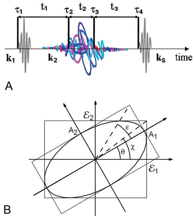
Phase, amplitude, and polarization pulse shaping. (A) Laser pulse sequence and time variables used in eqs 254 and 261 to describe a heterodyne-detected two-pulse 2D photon-echo experiment. (B) Polarization ellipse representation of the electric field (adapted from Brixner³²⁸). A₁ and A₂ are the major and minor principle axes that define the angle of ellipticity ε. The additional angles are the orientation angle of the ellipse θ and the auxiliary angle χ. The principal axes A₁ and A₂ are connected to the laboratory-frame amplitudes and by a principle-axis transformation. The polarization state of the laser pulses is defined by θ and ε. The sign of ε also defines the helicity: positive (negative) ε corresponds to the left (right) elliptically polarized light.

We consider a pulse propagating along z (eq 252) with two polarization components ν = x and y. The field will be described using the following variables. An auxiliary angle χ_j(t) ε [0, π/2] represents the ratio of the amplitudes (t):

$${\chi }_j(t)=arctan\frac{{\mathbb{E}}_{jy}(t)}{{\mathbb{E}}_{jx}(t)}.$$ (255)

A second angle δ_j(t) ε [-π, π] is given by the difference between the temporal phase modulations:

$${\delta }_j(t)={\varphi }_{jy}(t)-{\varphi }_{jx}(t),$$ (256)

θ̃_j(t) ε [-π/4, π/4] is a third angle

$${\stackrel{\sim }{\theta }}_j(t)=\frac{1}{2}arctan[tan(2{\chi }_j(t))cos{\delta }_j(t)].$$ (257)

The orientation angle of the ellipse θ _j(t) ε [-π/2, π/2] is then given by

$${\theta }_j(t)=\{\begin{array}{ll}{\stackrel{\sim }{\theta }}_j(t)\hfill & \text{if}{\chi }_j(t)\le \pi /4,\hfill \\ {\stackrel{\sim }{\theta }}_j(t)+\pi /2\hfill & \text{if}{\chi }_j(t)>\pi /4\wedge {\stackrel{\sim }{\theta }}_j(t)<0,\hfill \\ {\stackrel{\sim }{\theta }}_j(t)-\pi /2\hfill & \text{if}{\chi }_j(t)>\pi /4\wedge {\stackrel{\sim }{\theta }}_j(t)\ge 0.\hfill \end{array}$$

The ellipticity angle ε_j(t) ε [-π/4, π/4] is

$${\epsilon }_j(t)=\frac{1}{2}arcsin[sin(2{\chi }_j(t))sin{\delta }_j(t)].$$ (258)

Finally, the total phase ϕ_j(t) of the laser-field oscillation with respect to the perihelion of the momentary light ellipse is defined as

$${\varphi }_j(t)={\varphi }_{jx}(t)+\text{sign}[{\theta }_j(t){\epsilon }_j(t)]\times arccos\left[\sqrt{\frac{I_j(t)}{{[{\mathbb{E}}_{jx}(t)]}^2}}cos{\theta }_j(t)cos{\epsilon }_j(t)\right].$$ (259)

The instantaneous pulse frequency ω_j(t) is given by the time derivative of ϕ_j(t)

$${\omega }_j(t)={\overline{\omega }}_j+\frac{\text{d}{\varphi }_j(t)}{\text{d}t}.$$ (260)

Various porphyrin structures, such as dimers, rings, tapes, wheels, and boxes, have been proposed as potential artificial light-harvesting systems.^{4,96,97,279,329,330} The Soret band was described by the Frenkel-exciton model using known parameters.^263,331 Each porphyrin has two orthogonal electronic transitions (Figure 29A). The electronic level scheme consists of three manifolds: a ground state (g), four singly excited states (e), and six doubly excited states (f) (Figure 29B).

Figure 29.

Pulse shaping control of excitons in the Soret band of a chiral porphyrin dimer. (A) Structure of the complex. (B) The exciton level scheme: the ground state, four single-exciton states, and six two-exciton states. (C) and (D) are the linear absorption and circular dichroism (CD) spectra, respectively, which were obtained using the following parameters: the fluctuation magnitude Δ = 145 cm⁻¹ and the relaxation rate Λ = 160 cm⁻¹ at room temperature k_BT ) 207 cm⁻¹ (eq 169). (E) Absolute magnitudes of heterodyne-detected two-pulse 2D photon-echo spectra: xxxx and xyyx tensor components with unshaped Gaussian laser pulses; pure-polarization pulse shaping (P); shaping of polarization, spectral and temporal pulse profiles (STP). Arrows indicate the optimized peaks. (F) Quasi-3D electric-field representation of the P and STP laser pulses. The instantaneous frequencies are indicated by colors with an arbitrary color scheme where blue marks are for the center frequency ω₀. The projections to x (bottom) and y (top) axes represent the amplitude envelopes of the and components of the electric field (see ref 279).

We shall compare four laser pulse-shaping protocols. The first (ST_||) involves spectral and temporal shaping of both x- and y-components, creating parallel linearly polarized pulses. The real and imaginary components of the electric field are independently varied. The second form (ST_⊥) involves spectral and temporal shaping with perpendicular linearly polarized pulses. The third (P) involves pure-phase polarization pulse shaping constructed using the iterative Fourier transform (IFT) algorithm.^279,332 The temporal envelopes (t) and (t) are varied holding the total temporal intensity profile $I_j(t)={\mathbb{E}}_{jx}^2(t)+{\mathbb{E}}_{jy}^2(t)$ as well as the spectral amplitudes of both electric field components (ω) and $I_j(\omega )={\stackrel{\sim }{\mathbb{E}}}_{jx}^2(\omega )+{\stackrel{\sim }{\mathbb{E}}}_{jy}^2(\omega )$ fixed to the initial values. The temporal (ϕ_jv(t)) and spectral (ϕ̃jv(ω);) phases were calculated using the IFT algorithm. To obtain (t), we varied the auxiliary angle χ_j(t). The fourth (STP) is the most general and uses the entire parameter space involving spectral, temporal, and polarization pulse shaping.

We apply these pulse-shaping algorithms to control the amplification of weak spectral features in heterodyne-detected 2D two-pulse photon-echo (PE) signals with a Gaussian linearly polarized first pulse with wavevector k₁, local oscillator k_s pulse, and a second pulse k₂ = k3 (Figure 28A) tuned with adaptive pulse shaping. The signal is generated in the direction k_s = −k₁ + 2k₂ by varying t₁ and t₃ and holding t₂ = 0. The signals were calculated by performing multiple time integrations and taking Fourier transforms with respect to the time delays between the first and second laser pulses, τ, and between the second and the local oscillator pulse, t,⁵²

$$\begin{array}{l}{S}_{{\mathit{k}}_{\text{I}}}({\mathrm{\Omega }}_1,{\mathrm{\Omega }}_2)=\sum _{\alpha ,\beta ,\gamma ,\delta }{\int }_0^{\infty }{\int }_0^{\infty }\text{d}t\text{d}\tau {\text{e}}^{i{\mathrm{\Omega }}_1\tau +i{\mathrm{\Omega }}_{2}t}{\int }_0^{\infty }\text{d}{t}_3{\int }_0^{\infty }\text{d}{t}_2{\int }_0^{\infty }\text{d}{t}_1\times \\ R_{\delta \gamma \beta \alpha }^{(3)}(t_3,t_2,t_1){\text{e}}^{i(2{\omega }_2-{\omega }_1)t_3+i({\omega }_2-{\omega }_1)t_2-i{\omega }_1{t}_1}\times {\mathbb{E}}_{3\delta }^{\ast }(t){\mathbb{E}}_{2\gamma }(t-t_3){\mathbb{E}}_{2\beta }(t-t_3-t_2){\mathbb{E}}_{1\alpha }^{\ast }(t+\tau -t_3-t_2-t_1),\end{array}$$ (261)

where (t) are the complex laser pulse envelopes.

The simulated spectra are displayed in Figure 29E. The reference 2D PE spectrum obtained with two linearly polarized Gaussian pulses (top row) has two major diagonal peaks, D1 and D2, and weak off-diagonal peaks, C1 and C2. The major contributions to D1 and D2 are the one-exciton states at $\mathrm{\Delta }{\mathrm{\Omega }}_1^{\prime }$ and $\mathrm{\Delta }{\mathrm{\Omega }}_3^{\prime }$, respectively (Figure 29C). The chosen control target was to amplify the off-diagonal (C1 and C2) relative to the diagonal (D1 and D2) peaks. To specify the target, we define the integrated intensity of the jth peak.

$$I_j\equiv {\int }_{-\delta }^{\delta }\text{d}{\mathrm{\Omega }}_1{\int }_{-\delta }^{\delta }\text{d}{\mathrm{\Omega }}_2{S}_{{\mathit{k}}_{\text{I}}}({\mathrm{\Omega }}_1+{\mathrm{\Omega }}_1^j,{\mathrm{\Omega }}_2+{\mathrm{\Omega }}_2^j).$$ (262)

The ratios of the integrated diagonal and cross-peaks T₁ = (I_D1 + I_D2)/I_C1 and T₂ = (I_D1 + I_D2)/I_C2 were used as cost functions and minimized using a genetic algorithm (GA). The optimal 2D PE spectra P and STP are displayed in rows 2 and 3 of Figure 29E. Peaks D1, D2, C1, and C2 are marked by circles. Arrows mark the amplified target peaks.

Complete resolution and amplification of the target peaks was only achieved using the STP (target T₁) and STP′ (target T₂). The resulting polarization-shaped pulses are displayed using the quasi-3D electric-field representation based on specifying the temporal intensity I_j(t), total phase ϕ_j(t), orientation of the ellipse θ_j(t), and ellipticity ε_j(t).^305,328 In Figure 29F, we show these parameters as a set of instantaneous light ellipses at different times along the electric-field propagation axis. The ellipse sizes represent the intensity, and their shapes provide instantaneous snapshots of the polarization state. The projections represent the intensities of individual electric-field components. The variation of the total phase (chirp) is shown by color. Weak cross-peaks were enhanced compared to the intense diagonal peaks. The optimized electric fields with different polarizations select different Liouville space pathways of the tensor components of the response functions, highlighting several tensor elements with distinct features. It is clear by comparison of the four pulse-shaping strategies that modulation of the polarization profiles was necessary in order to achieve the complete resolution and amplification of the cross-peaks.⁹⁷

14.2. Adaptive Optimization of Pulse-Polarization Configurations

The multiparameter coherent-control schemes described above involve elaborate pulse-shaping and characterization techniques. We now describe a different approach for simplifying 2D spectra by taking linear combinations of various tensor components of the response function.

It was shown in section 13 that the third-order 2D signals depend on various tensor components of the response function ℝ_{ks;ν4ν3ν2ν1}.⁷⁹ The nonchiral (NC) tensor components (dipole approximation) include ν₄ν₃ν₂ν₁ ≡ xxyy, xyxy, and xyyx (note that xxxx = xxyy + xyxy + xyyx). We label them $T_1^{(\text{NC})}-T_3^{(\text{NC})}$. The nine linearly independent chirality-induced (CI) k_I = −k₁ + k₂ + k₃ response function tensor components are labeled $T_1^{(\text{CI})}-T_9^{(\text{CI})}$. These were defined in Tables 1–3 in section 13.

We have constructed the following superposition of linearly independent response function tensor components:

$${\mathbb{S}}^{(\text{NC}/\text{CI})}({\omega }_1,{\omega }_3)=\sum _{j=1}^n{c}_j{T}_j^{(\text{NC}/\text{CI})}$$ (263)

where n = 3 for the NC and n = 9 the CI techniques. The complex coefficients $c_i=c_i^{\prime }+i{c}_i^{″}$ were varied using a genetic algorithm in order to optimize the ratios of the amplitudes of selected peaks in the porphyrin dimer described above (Figure 29).²⁶³ The interference of CI tensor components was used to suppress the strong diagonal peaks and amplify weak cross-peaks (Figure 30). The initial nonchiral signals at delay time t₂ = 0 were simulated with a homogeneous broadening γ = 500 cm⁻¹. Only two diagonal peaks, P₁ and P₅, and two cross-peaks, P₂ and P₄, were resolved. In the chirality-induced T₁–T₉ spectra, the remaining four cross-peaks P₃, P₆, P₇, and P₈ were only partially resolved. Using a genetic algorithm, we found optimal linear combinations of CI tensor components that amplify these peaks and reveal information about couplings of the x- and y-polarized transitions. This information was not available from the absorption spectra or the initial 2D NC spectra. The Soret-band in porphyrin aggregates is the strongest and is connected with interesting photophysical processes such as S₂-exciton emission and dynamic intensity borrowing.³³³ The optimized cross-peaks provide additional information that is not revealed by superpositions of the nonchiral tensor components.

Figure 30.

Coherent control of 2D signals of a porphyrin dimer by a linear combination of 2D CI tensor components. Shown are absolute magnitude at delay time t₂ = 0: four nonchiral tensor components xxxx, xxyy = xyxy, xyyx; nine chirality-induced tensor components T₁–T₉; and optimized linear combinations P₃, P₆, P₇, and P₈, highlighting the initially poorly resolved cross-peaks with red, green, black, and blue circles, respectively. Optimized peaks are marked by arrows. The top left panel shows the xxxx signal calculated with narrow line width where all peaks are resolved.

We next demonstrate how coherent control may be applied to manipulate exciton-transport pathways²⁶² in the FMO complex as revealed by 2D experiments. The simulated xxxx spectrum shown in Figure 31 (left column) fits the experimental data.^40,80 Thin lines on both axes in the 2D spectra mark the exciton 1–7 positions in order of increasing energy. The cross-peaks (2,4) and (2,5) corresponding to exciton states 4 and 5 on the Ω₁-axis, and state 2 on the Ω₃-axis, overlap with the diagonal peaks of the same sign, forming an L-shape signal.

Figure 31.

Coherent control of energy transfer in FMO by adaptive optimization of a linear combination of 2D CI tensor components. Absolute magnitude of 2D signals: nonchiral xxxx and optimal 2D CI (fast) and (slow) linear combinations corresponding to the optimizations of the fast and slow energy-transfer pathways. The optimized cross-peaks (1, 5) and (1, 7) are indicated with red and green circles, respectively.

Using coherent control combined with a genetic learning algorithm, different energy-transfer channels were separated by optimizing a linear superposition of CI tensor components. The control targets were aimed at manipulating various peaks in these 2D spectra by selecting the ratios of the integrated cross-peaks in the absolute values of the 2D signals at long delay time t₂ = 5 ps. Two cross-peaks (1,5) and (1,7) contributing to predicted fast and slow pathways^40,80 are marked in Figure 31 by red and green circles, respectively. These cross-peaks represent energy transfer from higher to lower energy states, and grow as a function of t₂. The (1,7) cross-peak was not resolved in the xxxx spectrum.

In the optimization of the fast energy-transfer pathway, the ratio of (1,5) to (1,7) is maximized. The red circle and arrow mark the cross-peaks (1,5) and (1,2), respectively. The optimal coefficients obtained from the optimizations at t₂ = 5 ps were then used to obtain the 2D spectra for other t₂ delay times. The exciton states 1, 2, and 5 are involved in the fast pathway, and the corresponding cross-peaks are enhanced. For the slow pathway, the ratio of (1,7) to (1,5) is maximized. Green circle and arrow indicate cross-peaks (1,7) and (1,3), respectively. As a result, both pathways are separately optimized and well-resolved. In addition, the fast pathway shows a node (a region where the signal vanishes) between the arrow and the red circle, corresponding to the elimination of the (1,3) cross-peak. Similarly, in the optimization of the slow pathway, we see nodes corresponding to the elimination of the (1,2), (1,4), and (1,5) cross-peaks of the fast pathway. Optimal laser-pulse polarization configurations obtained using coherent control and genetic algorithms enhance the chirality-induced spectral features, revealing a specific energy-transfer pathway that was not resolved in the xxxx spectra. These methods may be applied to other 2D techniques. They have also been applied, for example, in vibrational 2D spectroscopy to resolve the structure of amyloid fibrils.³³⁴

In conclusion, pulse shaping combined with coherent control can increase the sensitivity of multidimensional spectroscopy of molecular aggregates by unraveling weak cross-peaks from otherwise congested spectra.

15. Discussion and Conclusions

Femtosecond nonlinear optical spectroscopy had gradually evolved from simple pump–probe (transient absorption) applications in the early 1980s to the elaborate coherent multidimensional techniques surveyed here. The field has been driven by both ultrafast pulse-laser source technology (down to attoseconds)²⁶⁸ and progress in the theoretical modeling of complex molecular assemblies with dissipation.

The response-function formalism provides a unified picture of nonlinear optical techniques in systems driven by moderately strong optical fields. The signals are given as convolutions of response functions to various orders in the incoming fields, with the field envelopes. The response functions carry all necessary molecular information for calculating the optical signals.

We have surveyed the key aspects of the theory, focusing on coherent third-order heterodyne-detected signals. This holographic phase-sensitive detection gives the signal field itself (both amplitude and phase). Early third-order optical measurements used homodyne detection, which only gives the signal intensity. For completeness, we briefly describe these signals using the response-function formalism.

The simplest third-order technique, pump–probe, is performed with two optical pulses with variable delay time τ. The first pulse, the pump, perturbs the system, and the second, the probe, detects the time evolution of this perturbation. The technique can be performed in various configurations: the pump and probe can have same/different carrier frequencies, have same/different bandwidths, and be in completely different optical regions ranging from THz to the UV. Instead of using the response function, this signal can be alternatively described as an induced absorption/emission events from a nonstationary state. Using the third-order response function when the pump and the probe are temporally well-separated, the pump is associated with the first two interactions, while the probe induces the third interaction and the self-heterodyned detection. Since the first two interactions occur within the pulse envelope and are indistinguishable, the signal is the sum of the k_I and k_II techniques, which only differ by the order of the first two interactions (Figures 4, 5). The delay time t₁ is controlled by the pump-field, while t₃ is controlled by the probe. The delay between pump and probe pulses then coincides with the time variable t₂. The pump–probe signal is thus given by

$$I_{\text{pp}}({\omega }_{\text{pr}},\tau ,{\omega }_{\text{pu}})=Im[S_{{\mathit{k}}_{\text{I}}}({\omega }_{\text{pr}},\tau ,-{\omega }_{\text{pu}})+S_{{\mathit{k}}_{\text{II}}}({\omega }_{\text{pr}},\tau ,{\omega }_{\text{pu}})],$$ (264)

where ω_pu and ω_pr are the pump and probe carrier frequencies. This gives the absorptive lineshape (eq 219).

Transient grating is another closely related technique. Here, two pump-pulses with wavevectors k₁ and k₂ are applied simultaneously; the probe comes after a delay τ and the homodyne signal is measured in the k₁ − k₂ + k_pr direction. Usually ω_pu and ω_pr are tuned to the same optical transition and the 1D time-domain signal is recorded versus τ. The pulse bandwidth selects the relevant spectral region. This homodyne signal is given by

$$I_{\text{TG}}(\tau ,{\omega }_{\text{pu}})={\int }_0^{\infty }\text{d}{t}_3{\mid S_{{\mathit{k}}_{\text{I}}}(t_3,\tau ,-{\omega }_{\text{pu}})+S_{{\mathit{k}}_{\text{II}}}(t_3,\tau ,{\omega }_{\text{pu}})\mid }^2.$$ (265)

Similar to the pump-probe, this signal monitors excited-state population and relaxation.

Finally, we note the three-pulse photon-echo peak-shifts (3PEPS) often used to study bath fluctuations. It uses three pulses with the same carrier frequency and a broad bandwidth. 3PEPS measures the homodyne k_I signal as a function of two delay times t₁ and t₂.

$$I_{3\text{PEPS}}(t_2,t_1)={\int }_0^{\infty }\text{d}{t}_3{\mid S_{{\mathit{k}}_{\text{I}}}(t_3,t_2,t_1)\mid }^2.$$ (266)

This signal is usually displayed as a family of 1D plots vs t₁, for various values of t₂. For an ensemble of two-level systems, the signal along t₁ grows for short t₁, reaches a maximum at t₁ = τ_M, and eventually decays. The value of τ_M and its dependence on t₂ reflects the bath correlation function (eq 343). Thus, the dependence τ_M(t₂) (the 3PEPS signal) reveals direct information on the system–bath couplings.^{42–44,48,335,336} This interpretation is limited to a single two-level chromophore.

We have introduced two types of response functions: one (R) connecting the induced polarization with the incoming electric fields (eq 14), and the other (ℝ) relates the induced current with the vector potential of the field (eq 238). The relation between them can be established using the Maxwell equations. In the dipole approximation where the signals calculated using both approaches must coin-cide, we find that R → (ω₁ω₂ω₃ω₄⁾⁻¹ℝ, where ω_j is the carrier frequency of the jth laser field. We derived R in the dipole approximation, ignoring the magnetic dipole and the electric quadrupole contributions. This is adequate for molecular complexes of nonchiral molecules. The response function R may be extended to include the magnetic corrections. However, it is much more convenient to calculate ℝ instead.

We have used the Frenkel-exciton model in the boson representation. Two types of parameters are responsible for the nonlinear optical signals. The quartic potential U_mnkl controls the exciton scattering when the field is turned off, while ${\mathit{\mu }}_m^{(2)}$ represents anharmonic system–field interaction. Hard-core bosons are a special case of this model, as shown in Appendix C. They have U_mmmm = ∞. This model developed here for electronic excitations also applies to vibrational excitations. We then model the excitations as intrinsically boson-like with a finite U_mmmm and ${\mathit{\mu }}_m^{(2)}=0$ (soft-core bosons). This approach has been applied to coupled vibrations in polypeptides.^67,100,337

The supermolecule and quasiparticle scattering are two conceptually different approaches for calculating the response functions of aggregates. The sources of nonlinearities in these descriptions look very different. In the supermolecular representation, the double-exciton states are included explicitly, and interband transitions do not follow a harmonic oscillator model. In the quasiparticle representation, the final expressions involve only single-exciton states. Double-exciton resonances are recovered from the frequency-dependent exciton-scattering matrix. The relation and equivalence of the two representations can be established when supermolecule double-exciton states are expanded in the single-exciton product basis for an isolated system. Differences remain since different approximations are made for the system–bath interaction.

In this review, the quasiparticle representation has been used in conjunction with simple Lorentzian line shapes in the Markovian limit. More elaborate line-shape theories could be developed (equivalent to the CGF or SLE); however, this is usually not necessary in large aggregates where the lineshapes are often controlled by inhomogeneities and spectral congestions. Each peak is then composed of many overlapping transitions. The detailed microscopic description of bath dynamics is crucial for small systems (~10 or less coupled oscillators), where the line shapes are better resolved.

The marriage of coherent-control pulse-shaping techniques with 2D spectroscopy offers numerous future possibilities. The rich information obtained through snapshots of electronic dynamics can then be further refined by manipulating the interference of various Liouville space pathways. These techniques may also be used to shift and isolate specific resonances, facilitating the assignment of electronic transitions.

Chirality-induced signals may lead to useful applications of multidimensional coherent spectroscopy to structure determination. X-ray crystallography and NMR determine structures of molecular complexes with atomic resolution. Optical spectroscopy can be used as a complimentary technique for further structure refinement.

Electronic nonlinear spectroscopy is most valuable for tracking dynamical events in molecules and their complexes. Unlike traditional 1D transient-absorption and transient-grating techniques, in multidimensional coherent techniques, a large amount of information is gathered in a single shot. Numerical data processing and analysis techniques need to be developed to help extract system information (e.g., Hamiltonian, bath, structural, and relaxation parameters) from the measured signals.

The various methods and techniques reviewed here are based on a generic exciton and supermolecule approaches within the RWA (sections 2, 5, 6) and may be applied to other frequency regimes: from THz to X-ray. 2D techniques, originally developed in NMR,⁵³ were extended during the past decade to IR laser spectroscopy.^60,338–343 Simulation protocols based on molecular dynamics (MD) strategies have been reviewed recently in ref 67. These applications use the same formalism; however, the vibrations are bosons. Electrostatic parametrization of vibrational Hamiltonian parameters is currently a useful technique for including fluctuations, simulated by MD trajectories. Developing electrostatic maps for electronic Hamiltonians is necessary for affordable modeling of solvation effects.

The theoretical apparatus presented in this review has been implemented in the computer software package “SPECTRON”, which has been used for simulating coherent nonlinear optical responses in IR,^{79,91,92,94,95,155,344,345} visible,^81,97 and UV^82,156 regions. The code includes the super-molecule and quasiparticle approaches as well as the spectral lineshape-broadening models described in sections 2, 4, 9, and 11.

Figure 33.

Feynman diagrams of the quasiparticle dynamics in k_II technique. The left-most diagram is for the μ⁽⁰⁾ = 0 case, while others include μ⁽⁰⁾ ≠ 0. The symbols are the same as in Figure 32.

Biographies

Darius Abramavicius was born in 1974 in Alytus, Lithuania. He received his M.S. degree from Vilnius University in 1998 and his Ph.D. degree under the supervision of Prof. Leonas Valkunas from the Institute of Physics at Vytautas Magnus University, Lithuania, in 2002. He then joined the group of Professor Shaul Mukamel at University of Rochester (New York, U.S.A.). He moved to the University of California Irvine in 2003. During 2005–2006, he was a temporary lecturer in Theoretical Physics Department of Vilnius University in Lithuania. Currently he is a visiting scientist at the University of California, Irvine, in the group of Prof. S. Mukamel. His research interests are in the field of optical and dynamical properties of molecular complexes.

Benoit Palmieri was born in 1978 in Montréal, Canada. He received his Ph.D. degree under the direction of Professor David Ronis from the chemistry department of McGill University in 2007. The main subject of his Ph.D. thesis was the theoretical study of diffusion of gas or liquid molecules inside channeled structures (zeolites). He joined the group of Professor Shaul Mukamel in 2007, where he worked on the nonlinear optical response of photosynthetic systems and on the importance of interband excitonic couplings. He is now working at the Canadian Space Agency under the direction of Dr. Marcus Dejmek, developing theoretical models of crystal growth.

Dmitri V. Voronine was born in 1979 in Moscow, Russia, and is currently a Postdoctoral Researcher in the group of Prof. Tobias Brixner at the Institut für Physikalische Chemie, Universität Würzburg, Germany. He received his Ph.D. in 2004 from the Center for Photochemical Sciences, Bowling Green State University, under the supervision of Prof. Michael A. J. Rodgers, and did postdoctoral work with Prof. Shaul Mukamel at the Department of Chemistry, University of California, Irvine. He has been the recipient of the McMaster Fellowship (BGSU) and the RCCM Excellent Young Investigator award (U. Würzburg). His research interests in theoretical and experimental physical chemistry and nanobiophysics include applying the methods of coherent control with laser pulse shaping to femtosecond 2D spectroscopy of complex systems such as biomolecules, photosynthetic complexes, chiral and fractal molecular aggregates, porphyrins and carotenoids; and ultrafast nano-optics of metal nanostructures for space-time-resolved spectroscopy with nanometer spatial and femtosecond temporal resolution.

František Šanda was born in 1976 in Domažlice, Czech Republic. He received his Ph.D. in Theoretical Physics (supervisor Vladislav Čápek) in 2003 from Charles University, Prague. From 2004 to 2005, he had a postdoctoral appointment at the University of California, Irvine, in the group of Prof. Shaul Mukamel. He is an Assistant Professor at Institute of Physics, Faculty of Mathematics and Physics, Charles University in Prague since 2006. His research interest focuses on stochastic modeling of dynamic processes in Liouville space, with emphasis on applications in spectroscopy.

Shaul Mukamel, currently the Chancellor Professor of Chemistry at the University of California, Irvine, received his Ph.D. in 1976 from Tel Aviv University. Following postdoctoral appointments at MIT and the University of California, Berkeley, he has held faculty positions at Rice University, the Weizmann Institute, and the University of Rochester. He is the recipient of the Sloan, Dreyfus, Guggenheim, and Alexander von Humboldt Senior Scientist award and the Lippincort Award and is a fellow of the American Physical Society and the Optical Society of America. His interests focus on developing computational techniques for the design of novel ultrafast laser pulse sequences for probing electronic and vibrational dynamics in molecules. Biophysical applications include folding and dynamical fluctuations in proteins and DNA, hydrogen bonding, long-range electron and energy transfer in photosynthetic complexes, and signatures of chirality. Other areas are attosecond x-ray spectroscopy, excitons in semiconductor nanostructures, many-body effects in quantum optics, and photon and electron statistics in single-molecule spectroscopy and open molecular junctions. He is the author of over 600 publications in scientific journals and the textbook, Principles of Nonlinear Optical Spectroscopy (Oxford University Press), 1995.

17. Appendix A: Survey of Linear Optical Techniques

Linear optical signals are generated by a single interaction with the incident optical field. Three types of linear signals are most widely used: absorption, where the transmission of the incident beam is measured; linear dichroism, the difference between two polarized absorptions (longitudinal, L, and transverse, T) in oriented samples; and circular dichroism, the difference between the absorptions of two circularly polarized beams (left, L, and right, R).

Using the response function formalism, the linear absorption may be interpreted as follows. The incident beam interacts once with the molecule and induces the linear polarization. This polarization then creates the outgoing optical field, which interferes with the incoming beam. This is a self-heterodyne detection. The detector measures the net optical field, which is attenuated by the interference. The mathematical formulation is very nicely described in the book by Loudon.¹¹⁷

The absorption of the field is defined by following the field intensity in the medium, which follows

$$I(z)=I_0(z)exp(-{\kappa }_{a}z).$$ (267)

The absorption coefficient κ_a is given by

$${\kappa }_a(\omega )=\frac{4\pi \omega }{n(\omega )c}Im[R^{(1)}(\omega )].$$ (268)

Here, n(ω) is the refractive index of the medium, and c is the speed of light. The macroscopic response function of an isotropic ensemble of identical absorbers is related to the microscopic single-molecule response function by a three-dimensional orientational averaging. Using the response function eq 13, we get for the absorption coefficient

$${\kappa }_a(\omega )\propto \omega \sum _e{\mid {\mathit{\mu }}_e\mid }^2\frac{{\gamma }_{eg}}{{(\omega -{\omega }_{eg})}^2+{\gamma }_{eg}^2}.$$ (269)

Assemblies of oriented molecules are described by their tensor properties. The response function eq 13 is a second-rank tensor with respect to system symmetry axis. Equation 13 then involves the following orientationally averaged product:

$$\langle ({\mathit{\mu }}_2·{\mathit{\nu }}_2)({\mathit{\mu }}_1·{\mathit{\nu }}_1)\rangle =\sum _{i,j,\alpha ,\beta =x,y,z}\langle T_{i\alpha }{T}_{j\beta }\rangle {\mathit{\nu }}_2^{\alpha }{\mathit{\nu }}_1^{\beta }{\mathit{\mu }}_2^i{\mathit{\mu }}_1^j.$$ (270)

Here, we introduced the transformation tensor from the molecular (μ^α) to the laboratory frame (μⁱ), μⁱ = Σ_αT_iαμ^α We assume that the molecules are oriented along z and take the molecular z-axis to coincide with the laboratory z-axis. Orientational averaging in the xy plane then amounts to rotating the molecular xy plane around the z-axis. This can be easily calculated since, in this case, only five elements of the transformation tensor are nonzero: T_xx = cos φ, T_xy = −sin φ, T_yx = -sin φ, T_yy = cos φ, and T_zz = 1, and the orientational averaging amounts to an integration over the rotation angle φ:

$$\begin{array}{l}\langle T_{i\alpha }{T}_{j\beta }\rangle \equiv {(2\pi )}^{-1}{\int }_0^{2\pi }\text{d}\phi T_{i\alpha }(\phi )T_{j\beta }(\phi )\\ =2^{-1}[2{\delta }_{iz}{\delta }_{\alpha z}{\delta }_{jz}{\delta }_{\beta z}+{\delta }_{i\alpha }{\zeta }_{iz}{\delta }_{j\beta }{\zeta }_{jz}+({\delta }_{jy}{\delta }_{\beta x}-{\delta }_{jx}{\delta }_{\beta y})({\delta }_{iy}{\delta }_{\alpha x}-{\delta }_{ix}{\delta }_{\alpha y})].\end{array}$$ (271)

Thus, when μ₂ = μ₁ =μ, we obtain the following possible field configurations. For ν₂ = ν₁= z:

$$\langle (\mathit{\mu }·\mathit{z})(\mathit{\mu }·\mathit{z})\rangle ={({\mathit{\mu }}^z)}^2$$ (272)

and for ν₂ = ν₁ = x (the same holds for y):

$$\langle (\mathit{\mu }·\mathit{x})(\mathit{\mu }·\mathit{x})\rangle =2^{-1}[{({\mathit{\mu }}^x)}^2+{({\mathit{\mu }}^y)}^2].$$ (273)

The linear dichroism (LD) technique measures the difference between the absorption of two perpendicularly polarized beams in an oriented sample. The LD signal vanishes in unoriented samples. For an oriented sample, it is given by

$${\kappa }_{\text{LD}}(\omega )={\kappa }_{\text{L}}(\omega )-{\kappa }_{\text{T}}(\omega ),$$ (274)

where κ_L is the longitudinal absorption given by eq 269 with the transition amplitude eq 272:

$${\kappa }_{\text{L}}=\omega \sum _e\frac{{({\mathit{\mu }}_e^z)}^2{\gamma }_{eg}}{{(\omega -{\omega }_{eg})}^2+{\gamma }_{eg}^2},$$ (275)

whereas κ_T is the transverse absorption (eq 269) together with eq 273:

$${\kappa }_{\text{T}}=\omega \sum _e\frac{{\gamma }_{eg}}{2}\frac{{({\mathit{\mu }}_e^x)}^2+{({\mathit{\mu }}_e^y)}^2}{{(\omega -{\omega }_{eg})}^2+{\gamma }_{eg}^2}.$$ (276)

Circular dichroism (CD) is a chirality-induced linear technique, involving two circularly polarized beams. A circularly polarized beam propagating along z is described by rotating unit electric vector:

$$\mathit{E}(t)=\frac{1}{2}(\mathit{x}\mp i\mathit{y})exp(\mathit{ikz}-i\omega t)+c.c.,$$ (277)

where “− (+)” sign corresponds to R(L) circular polarization.

Using the response function, we get the induced polarization generated by the R/L beam:

$${\mathit{P}}_{\text{R}/\text{L}}=(\mathit{x}\mp i\mathit{y})(R_{xx}^{(1)}(\omega )\mp {iR}_{xy}^{(1)}(\omega ))exp(\mathit{ikz}-i\omega t)+c.c.$$ (278)

The circular dichroism signal is commonly defined in terms of the ellipticity angle,

$$tan(\theta )=\frac{E_{\text{R}}-E_{\text{L}}}{E_{\text{R}}+E_{\text{L}}},$$ (279)

where E_R/L are the transmitted field amplitudes of the R and L beams given by eq 282. For very small angles, we use tan(θ) ≈ θ and get

$$\theta (\omega )=-\frac{Re{R}_{xy}^{(1)}}{Im{R}_{xx}^{(1)}}.$$ (280)

Instead of ellipticity angle, the molar ellipticity angle and the rotational strength are often used.⁹³

18. Appendix B: Homodyne-Detected versus Heterodyne-Detected Coherent Signals

The induced polarization serves as a source for the signal field, which is eventually detected. Several detection schemes are possible. Neglecting the magnetic response, the electric field and polarization satisfy the Maxwell equation:

$$\nabla \times \nabla \times \mathit{E}+\frac{1}{c^2}\frac{{\partial }^2\mathit{E}}{\partial t^2}=-\frac{4\pi }{c^2}\frac{{\partial }^2\mathit{P}}{\partial t^2}.$$ (281)

For transverse field and for pencil-shape sample geometry, it is possible to derive a simple relation between the emitted field envelope and the envelope of the induced polarization:

$$E_s(t)=\frac{2\pi i}{n({\omega }_s)}\frac{{\omega }_s}{c}l{P}_s(t)\text{sinc(}\mathrm{\Delta }\mathit{k}l/2\text{)exp(}i\mathrm{\Delta }\mathit{k}l/2\text{)},$$ (282)

where n(ω_s) is the dielectric constant at frequency ω_s, l is the interaction length, and Δ_k = k_s − u₁k₁ − u₂k₂ − u₃k₃ is the wavevector mismatch between the polarization and the optical field; sinc(x) = sin(x)/x. Thus, the strongest amplitude occurs at the phase-matching condition Δk =0. The other important conclusion is that the signal field is directly proportional to the polarization amplitude, but is π/2 out of phase because of the i factor.

Two detection schemes for the signal are most commonly employed. These are known as homodyne and heterodyne detection. In homodyne detection (HOD), the detector is placed at the phase-matching direction and measures the integrated intensity of the signal field, or counts photons. The field intensity is proportional to the absolute value of the signal field. Thus, the homodyne signal is given by

$$S^{(\text{HOD})}=\int \text{d}t{\mid {\mathit{P}}_s(t)\mid }^2.$$ (283)

An additional time-gating device can be introduced that filters the incoming signal in a given time window before it is detected by the homodyne technique. This time-gated ho-modyne (TGH) detected signal is given by

$$S^{(\text{TGH})}(t)={\mid {\mathit{P}}_s(t)\mid }^2.$$ (284)

In heterodyne detection (HET), an additional laser pulse (local oscillator, E_H) is applied in the direction of the signal field, E_S. It interferes with the signal, and the resulting field is then detected by homodyne detector. We thus get

$$S^{(\text{HET})}=\int \text{d}t{\mid {\mathit{E}}_s(t)+{\mathit{E}}_{\text{H}}(t)\mid }^2\propto 2Re({\mathit{E}}_{\text{H}}^{\ast }(t)·{\mathit{E}}_s(t))+{\mid {\mathit{E}}_{\text{H}}(t)\mid }^2+{\mid {\mathit{E}}_s(t)\mid }^2.$$ (285)

The local oscillator (second term) can be readily subtracted. The |E_s(t)|² term is typically weak since E_s ≪ E_H, and thus, the HET approach detects the signal amplitude

$$S^{(\text{HET})}(t)=2Re({\mathit{E}}_{\text{H}}^{\ast }(t)·{\mathit{E}}_s(t)).$$ (286)

This measurement can be repeated with varying phase of E_H to reveal the induced polarization P_s(t) using eq 282.

19. Appendix C: Bosonization Schemes for Frenkel Excitons

Transformations between fermion and boson representations widely used in many-body problems may be employed for describing excitations in semiconductors³⁴⁶–³⁵³ and molecular aggregates.⁹²,¹³⁶,¹³⁷,³⁵⁴,³⁵⁵

Consider molecular aggregates made of multilevel molecules. Molecule m has a set of transitions a from its ground state. Each transition acts as a two-level system, where the molecule can be either in the excited state a or the ground state. The molecule is now viewed as a collection of two-level systems. Within the space of a single excitation and double excitations, an aggregate made of such molecules is described by the Frenkel-exciton Hamiltonian

$${\widehat{H}}_0=\hslash \sum _{mn}\sum _{ab}{V}_{ma,nb}{\widehat{b}}_{ma}^{†}{\widehat{b}}_{nb}+\hslash \sum _{\mathit{mnkl}}\sum _{\mathit{abcd}}{W}_{ma,nb}^{kc,ld}{\widehat{b}}_{ma}^{†}{\widehat{b}}_{kc}^{†}{\widehat{b}}_{nb}{\widehat{b}}_{ld},$$ (287)

where m, n label different molecules and ${\widehat{b}}_{mb}^{†}$ is a bosonic ( $[{\widehat{b}}_{ma},{\widehat{b}}_{nb}^{†}]={\delta }_{mn}{\delta }_{ab}$) exciton creation operator on molecule m of transition a (this can be brought into the form of eq 57 by relabeling pairs ma, nb, kc and ld as single indices). V_ma,nb is the exciton resonant coupling term, and $W_{ma,nb}^{kc,ld}$ is the two-boson interaction potential. When W ≪ V (weak scattering regime), the excitations are soft-core bosons, where two particles have a small penalty (anharmonicity), when occupying the same state in the molecule. The requirement that two excitations cannot reside on the same molecule is satisfied by shifting the unphysical state energies out of the physical window of interest. In the Hamiltonian equation (eq 287), this is done by setting $W_{ma,mb}^{mc,md}\to \infty$. The electronic excitations now become hard-core bosons. Note that, by varying $W_{ma,mb}^{mc,md}$, we can continuously turn soft-core into hard-core bosons.

As a simple example, consider two-level molecules. The bosons do not scatter when they are on different molecules. To describe this model, we set $W_{m,m}^{m,m}\to \infty$ for all m (the indices a, b, c, and d are redundant for this model), while it is finite for all other index combinations and describes double-exciton binding energies. The exciton-scattering matrix for coupled two-level systems can be calculated by taking this limit in eq 325,

$${\mathrm{\Gamma }}_{mm,nn}(\omega )=-{[{\mathbb{G}}^{(0)}(\omega )]}_{mm,nn}^{-1},$$ (288)

where all other elements vanish. Note that it involves the inversion of ℕ × ℕ matrix ${\mathbb{G}}_{mm,nn}^{(0)}$ (all other elements are neglected). These are given by

$${\mathbb{G}}_{mm,nn}^{(0)}(\omega )=\sum _{e_2,e_1}\frac{{\psi }_{e_{1}m}{\psi }_{e_{2}m}{\psi }_{e_{1}n}{\psi }_{e_{2}n}}{\omega -{\epsilon }_{e_2}-{\epsilon }_{e_1}+i{\gamma }_{e_2}+i{\gamma }_{e_1}}.$$ (289)

The response is given by eqs 127–129 using the transformation to the single-exciton basis with eq 120. In some cases (for instance, in the MFA), the response functions diverge. The scattering matrix of Appendix H can then be used.

An alternative bosonization scheme is possible in some cases.¹³⁷ Consider a single anharmonic oscillator described by the Hamiltonian:

$${\widehat{H}}_0=\hslash \epsilon [{\widehat{B}}^{†}\widehat{B}+1/2],$$ (290)

where the eigenstate energy ladder consists of only d energy levels so that 〈 B̂^† B̂〉 = 0, 1, •••, d – 1. In this case, B̂ are not boson operators; their commutation relations are as follows:

$$[\widehat{B},{\widehat{B}}^{†}]=1-\frac{d}{(d-1)!}{({\widehat{B}}^{†})}^{d-1}{\widehat{B}}^{d-1};{({\widehat{B}}^{†})}^d={\widehat{B}}^d=0,$$ (291)

The system thus behaves as harmonic only for low excitation levels: ${\widehat{B}}^{†}\mid j\rangle =\sqrt{(j+1)}\mid j+1\rangle$ when j < d; the higher-energy states do not exist.

This system can de described in terms of boson operators [b̂, b̂^†] = 1 using the following transformation,

$${\widehat{B}}^{†}=\sum _{n=0}^{\infty }\sum _{k=0}^{d-2}\frac{\sqrt{k+1}}{(dn+k)!\sqrt{dn+k+1}}{({\widehat{b}}^{†})}^{dn+k+1}\widehat{Z}{(\widehat{b})}^{dn+k},$$ (292)

and

$$\widehat{B}=\sum _{n=0}^{\infty }\sum _{k=0}^{d-2}\frac{\sqrt{k+1}}{(dn+k)!\sqrt{dn+k+1}}{({\widehat{b}}^{†})}^{dn+k}\widehat{Z}{(\widehat{b})}^{dn+k+1},$$ (293)

where Ẑ = exp(− b̂^† b̂).

This transformation can be extended for a system of coupled truncated oscillators described by the Hamiltonian (the zero-point energy (1/2 in eq 290) is ignored),

$${\widehat{H}}_0=\hslash \sum _n{\epsilon }_n{\widehat{B}}_n^{†}{\widehat{B}}_n+\hslash \sum _{mn}^{m\ne n}{J}_{mn}{\widehat{B}}_m^{†}{\widehat{B}}_n+\hslash \sum _{\mathit{mnkl}}{U}_{mn,kl}{\widehat{B}}_m^{†}{\widehat{B}}_n^{†}{\widehat{B}}_k{\widehat{B}}_l+\dots ,$$ (294)

where the operators B B̂ _m refer to the mth molecule and satisfy the commutation rules:

$$[{\widehat{B}}_n,{\widehat{B}}_m^{†}]={\delta }_{mn}\left(1-\frac{d}{(d-1)!}{({\widehat{B}}_m^{†})}^{d-1}{\widehat{B}}_m^{d-1}\right).$$ (295)

The bosonization transformation is then similar to eqs 292 and 293, but each operator has an additional index m. The resulting new Hamiltonian will be given in terms of various products of ${\widehat{b}}_m^{†}$ and b̂_m

As an example, consider a molecular aggregate of two-level molecules. The commutation relations (d = 2 in eq 295, hard-core bosons) are¹³⁶,³⁵³,³⁵⁴

$$[{\widehat{B}}_n,{\widehat{B}}_m^{†}]={\delta }_{mn}(1-2{\widehat{B}}_m^{†}{\widehat{B}}_m).$$ (296)

In third-order spectroscopy, it is sufficient to consider up to three-particle operators; all terms involving four or more creation and annihilation operators contribute only to higher orders in the field and can be neglected. It is, therefore, sufficient to consider the Frenkel-exciton Hamiltonian of the form

$${\widehat{H}}_0=\hslash \sum _{mn}{h}_{mn}{\widehat{B}}_m^{†}{\widehat{B}}_n+\hslash \sum _{\mathit{mnkl}}{U}_{mn,kl}{\widehat{B}}_m^{†}{\widehat{B}}_n^{†}{\widehat{B}}_k{\widehat{B}}_l.$$ (297)

For the dipole operator, we have

$$\widehat{\mathit{\mu }}=\sum _m{\mathit{\mu }}_m{\widehat{B}}_m+h.c.$$ (298)

The transformation eqs 292 and 293 within the single and double excitons reduce to

$${\widehat{B}}_m^{†}\approx {\widehat{b}}_m^{†}-{\widehat{b}}_m^{†2}{\widehat{b}}_m,$$ (299)

$${\widehat{B}}_m\approx {\widehat{b}}_m-{\widehat{b}}_m^{†}{\widehat{b}}_m^2.$$ (300)

The first term in the transformation is the single-exciton term, while the second term describes the Pauli exclusion. By substituting eqs 299 and 300 into eq 297, we get the transformed Hamiltonian,

$${\widehat{H}}_0=\hslash \sum _{mn}{h}_{mn}{\widehat{b}}_m^{†}{\widehat{b}}_n+\hslash \sum _{\mathit{mnkl}}{u}_{mn,kl}{\widehat{b}}_m^{†}{\widehat{b}}_n^{†}{\widehat{b}}_k{\widehat{b}}_l,$$ (301)

where u_mn,kl = −h_ml(δ_mnδ_nk + δ_nkδ_kl) + U_mn,kl. For the dipole operator, we similarly get

$$\mathit{\mu }=\sum _m{\mathit{\mu }}_m({\widehat{b}}_m-{\widehat{b}}_m^{†}{{\widehat{b}}_m}^2)+h.c.$$ (302)

We thus find ${\mathit{\mu }}_m^{(2)}=-{\mathit{\mu }}_m$ in this case (see eq 59 in ${\mathit{\mu }}_m^{(2)}$).

20. Appendix D: Contributions of Dipole-Operator Nonlinearity to the Third-Order Response Function

In this section, we generalize eqs 115–117 to include μ⁽²⁾ contributions to the response function. In the NEE, this corresponds to several new sources to the third-order polarization, whose contributions are visualized in the diagrams shown in Figures 32–34. The left-most diagram in each figure represents the contributions coming solely from μ as given in the main text (eqs 115–117). Various configurations of interactions with μ⁽²⁾ are shown in the other diagrams.

Figure 32.

Feynman diagrams for quasiparticle dynamics in the k_I technique. The left-most diagram is for μ⁽⁰⁾ = 0 case, while others include μ⁽⁰⁾ ≠0. Each interaction with the field is displayed by a solid dot. Time propagation is from the bottom up. The single solid line represents G(t) propagation, the double line is either (when both lines point to the same direction) or (when the lines point to opposite directions), and the triple line represents . Interaction with μ⁽⁰⁾ ≠ 0 is represented by a dot, where three lines meet. The response function for each contribution can be directly written from these diagrams.

Figure 34.

Feynman diagrams of the quasiparticle dynamics in k_III technique. The left-most diagram is for the μ⁽⁰⁾ = 0 case, while others include μ⁽⁰⁾ ≠ 0. The symbols are the same as in Figure 32.

The rules for these diagrams are as follows: vertical lines represent exciton propagators. As in the main text, a single line represents G, a double line stands for (both lines pointing up) or (lines pointing up and down), whereas a triple line represents . Solid dots represent μinteractions with the field, while red-circled dots represent μ⁽²⁾ interactions. Since μ⁽²⁾ is a local chromophore property in real space, all Green’s functions must converge into one point where the interaction takes place. The horizontal dashed line represents V. It also introduces an integral over the t₃ interval.

Using these rules, we obtain the following additional contributions to eq 115 for the response function for k_I:

$$R_{{\mathit{k}}_{\text{I}}}^{({\text{QP}}_2)}(t_3,t_2,t_1)=2i{\left(\frac{i}{\hslash }\right)}^3{\mathit{\mu }}_{n_4}^{\ast }{\mathit{\mu }}_{n_3}^{(2)}{\mathit{\mu }}_{n_2}{\mathit{\mu }}_{n_1}^{\ast }\times {\int }_0^{t_3}\text{d}{t}^{\prime }{G}_{n_4{n}_4^{\prime }}(t^{\prime })V_{n_4^{\prime }{n}_1^{\prime },n_3^{\prime }{n}_2^{\prime }}\times {\mathbb{G}}_{n_1^{\prime }{n}_3^{\prime }{n}_2^{\prime },n_1^{″}{n}_3{n}_3}^{(Z)}(t_3-t^{\prime }){\mathbb{G}}_{n_3{n}_1^{″},n_2{n}_1^{‴}}^{(N)}(t_2)G_{n_1^{‴}{n}_1}^{\ast }(t_1),$$ (303)

$$R_{{\mathit{k}}_{\text{I}}}^{({\text{QP}}_3)}(t_3,t_2,t_1)=2i{\left(\frac{i}{\hslash }\right)}^3{\mathit{\mu }}_{n_4}^{(2)\ast }{\mathit{\mu }}_{n_3}{\mathit{\mu }}_{n_2}{\mathit{\mu }}_{n_1}^{\ast }\times {\mathbb{G}}_{n_4{n}_4{n}_4,n_1^{″}{n}_2^{″}{n}_3}^{(Z)}(t_3){\mathbb{G}}_{n_2^{″}{n}_1^{″},n_2{n}_1^{‴}}^{(N)}(t_2)G_{n_1^{‴}{n}_1}^{\ast }(t_1),$$ (304)

$$R_{{\mathit{k}}_{\text{I}}}^{({\text{QP}}_4)}(t_3,t_2,t_1)=2i{\left(\frac{i}{\hslash }\right)}^3{\mathit{\mu }}_{n_4}^{(2)\ast }{\mathit{\mu }}_{n_3}^{(2)}{\mathit{\mu }}_{n_2}{\mathit{\mu }}_{n_1}^{\ast }\times {\mathbb{G}}_{n_4{n}_4{n}_4,n_1^{″}{n}_3{n}_3}^{(Z)}(t_3){\mathbb{G}}_{n_3{n}_1^{″},n_2{n}_1^{‴}}^{(N)}(t_2)G_{n_1^{‴}{n}_1}^{\ast }(t_1),$$ (305)

$$R_{{\mathit{k}}_{\text{I}}}^{({\text{QP}}_5)}(t_3,t_2,t_1)=2i{\left(\frac{i}{\hslash }\right)}^3{\mathit{\mu }}_{n_4}^{\ast }{\mathit{\mu }}_{n_3}^{(2)}{\mathit{\mu }}_{n_2}{\mathit{\mu }}_{n_1}^{\ast }\times G_{n_4{n}_3}(t_3){\mathbb{G}}_{n_3{n}_3,n_2{n}_1^{‴}}^{(N)}(t_2)G_{n_1^{‴}{n}_1}^{\ast }(t_1).$$ (306)

Note that, for two-level molecules when ${\mathit{\mu }}_n=-{\mathit{\mu }}_n^{(2)}$, eq 303 cancels some contributions from eq 115 and eq 304 cancels eq 305.

For k_II additional to eq 116, we similarly have

$$R_{{\mathit{k}}_{\text{II}}}^{({\text{QP}}_2)}(t_3,t_2,t_1)=2i{\left(\frac{i}{\hslash }\right)}^3{\mathit{\mu }}_{n_4}^{\ast }{\mathit{\mu }}_{n_3}^{(2)}{\mathit{\mu }}_{n_2}^{\ast }{\mathit{\mu }}_{n_1}\times {\int }_0^{t_3}\text{d}{t}^{\prime }{G}_{n_4{n}_4^{\prime }}(t^{\prime })V_{n_4^{\prime }{n}_2^{\prime },n_3^{\prime }{n}_1^{\prime }}\times {\mathbb{G}}_{n_2^{\prime }{n}_3^{\prime }{n}_1^{\prime },n_2^{″}{n}_3{n}_3}^{(Z)}(t_3-t^{\prime }){\mathbb{G}}_{n_3{n}_2^{″},n_1^{″}{n}_2}^{(N)}(t_2)G_{n_1^{″}{n}_1}(t_1),$$ (307)

$$R_{{\mathit{k}}_{\text{II}}}^{({\text{QP}}_3)}(t_3,t_2,t_1)=2i{\left(\frac{i}{\hslash }\right)}^3{\mathit{\mu }}_{n_4}^{(2)\ast }{\mathit{\mu }}_{n_3}{\mathit{\mu }}_{n_2}^{\ast }{\mathit{\mu }}_{n_1}\times {\mathbb{G}}_{n_4{n}_4{n}_4,n_2^{\prime }{n}_1^{\prime }{n}_3}^{(Z)}(t_3){\mathbb{G}}_{n_1^{\prime }{n}_2^{\prime },n_1^{″}{n}_2}^{(N)}(t_2)G_{n_1^{″}{n}_1}(t_1),$$ (308)

$$R_{{\mathit{k}}_{\text{II}}}^{({\text{QP}}_4)}(t_3,t_2,t_1)=2i{\left(\frac{i}{\hslash }\right)}^3{\mathit{\mu }}_{n_4}^{(2)\ast }{\mathit{\mu }}_{n_3}^{(2)}{\mathit{\mu }}_{n_2}^{\ast }{\mathit{\mu }}_{n_1}\times {\mathbb{G}}_{n_4{n}_4{n}_4,n_2^{\prime }{n}_3{n}_3}^{(Z)}(t_3){\mathbb{G}}_{n_3{n}_2^{\prime },n_1^{‴}{n}_2}^{(N)}(t_2)G_{n_1^{‴}{n}_1}(t_1),$$ (309)

$$R_{{\mathit{k}}_{\text{II}}}^{({\text{QP}}_5)}(t_3,t_2,t_1)=2i{\left(\frac{i}{\hslash }\right)}^3{\mathit{\mu }}_{n_4}^{\ast }{\mathit{\mu }}_{n_3}^{(2)}{\mathit{\mu }}_{n_2}^{\ast }{\mathit{\mu }}_{n_1}\times G_{n_4{n}_3}(t_3){\mathbb{G}}_{n_3{n}_3,n_1^{‴}{n}_2}^{(N)}(t_2)G_{n_1^{‴}{n}_1}(t_1).$$ (310)

For k_III, we have the following additional contributions to eq 117:

$$R_{{\mathit{k}}_{\text{III}}}^{({\text{QP}}_2)}(t_3,t_2,t_1)=2i{\left(\frac{i}{\hslash }\right)}^3{\mathit{\mu }}_{n_4}^{\ast }{\mathit{\mu }}_{n_3}^{\ast }{\mathit{\mu }}_{n_2}^{(2)}{\mathit{\mu }}_{n_1}\times {\int }_0^{t_3}\text{d}{t}^{\prime }{G}_{n_4{n}_4^{\prime }}(t^{\prime })V_{n_4^{\prime }{n}_3^{\prime }{n}_2^{\prime }{n}_1^{\prime }}\times {\mathbb{G}}_{n_3^{\prime }{n}_2^{\prime }{n}_1^{\prime },n_3{n}_2^{″}{n}_1^{″}}^{(Z)}(t_3-t^{\prime }){\mathbb{G}}_{n_2^{″}{n}_1^{″},n_2{n}_2}(t_2)G_{n_2{n}_1}(t_1),$$ (311)

$$R_{{\mathit{k}}_{\text{III}}}^{({\text{QP}}_3)}(t_3,t_2,t_1)=2i{\left(\frac{i}{\hslash }\right)}^3{\mathit{\mu }}_{n_4}^{(2)\ast }{\mathit{\mu }}_{n_3}^{\ast }{\mathit{\mu }}_{n_2}{\mathit{\mu }}_{n_1}\times {\mathbb{G}}_{n_4{n}_4{n}_4,n_3{n}_2^{\prime }{n}_1^{\prime }}^{(Z)}(t_3){\mathbb{G}}_{n_2^{\prime }{n}_1^{\prime },n_2{n}_1^{″}}(t_2)G_{n_1^{″}{n}_1}(t_1),$$ (312)

$$R_{{\mathit{k}}_{\text{III}}}^{({\text{QP}}_4)}(t_3,t_2,t_1)=2i{\left(\frac{i}{\hslash }\right)}^3{\mathit{\mu }}_{n_4}^{(2)\ast }{\mathit{\mu }}_{n_3}^{\ast }{\mathit{\mu }}_{n_2}^{(2)}{\mathit{\mu }}_{n_1}\times {\mathbb{G}}_{n_4{n}_4{n}_4,n_3{n}_2^{″}{n}_1^{″}}^{(Z)}(t_3){\mathbb{G}}_{n_2^{″}{n}_1^{″},n_2{n}_2}(t_2)G_{n_2{n}_1}(t_1),$$ (313)

$$R_{{\mathit{k}}_{\text{III}}}^{({\text{QP}}_5)}(t_3,t_2,t_1)=2i{\left(\frac{i}{\hslash }\right)}^3{\mathit{\mu }}_{n_4}^{\ast }{\mathit{\mu }}_{n_3}^{(2)\ast }{\mathit{\mu }}_{n_2}^{(2)}{\mathit{\mu }}_{n_1}\times G_{n_4{n}_3}(t_3){\mathbb{G}}_{n_3{n}_3,n_2{n}_2}(t_2)G_{n_2{n}_1}(t_1),$$ (314)

$$R_{{\mathit{k}}_{\text{III}}}^{({\text{QP}}_6)}(t_3,t_2,t_1)=2i{\left(\frac{i}{\hslash }\right)}^3{\mathit{\mu }}_{n_4}^{\ast }{\mathit{\mu }}_{n_3}^{(2)\ast }{\mathit{\mu }}_{n_2}{\mathit{\mu }}_{n_1}\times G_{n_4{n}_3}(t_3){\mathbb{G}}_{n_3{n}_3,n_1^{\prime }{n}_2}(t_2)G_{n_1^{\prime }{n}_1}(t_1).$$ (315)

21. Appendix E: Coherent Single- And Two-Exciton Green’s Functions: The Bethe Salpeter Equation

In this section, we describe the coherent exciton dynamics in the absence of the bath and the field. The single-exciton dynamics is described by the Green’s function G(t) by definition B(t) = G(t)B(0) and is a solution of eq 73. We introduce the frequency-domain Green’s functions:

$$G(\omega )=-i\int \text{d}tG(t)exp(i\omega t)$$ (316)

with the inverse transform

$$G(t)=i\int \frac{\text{d}\omega }{2\pi }G(\omega )exp(-i\omega t).$$ (317)

This gives, for single-exciton dynamics,

$$G(\omega )={(\omega -h+i\eta )}^{-1},$$ (318)

where η→ +0 guarantees causality. The double-exciton dynamics is described by Green’s function given by eq 84. In the frequency domain, we then get

$$\mathbb{G}(\omega )={(\omega -h^{(Y)}+i\eta )}^{-1}.$$ (319)

We next describe the two-exciton propagation in terms of single-exciton scattering. For this, we use h^(Y) = h⁽⁰⁾ + V, which gives

$$h_{mn,m^{\prime }{n}^{\prime }}^{(0)}=h_{m{m}^{\prime }}{\delta }_{n{n}^{\prime }}+h_{n{n}^{\prime }}{\delta }_{m{m}^{\prime }}$$ (320)

and we define a Green’s function with respect to h⁽⁰⁾

$${\mathbb{G}}^{(0)}(\omega )={(\omega -h^{(0)}+i\eta )}^{-1}.$$ (321)

The two-exciton Green’s function can be written as

$$\mathbb{G}(\omega )={(\omega -h^{(0)}-V+i\eta )}^{-1}.$$ (322)

Using the operator identity Â⁻¹ = B̂ ⁻¹ + B̂ ⁻¹(B̂ –  )  ⁻¹ and taking  = ω − h^(Y) + iη and B̂ = ω − h⁽⁰⁾ + iη, we obtain B̂ –  = VandarriveattheDysonequation:⁶⁸,⁷⁹,¹⁰⁴,¹⁰⁸,³²⁶

$$\mathbb{G}(\omega )={\mathbb{G}}^{(0)}(\omega )+{\mathbb{G}}^{(0)}(\omega )V\mathbb{G}(\omega ).$$ (323)

We next define the boson-scattering matrix Γ(ω) by the equation

$$V\mathbb{G}(\omega )=\mathrm{\Gamma }(\omega ){\mathbb{G}}^{(0)}(\omega ).$$ (324)

Combining eqs 323 and 324 gives

$$\mathrm{\Gamma }(\omega )={[1-V{\mathbb{G}}^{(0)}(\omega )]}^{-1}V.$$ (325)

Γ, like V, is short-range, making it computationally tractable. Substituting eq 324 into eq 323 and transforming back to the time domain, we obtain the Bethe Salpeter equation

$${\mathbb{G}}_{mn,kl}(t)={\mathbb{G}}_{mn,kl}^{(0)}(t)-{\int }_0^t\text{d}{t}_2{\int }_0^{t_2}\text{d}{t}_1\times \sum _{m^{\prime }{n}^{\prime }{k}^{\prime }{l}^{\prime }}{\mathbb{G}}_{mn,m^{\prime }{n}^{\prime }}^{(0)}(t-t_2){\mathrm{\Gamma }}_{m^{\prime }{n}^{\prime }{k}^{\prime }{l}^{\prime }}(t_2-t_1)G_{k^{\prime }{l}^{\prime },kl}^{(0)}(t_1),$$ (326)

where the first term, (t), is the free-exciton propagator, with matrix elements ${\mathbb{G}}_{nm,n^{\prime }{m}^{\prime }}^{(0)}(t)=G_{n{n}^{\prime }}(t)G_{m{m}^{\prime }}(t)$. The second term represents the contribution of exciton scattering. We note that the scattering matrix has different units than the Green’s function: in the frequency domain, G has dimensions of time, while Γ has dimensions of angular frequency; in the time domain, G(t) is dimensionless, while Γ(t) has units of frequency squared.

Equation 326 recasts the two-exciton evolution in terms of the free quasi-particle dynamics and their scattering in real space. A doubly excited state in this representation is described by two quasi-particles residing on the same site. Thus, the quasiparticle picture applies even for a single chromophore (ℕ= 1): two particles are then restricted to be on the same site, and their scattering appears as the diagonal anharmonicity, Δ_m.

For two-level chromophores, two excitons cannot reside on the same site. These are, therefore, known as hard-core bosons. By assuming that U couplings vanish, the hard-core boson scattering matrix is obtained from the boson-scattering matrix in the limit U_mm,mm → ∞. The scattering matrix is then given by ${\mathrm{\Gamma }}_{mm,nn}^{\text{HC}}(\omega )=-{[{\mathbb{G}}_{mm,nn}^{(0)}(\omega )]}^{-1}$ with all other elements vanishing. More complicated expression for the scattering matrix (eq 369) can be obtained for hard-core bosons without performing bosonization as in Appendix H (we then also have ${\mathit{\mu }}_n^{(2)}=-{\mathit{\mu }}_n$ coming from Pauli blocking).

Note that, in the MFA limit for the response functions in eqs 81–83, the response can be recast in the form of eqs 89–91 using the scattering matrix, ${\mathrm{\Gamma }}_{n_4{n}_3,n_2{n}_1}^{\mathit{MFA}}(\tau )=i\delta (\tau )V_{n_4{n}_3,n_2{n}_1}$ or in the frequency domain,

$${\mathrm{\Gamma }}^{\text{MFA}}(\omega )=V.$$ (327)

Comparing this with eq 323 shows that the MFA scattering matrix corresponds to the first-order correction of the two-exciton Green’s function (eq 323) in the scattering potential V. In the frequency domain, Γ^MFA(ω) = V, and we can write

$${\mathbb{G}}^{\text{MFA}}(\omega )={\mathbb{G}}^{(0)}(\omega )+{\mathbb{G}}^{(0)}(\omega )V{\mathbb{G}}^{(0)}(\omega ).$$ (328)

22. Appendix F: Real Space Description of Exciton Dephasing and Transport

In this section, we derive the dephasing matrices of the NEE given by eqs 99–102. For this purpose, we consider the case where the optical field is switched off.

The system and the bath are described by eqs 99–102. The exciton dynamics is described by the Heisenberg equation of motion as in section 6. However, because of the bath, the equations for the exciton variables will be coupled with the bath variables. The bath contributions are calculated perturbatively to second order in the system–bath coupling, where averages of bath and exciton variables can be factorized as $\langle {\widehat{B}}_n^{†}\dots {\widehat{B}}_1^{†}{B}_m\dots {\widehat{B}}_1{\widehat{a}}^{†}\widehat{a}\rangle =\langle {\widehat{B}}_n^{†}\dots {\widehat{B}}_1^{†}{B}_m\dots {\widehat{B}}_1\rangle \langle {\widehat{a}}^{†}\widehat{a}\rangle$.¹⁰⁷ For a harmonic bath at thermal equilibrium, we have

$$\langle {\widehat{a}}_{\alpha }^{†}{\widehat{a}}_{\beta }\rangle ={\delta }_{\alpha \beta }\widehat{n}(w_{\alpha }),$$ (329)

where

$$\overline{n}(\omega )=\frac{1}{2}[coth(\beta \hslash \omega /2)-1],$$ (330)

is the mean boson occupation number at temperature T and β = (k_BT)⁻¹. Using this factorization, we arrive at the following NEE:

$$i\frac{\text{d}}{\text{d}t}{B}_m=\sum _{m^{\prime }}{h}_{m{m}^{\prime }}{B}_{m^{\prime }}+\sum _{m^{\prime }kl}{V}_{m{m}^{\prime },kl}{Z}_{m^{\prime }kl}+{\stackrel{.}{\overline{B}}}_m,$$ (331)

$$i\frac{\text{d}}{\text{d}t}{Y}_{mn}=\sum _{m^{\prime }{n}^{\prime }}{h}_{mn,m^{\prime }{n}^{\prime }}^{(Y)}{Y}_{m^{\prime }{n}^{\prime }}+{\stackrel{.}{\overline{Y}}}_{mn},$$ (332)

$$i\frac{\text{d}}{\text{d}t}{N}_{mn}=\sum _k[h_{nk}{N}_{mk}-h_{mk}{N}_{kn}]+{\stackrel{.}{\overline{N}}}_{mn},$$ (333)

$$i\frac{\text{d}}{\text{d}t}{Z}_{\mathit{kmn}}=\sum _{m^{\prime }{n}^{\prime }}{h}_{mn,m^{\prime }{n}^{\prime }}^{(Y)}{Z}_{k{m}^{\prime }{n}^{\prime }}-\sum _{k^{\prime }}{h}_{k^{\prime }k}{Z}_{k^{\prime }mn}+{\stackrel{.}{\overline{Z}}}_{\mathit{kmn}}.$$ (334)

We start with the single-exciton dynamics B⁽¹⁾ described by eq 331 and neglecting the Z variable. The bath-related term in the equation of single-exciton variables is as follows:

$${\stackrel{.}{\overline{B}}}_m^{(1)}=\sum _n\sum _{\alpha }{d}_{mn,\alpha }(\langle {\widehat{B}}_n^{(1)}{\widehat{a}}_{\alpha }^{†}\rangle +\langle {\widehat{B}}_n^{(1)}{\widehat{a}}_{\alpha }\rangle ).$$ (335)

The Heisenberg equation of motion for bath-assisted variables $\langle {\widehat{B}}^{(1)}{\widehat{a}}_{\alpha }^{†}\rangle$ and 〈B̂⁽¹⁾â_α〉 reads

$$i\frac{\text{d}}{\text{d}t}\langle {\widehat{B}}_m^{(1)}{\widehat{a}}_{\alpha }\rangle =\sum _n{h}_{mn}\langle {\widehat{B}}_n^{(1)}{\widehat{a}}_{\alpha }\rangle +w_a\langle {\widehat{B}}_m^{(1)}{\widehat{a}}_{\alpha }\rangle +\sum _n{d}_{mn,\alpha }{B}_n^{(1)}(1+\langle {\widehat{a}}_{\alpha }^{†}{\widehat{a}}_{\alpha }\rangle ),$$ (336)

$$i\frac{\text{d}}{\text{d}t}\langle {\widehat{B}}_m^{(1)}{\widehat{a}}_{\alpha }^{†}\rangle =\sum _n{h}_{mn}\langle {\widehat{B}}_n^{(1)}{\widehat{a}}_{\alpha }^{†}\rangle -w_a\langle {\widehat{B}}_m^{(1)}{\widehat{a}}_{\alpha }^{†}\rangle +\sum _n{d}_{mn,\alpha }{B}_m^{(1)}\langle {\widehat{a}}_{\alpha }^{†}{\widehat{a}}_{\alpha }\rangle .$$ (337)

A formal solution of these equations gives the following:

$$\langle {\widehat{B}}_m^{(1)}{\widehat{a}}_{\alpha }\rangle (t)=-i{\int }_{-\infty }^t\text{d}\tau \sum _{n{n}^{\prime }}{G}_{mn}^{(c)}(t-\tau ){\text{e}}^{-i{w}_{\alpha }(t-\tau )}\times d_{n{n}^{\prime },\alpha }(1+\langle {\widehat{a}}_{\alpha }^{†}{\widehat{a}}_{\alpha }\rangle )B_{n^{\prime }}^{(1)}(\tau )$$ (338)

$$\langle {\widehat{B}}_m^{(1)}{\widehat{a}}_{\alpha }^{†}\rangle (t)=-i{\int }_{-\infty }^t\text{d}\tau \sum _{n{n}^{\prime }}{G}_{mn}^{(c)}(t-\tau ){\text{e}}^{i{w}_{\alpha }(t-\tau )}\times d_{n{n}^{\prime },\alpha }\langle {\widehat{a}}_{\alpha }^{†}{\widehat{a}}_{\alpha }\rangle )B_{n^{\prime }}^{(1)}(\tau ),$$ (339)

and where G^(c)(t) = θ(t) exp(−iht), where h is the matrix and h_mn is the zero-order Green’s function corresponding to eq 331 in the absence of the bath. Substituting these expressions into eq 335, we get

$${\stackrel{.}{\overline{B}}}_m^{(1)}(t)=-i{\int }_0^{\infty }\text{d}{t}^{\prime }{k}_{mn}^{(B)}(t^{\prime })B_n^{(1)}(t-t^{\prime }),$$ (340)

k^(B) is the relaxation memory kernel of the B variable:

$$k_{mn}^{(B)}(t)=\sum _{m^{\prime }{n}^{\prime }}{G}_{m^{\prime }{n}^{\prime }}^{(c)}(t)\times i{\int }_{-\infty }^{+\infty }\frac{\text{d}\omega }{2\pi }{C^{″}}_{m{m}^{\prime },n^{\prime }n}(\omega )\left(cos\omega tcoth\frac{\beta \hslash \omega }{2}-isin\omega t\right).$$ (341)

and

$${C^{″}}_{mn,kl}(\omega )=\pi \sum _{\alpha }{d}_{mn,\alpha }{d}_{kl,\alpha }[\delta (\omega -w_{\alpha })-\delta (\omega +w_{\alpha })].$$ (342)

is the spectral density of the coupling with the bath.

This definition is intimately related to the correlation function of bath coordinates Q̂ defined by

$$C_{\alpha }({\tau }_2-{\tau }_1)=\langle {\widehat{Q}}_{\alpha }({\tau }_2){\widehat{Q}}_{\alpha }({\tau }_1)\rangle .$$ (343)

Using the symmetry

$$C_{\alpha }(-t)=C_{\alpha }^{\ast }(t)$$ (344)

we split it into real (which is even) and imaginary (odd) parts

$$C_{\alpha }(t)=C_{\alpha }^{\prime }(t)+i{C}_{\alpha }^{\prime }(t)$$ (345)

and get

$$C_{\alpha }^{\prime }({\tau }_2-{\tau }_1)=\frac{1}{2}\langle \{{\widehat{Q}}_{\alpha }({\tau }_2),{\widehat{Q}}_{\alpha }({\tau }_1)\}\rangle$$ (346)

and

$${C^{″}}_{\alpha }({\tau }_2-{\tau }_1)=\frac{1}{2i}\langle [{\widehat{Q}}_{\alpha }({\tau }_2),{\widehat{Q}}_{\alpha }({\tau }_1)]\rangle .$$ (347)

Here, {A, B} = AB + BA and [A, B] = AB – BA.

The Fourier transform of the correlation function

$$C_{\alpha }(\omega )=\int \text{d}t{\text{e}}^{i\omega t}{C}_{\alpha }(t)$$ (348)

is real due to eq 344. We further split $C_{\alpha }^{\prime }(\omega )=C_{\alpha }^{\prime }(\omega )+C_{\alpha }^{″}(\omega )$ along the lines of eq 345:

$$C_{\alpha }^{\prime }(\omega )=\frac{1}{2}\int \text{d}t{\text{e}}^{i\omega t}\langle \{{\widehat{Q}}_{\alpha }(t),{\widehat{Q}}_{\alpha }(0)\}\rangle ,$$ (349)

$$C_{\alpha }^{″}(\omega )=\frac{1}{2}\int \text{d}t{\text{e}}^{i\omega t}\langle [{\widehat{Q}}_{\alpha }(t),{\widehat{Q}}_{\alpha }(0)]\rangle .$$ (350)

$C_{\alpha }^{\prime }(\omega )$ is even, and $C_{\alpha }^{″}(\omega )$ is odd. These two quantities are related by the fluctuation-dissipation theorem

$$C_{\alpha }^{\prime }(\omega )=coth(\beta \hslash \omega /2)C_{\alpha }^{″}(\omega ).$$ (351)

For the harmonic bath model (eq 95), these correlation functions can be calculated analytically and we get the following:

$$C_{\alpha }^{″}(\omega )=\frac{\pi \hslash }{2m_{\alpha }{w}_{\alpha }}[\delta (\omega -w_{\alpha })-\delta (\omega +w_{\alpha })].$$ (352)

This function is independent of temperature. We refer to it as the spectral density of bath coordinates and denote it $C_{\alpha }^{″}(\omega )\equiv C_{\alpha }^{(Q)}(\omega )$ to distinguish from spectral densities of the Hamiltonian parameters used in eq 342.

Comparing eqs 342 and 352, we get

$$C_{mn,kl}^{″}(\omega )=\sum _{\alpha }\frac{2m_{\alpha }{w}_{\alpha }}{\hslash }{d}_{mn,\alpha }{d}_{kl,\alpha }{C}_{\alpha }^{(Q)}(\omega ).$$ (353)

Equation 340 may be simplified further by assuming a short-time memory kernel (the Markovian approximation) and replacing B⁽¹⁾(t − t′) in eq 340 by G^(0)†(t′)B⁽¹⁾(t). Note that even though the exact time propagation of B⁽¹⁾(t) is described by the full Green’s function, G(t′), we can still use G⁽⁰⁾(t′) since we have already neglected higher than second order corrections in the system-bath coupling. This gives the following:

$${\stackrel{.}{\overline{B}}}_m^{(1)}(t)=-i\sum _n{\gamma }_{mn}{B}_n^{(1)}(t),$$ (354)

where the one-exciton relaxation rate matrix is given by

$${\gamma }_{mn}=\sum _{m^{\prime }{n}^{\prime }{n}^{″}}{\int }_0^{\infty }\text{d}\tau G_{m^{\prime }{n}^{\prime }}^{(c)}(\tau )G_{n^{″}n}^{(c)\ast }(\tau )\times {\int }_{-\infty }^{+\infty }\frac{\text{d}\omega }{2\pi }{C}_{m{m}^{\prime },n^{\prime }{n}^{″}}^{″}(\omega )\left(cos\omega \tau coth\frac{\beta \hslash \omega }{2}-isin\omega \tau \right).$$ (355)

Dephasing of the second-order Y⁽²⁾ variables can be calculated similarly from eq 332, since eq 332 is analogous to eq 331 for B. Following the procedure described above, we obtain the following:

$${\stackrel{.}{\overline{Y}}}_{mn}^{(2)}(t)=-i{\int }_0^{\infty }\text{d}{t}^{\prime }{k}_{mn,kl}^{(Y)}(t^{\prime })Y_{kl}^{(2)}(t-t^{\prime }),$$ (356)

where k^(Y) is the tetradic relaxation memory kernel of the Y variables:

$$k_{mn,kl}^{(Y)}(\tau )={\int }_{-\infty }^{+\infty }\frac{\text{d}\omega }{2\pi }(cos\omega \tau coth\frac{\beta \hslash \omega }{2}-isin\omega \tau )\times \sum _{m^{\prime }{m}^{″}}[C_{m{m}^{\prime },m^{″}k}^{″}(\omega ){\mathbb{G}}_{m^{\prime }n,m^{″}l}^{(c)}(\tau )+C_{m{m}^{\prime },m^{″}l}^{″}(\omega ){\mathbb{G}}_{m^{\prime }n,k{m}^{″}}^{(c)}(\tau )+C_{n{m}^{\prime },m^{″}k}^{″}(\omega ){\mathbb{G}}_{m{m}^{\prime },m^{″}l}^{(c)}(\tau )+C_{n{m}^{\prime },m^{″}l}^{″}(\omega ){\mathbb{G}}_{m{m}^{\prime },k{m}^{″}}^{(c)}(\tau )]$$ (357)

and (t) describes the free time evolution of Y in the absence of the bath.

In the Markovian approximation, we obtain

$${\stackrel{.}{\overline{Y}}}_{mn}^{(2)}(t)=-i\sum _{kl}{\gamma }_{mn,kl}^{(Y)}{Y}_{kl}^{(2)}(t),$$ (358)

where the two-exciton relaxation matrix is as follows:

$${\gamma }_{mn,kl}^{(Y)}={\int }_0^{\infty }\text{d}\tau {\int }_{-\infty }^{+\infty }\frac{\text{d}\omega }{2\pi }(cos\omega \tau coth\frac{\beta \hslash \omega }{2}-isin\omega \tau )\times \sum _{m^{\prime }{m}^{″}{n}^{\prime }{n}^{″}}{\mathbb{G}}_{n^{\prime }{n}^{″},kl}^{(c)\ast }(\tau )\times [C_{m{m}^{\prime },m^{″}{n}^{\prime }}^{″}(\omega ){\mathbb{G}}_{m^{\prime }n,m^{″}{n}^{″}}^{(c)}(\tau )+C_{m{m}^{\prime },m^{″}{n}^{″}}^{″}(\omega ){\mathbb{G}}_{m^{\prime }n,n^{\prime }{m}^{″}}^{(c)}(\tau )+C_{n{m}^{\prime },m^{″}{n}^{\prime }}^{″}(\omega ){\mathbb{G}}_{m{m}^{\prime },m^{″}{n}^{″}}^{(c)}(\tau )+C_{n{m}^{\prime },m^{″}{n}^{″}}^{″}(\omega ){\mathbb{G}}_{m{m}^{\prime },n^{\prime }{m}^{″}}^{(c)}(\tau )].$$ (359)

Exciton dephasing affects the B and Y variables whose Green’s functions involve coherences and oscillate at high, optical, frequencies. The Green’s function of the N variables is different: it describes the correlated dynamics of the conjugate variables B̂^† and B̂ and contains low-frequency intraband oscillations related to intermolecular couplings.

Following the same procedure used in the derivation of eqs 340 and 356, we obtain

$${\stackrel{.}{\overline{N}}}_{mn}(t)=-i{\int }_0^{\infty }\text{d}{t}^{\prime }{k}_{mn,kl}^{(N)}(t^{\prime })N_{kl}(t-t^{\prime }).$$ (360)

The relaxation kernel, k^(N), calculated to second order in the coupling with the bath is given by

$$k_{mn,m^{\prime }{n}^{\prime }}^{(N)}(\tau )=\sum _{kl}{\int }_{-\infty }^{+\infty }\frac{\text{d}\omega }{2\pi }\times \left[C_{{\mathit{nkln}}^{\prime }}^{″}(\omega )\left(cos\omega \tau coth\frac{\beta \hslash \omega }{2}-isin\omega \tau \right){\stackrel{\sim }{\mathbb{G}}}_{mk,m^{\prime }l}^{(c,N)}(\tau )-C_{{\mathit{kmln}}^{\prime }}^{″}(\omega )\left(cos\omega \tau coth\frac{\beta \hslash \omega }{2}-isin\omega \tau \right){\stackrel{\sim }{\mathbb{G}}}_{kn,m^{\prime }l}^{(c,N)}(\tau )-C_{nk{m}^{\prime }l}^{″}(\omega )\left(cos\omega \tau coth\frac{\beta \hslash \omega }{2}+isin\omega \tau \right){\stackrel{\sim }{\mathbb{G}}}_{mk,l{n}^{\prime }}^{(c,N)}(\tau )+C_{km{m}^{\prime }l}^{″}(\omega )\left(cos\omega \tau coth\frac{\beta \hslash \omega }{2}+isin\omega \tau \right){\stackrel{\sim }{\mathbb{G}}}_{kn,l{n}^{\prime }}^{(c,N)}(\tau )\right],$$ (361)

where ${\stackrel{\sim }{\mathbb{G}}}_{mn,kl}^{(c,N)}(\tau )=G_{mk}^{(c)\ast }(\tau )G_{nl}^{(c)}(\tau )$ is the coherent N-variable Green’s function calculated in the absence of the bath. Invoking the Markovian approximation, we define the N-variable relaxation rates $\stackrel{.}{\overline{N}}(t)=-i\stackrel{\sim }{K}N(t)$ where

$${\stackrel{\sim }{K}}_{mn,m^{\prime }{n}^{\prime }}={\int }_0^{\infty }\text{d}\tau k_{mn{m}_1{n}_1}^{(N)}(\tau ){\stackrel{\sim }{\mathbb{G}}}_{m_1{n}_1,m^{\prime }{n}^{\prime }}^{(c,N)\ast }(\tau ),$$ (362)

K_mn,kl ≡ K̃_nm,lk is the Redfield relaxation superoperator.

The relaxation operator for Z variable is approximately constructed from γ and γ^(Y) matrices by assuming that Z dephasing is equivalent to that of the product B*Y. The resulting NEE eqs 99–102 contain no bath variables and include only the dephasing and relaxation matrices. The continuous spectral density bath models are widely used as described in Appendix G.

23. Appendix G: Exciton Dephasing and the Redfield Relaxation Kernel

In this section, we derive expressions for dephasing and relaxation rates of single-exciton eigenstates using the results of Appendix F when each chromophore is coupled to its own statistically independent bath with a continuous spectral density. Fluctuations of different chromophores are uncorrelated, and they all have the same spectral density so that

$$C_{\mathit{mnkl}}^{″}(\omega )={\delta }_{mn}{\delta }_{nk}{\delta }_{kl}{\overline{C}}^{″}(\omega ),$$ (363)

where ${\overline{C}}^{″}(\omega )=\pi {\mathrm{\sum }}_{\alpha }{\overline{d}}_{mm,\alpha }^2[\delta (\omega -{\omega }_{\alpha })-\delta (\omega +{\omega }_{\alpha })]$ is now independent of the system indices. The spectral density has the symmetry C̄″(ω)= − C̄″(−ω) . Specific models for the spectral density, e.g., Ohmic, white noise, Lorentzian, etc., are often used for calculating the nonlinear responses of molecular systems.⁴⁰,⁹⁷,²²⁴ We assume that the bath has several collective modes α and recast the spectral density in the following form:

$${\overline{C}}^{″}(\omega )=\sum _{\alpha }{\lambda }_{\alpha }{C}_{\alpha }(\omega ),$$ (364)

where C_α(ω) is a dimensionless spectral density of mode α and λ_α is the coupling strength between. We define the auxiliary functions as follows:

$${\overline{M}}_{\alpha }^{(\pm )}(t)={\int }_{-\infty }^{\infty }\frac{\text{d}\omega }{2\pi }{C}_{\alpha }(\omega )[coth(\beta \hslash \omega /2)cos(\omega t)\mp isin(\omega t)].$$ (365)

By performing a one-sided Fourier transform,

$${\overline{M}}_{\alpha }^{(\pm )}(\omega )={\int }_0^{\infty }\text{d}texp(i\omega t){\overline{M}}_{\alpha }^{(\pm )}(t)$$ (366)

we get

$$Re{\overline{M}}_{\alpha }^{(\pm )}(\omega )=\frac{1}{2}{C}_{\alpha }(\omega )[coth(\beta \hslash \omega /2)\pm 1],$$ (367)

$$Im{\overline{M}}_{\alpha }^{(\pm )}(\omega )=\mathbb{P}\mathbb{P}{\int }_0^{\infty }\frac{\text{d}{\omega }^{\prime }}{2\pi }\frac{C_{\alpha }({\omega }^{\prime })}{sinh(\beta \hslash {\omega }^{\prime }/2)}\times \left(\frac{e^{\pm \beta \hslash {\omega }^{\prime }/2}}{\omega -{\omega }^{\prime }}+\frac{e^{\mp \beta \hslash {\omega }^{\prime }/2}}{\omega +{\omega }^{\prime }}\right),$$ (368)

where ℙℙ stands for the principal part, i.e., integration where the singular point is removed (we have assumed that (1/ω)C_α(ω) is not singular at ω → 0); and we used πδ(x) = lim_η→0 η(x² + η²)⁻¹. We note the symmetry ${\overline{M}}_{\alpha }^{(+)\ast }(\omega )={\overline{M}}_{\alpha }^{(-)}(-\omega )$. The real part of M̄ is responsible for dephasing and transport rates, and the imaginary part represents spectral shifts.

Using this function, we can calculate the dephasing rate given by eq 355. We first transform this expression into the single-exciton basis, and then we neglect off-diagonal dephasing matrix elements (exciton coherence transfer). We get the dephasing rate for exciton e in terms of the M̄ function:

$${\gamma }_e\equiv \sum _{\alpha }{\lambda }_{\alpha }\sum _{e^{\prime }}{\overline{M}}_{\alpha }^{(+)}({\omega }_{{ee}^{\prime }}){\mathrm{\Phi }}_{{\mathit{eee}}^{\prime }{e}^{\prime }},$$ (369)

where ω_e′e = (ε_e′ − ε_e) and Φ_e4e3e2e1 = Σ_n ψ_ne4 ψ_ne3ψ_ne2ψ_ne1 (we assume that the exciton wave functions ψ are real). For the Y variables, we do not use their Green’s function explicitly. Instead, we use the exciton-scattering matrix, which depends only on single-exciton dephasings.

The Redfield relaxation rate, K (eq 362), for the single-exciton eigenstates is

$$K_{e_4{e}_3{e}_2{e}_1}=\sum _{\alpha }{\lambda }_{\alpha }\left\{{\delta }_{e_1{e}_3}\sum _{e^{\prime }}{\overline{M}}_{\alpha }^{(+)}({\omega }_{e_2{e}^{\prime }}){\mathrm{\Phi }}_{e_4{e}^{\prime }{e}_2{e}^{\prime }}+{\delta }_{e_4{e}_2}\sum _{e^{\prime }}{\overline{M}}_{\alpha }^{(-)}({\omega }_{e^{\prime }{e}_1}){\mathrm{\Phi }}_{e^{\prime }{e}_3{e}^{\prime }{e}_1}-{\overline{M}}_{\alpha }^{(+)}({\omega }_{e_2{e}_4}){\mathrm{\Phi }}_{e_4{e}_3{e}_2{e}_1}-{\overline{M}}_{\alpha }^{(-)}({\omega }_{e_3{e}_1}){\mathrm{\Phi }}_{e_4{e}_3{e}_2{e}_1}\right\}.$$ (370)

The expression for the population-transport rates is a special case (K_e′e′,ee elements)

$$K_{e^{\prime }{e}^{\prime },ee}=-2Re\sum _{\alpha }{\lambda }_{\alpha }{\overline{M}}_{\alpha }^{(+)}({\omega }_{{ee}^{\prime }}){\mathrm{\Phi }}_{e^{\prime }{e}^{\prime }ee},$$ (371)

while the dephasing of single-exciton coherences ${\gamma }_{{ee}^{\prime }}^{(N)}=-K_{{ee}^{\prime }{ee}^{\prime }}$. The pure dephasing (used in SOS expressions) can be simply obtained by ${\widehat{\gamma }}_{{ee}^{\prime }}={\gamma }_{{ee}^{\prime }}^{(N)}-2^{-1}(K_{ee,ee}+K_{e^{\prime }{e}^{\prime },e^{\prime }{e}^{\prime }})$. These compact expressions can be easily computed for an arbitrary spectral density.

We next adopt the overdamped Brownian oscillator spectral density,

$$C^{″}(\omega )=2\lambda \frac{\omega \mathrm{\Lambda }}{{\omega }^2+{\mathrm{\Lambda }}^2},$$ (372)

where λ corresponds to the system coupling strength with the collective bath mode and Λ is its timescale. Using eqs 364, 367, and 368, we get¹⁴⁴

$${\overline{M}}^{(+)}(\omega )=\overline{u}(\omega )+\overline{v}(\omega )$$ (373)

with the auxiliary functions

$$\overline{u}(\omega )=\mathrm{\Lambda }{(\mathrm{\Lambda }-i\omega )}^{-1}[cot(\beta \mathrm{\Lambda }/2)-i],$$ (374)

$$\overline{v}(\omega )=4\mathrm{\Lambda }(k_{\text{B}}T/\hslash )\sum _{n=1}^{\infty }\frac{{\nu }_n}{{\nu }_n^2-{\mathrm{\Lambda }}^2}\frac{1}{{\nu }_n-i\omega }.$$ (375)

ν_n = 2πnk_BT/ℏ are the Matsubara frequencies. The relaxation rates now are given in units of λ. This completes our description of the standard Redfield equations using second-order perturbation theory.

Assuming Gaussian statistics, an exact expression for diagonal bath fluctuations can be obtained for calculating the population (Pauli) relaxation block of the Redfield equations using the second order cumulant expansion. This expansion is correct to infinite order in the fluctuations. System-bath coupling of off-diagonal Hamiltonian elements is included perturbatively to second order. Exponentiation of the second-order correlation functions of diagonal bath fluctuations, which is exact for the harmonic bath, is then performed. Diagonal bath fluctuations, which only modulate the transport rate through the energy gap, can thus be included exactly, while off-diagonal fluctuations are treated by second-order perturbation theory. This gives for the population relaxation rate¹⁸⁵

$$K_{ee,ss}={\int }_0^{\infty }\text{d}\tau [{\overline{k}}_{es}(\tau )+{\overline{k}}_{es}(-\tau )],$$ (376)

$${\overline{k}}_{es}(\tau )=k_{es}^{(F)}(\tau )({\ddot{g}}_{\mathit{esse}}(\tau )-[{\stackrel{.}{g}}_{\mathit{sess}}(\tau )-{\stackrel{.}{g}}_{\mathit{seee}}(\tau )+2i{\lambda }_{\mathit{sess}}]\times [{\stackrel{.}{g}}_{\mathit{sses}}(\tau )-{\stackrel{.}{g}}_{\mathit{eees}}(\tau )+2i{\lambda }_{\mathit{esss}}]),$$ (378)

where $g_{\mathit{abcd}}(t)={\int }_0^t\text{d}\tau {\int }_0^{\tau }\text{d}{\tau }^{\prime }\langle h_{ab}(\tau )h_{cd}({\tau }^{\prime })\rangle$ is the line-shape function. Here, a dot denotes the time derivative and

$$k_{es}^{(F)}(\tau )=exp(-i{\omega }_{es}\tau -g_{\mathit{eeee}}(\tau )-g_{\mathit{ssss}}(\tau )$$ (379)

$$+g_{\mathit{ssee}}(\tau )+g_{\mathit{eess}}(\tau )-2i({\lambda }_{\mathit{ssss}}-{\lambda }_{\mathit{eess}})\tau ).$$ (380)

where λ_e4e3e2e1 = −lim_τ→∞[Im ġ _e4e3e2e1 (τ)]. The modified Red-field theory eq 376 generalizes the population relaxation rate eq 371 to include an arbitrary fluctuation time scale. However, when the fluctuations are too slow, the transport can no longer be defined by simple Markovian rate equations. The calculated dephasing and relaxation rates can be used in calculations of Green’s functions in the signal expressions eqs 127–129.

24. Appendix H: Exciton Scattering in Nonbosonic Systems

In section 6, we derived equations of motion for exciton variables using boson commutation relations. The bosonization procedure is described in Appendix C. In some applications, it may be preferable to use variables with the nonboson commutation relations. These should be incorporated in the equations of motion.

A generic nonbosonic system in the space of single and double excitons is defined by the commutation relation:

$$[{\widehat{B}}_m,{\widehat{B}}_n^{†}]={\delta }_{mn}-2\sum _{kl}{\mathbb{P}}_{mn,kl}{\widehat{B}}_k^{†}{\widehat{B}}_l.$$ (381)

We assume a linear transition dipole so that μ⁽²⁾ = 0. The Heisenberg equation of motion (eq 63) truncated at the third order gives the following NEE:

$$i\frac{\text{d}}{\text{d}t}{B}_m=\sum _{m^{\prime }}{h}_{m{m}^{\prime }}{B}_{m^{\prime }}+\sum _{m^{\prime }kl}{V}_{m{m}^{\prime },kl}{Z}_{m^{\prime }kl}+\sum _j\left({\mathit{\mu }}_{m,j}^{-}-2\sum _{\mathit{npq}}{\mathbb{P}}_{mn,pq}{\mathit{\mu }}_{p,j}^{-}{N}_{nq}\right),$$ (382)

$$i\frac{\text{d}}{\text{d}t}{Y}_{mn}=\sum _{m^{\prime }{n}^{\prime }}{h}_{mn,m^{\prime }{n}^{\prime }}^{(Y)}{Y}_{m^{\prime }n}+\sum _j\left({\mathit{\mu }}_{m,j}^{-}{B}_n+{\mathit{\mu }}_{n,j}^{-}{B}_m-2\sum _{kl}{\mathbb{P}}_{mn,kl}{\mathit{\mu }}_{l,j}^{-}{B}_k\right),$$ (383)

$$i\hslash \frac{\text{d}}{\text{d}t}{N}_{mn}=\sum _{m^{\prime }{n}^{\prime }}{\stackrel{\sim }{\mathbb{L}}}_{mn,m^{\prime }{n}^{\prime }}{N}_{m^{\prime }{n}^{\prime }}-\sum _j({\mathit{\mu }}_{m,j}^{+}{B}_n+{\mathit{\mu }}_{n,j}^{-}{B}_m^{\ast }),$$ (384)

$$i\hslash \frac{\text{d}}{\text{d}t}{Z}_{\mathit{kmn}}=\sum _{m^{\prime }{n}^{\prime }}{h}_{mn,m^{\prime }{n}^{\prime }}^{(Y)}{Z}_{k{m}^{\prime }{n}^{\prime }}-\sum _{k^{\prime }}{h}_{k^{\prime }k}{Z}_{k^{\prime }mn}+\sum _j\left({\mathit{\mu }}_{m,j}^{-}{N}_{kn}+{\mathit{\mu }}_{n,j}^{-}{N}_{km}-{\mathit{\mu }}_{k,j}^{+}{Y}_{mn}-2\sum _{pq}{\mathbb{P}}_{mn,pq}{\mathit{\mu }}_{p,j}^{-}{N}_{pk}\right),$$ (385)

where now V_mn,kl = 2U_mn,kl – 2Σ_q ℙ_mn,qkh_ql – 2Σ_qp ℙ_mn,pqU_pqkl.

The response functions and the signals are obtained in the form of eqs 127–129. The scattering matrix for the coherent dynamics limit assumes the following form:

$$\mathrm{\Gamma }(\omega )={[1-V{\mathbb{G}}^{(0)}(\omega )]}^{-1}V{\mathbb{G}}^{(0)}(\omega )(1-\mathbb{P}){[{\mathbb{G}}^{(0)}(\omega )]}^{-1}-\mathbb{P}{[{\mathbb{G}}^{(0)}(\omega )]}^{-1}.$$ (386)

In the MFA, this reduces to

$${\mathrm{\Gamma }}^{\text{MFA}}(\omega )=V{\mathbb{G}}^{(0)}(\omega )(1-\mathbb{P}){[{\mathbb{G}}^{(0)}(\omega )]}^{-1}-\mathbb{P}{[{\mathbb{G}}^{(0)}(\omega )]}^{-1}.$$ (387)

The corresponding scattering matrices of bosons are now obtained by simply taking ℙ = 0, which gives eqs 325 and 327.

These commutation relations and the corresponding scattering matrix describe hard-core bosons, ℙ_mn,kl = δ_mnδ_nkδ_kl, as well as Wannier excitons (electron–hole pairs) in semiconductors, where the commutation relations are more complex.¹⁰⁸,¹¹⁴,³⁵⁴

25. Appendix I: Exciton-Scattering in Infinite Periodic Structures

Molecular crystals are periodic three-dimensional structures. Some molecular aggregates can be represented as infinite one-dimensional systems. These include J-aggregates and cylindrical dye aggregates.⁵,⁹⁹,³⁵⁵,³⁵⁶ The quasiparticle scattering approach can be applied to the infinite systems by transforming from real space to the momentum (q) space using the Bloch states.

Consider a periodic D-dimensional system (D = 1, 2, 3) of linear extension L (the number of unit cells) made of cells with ; sites per unit cell. Thus, the number of chromophores is ℕ= × L^D. We use periodic boundary conditions to represent the translational invariance. We label the sites by indices α, and each cell is identified by its position vector R. For a translationary invariant system, the intermode coupling J_mm′ ≡ J_{Rα,R′α ′} = J_{α,α ′} (R′– R) is a function of the distance between the cells R′– R. Our starting Hamiltonian is given by eq 57; however, for an infinite system, each oscillator m in real space is represented by a pair of indices Rα.

The one-exciton states of this system are the Bloch states. Each eigenstate ν has a pair of quantum numbers qλ, where λ denotes different Davydov’s sub-bands in the one–exciton band and the momentum q can have values 2π/(La)(–L/2, –L/2 + 1, ••• , L/2 – 1) (including 0) in each dimension where the lattice constant is a. The one-exciton wave functions are

$${\psi }_{\mathit{R}\alpha }^{(\lambda )}(\mathit{q})=\frac{1}{\sqrt{\mathbb{V}}}exp(-i\mathit{q}·\mathit{R}){\overline{\psi }}_{\alpha }^{(\lambda )}(\mathit{q}),$$ (388)

where = (La)^D is the volume of the system and ${\overline{\psi }}_{\alpha }^{(\lambda )}(\mathit{q})$ are the eignstates of the cell,

$$\sum _{{\alpha }^{\prime }}{J}_{\alpha ,{\alpha }^{\prime }}(\mathit{q}){\overline{\psi }}_{{\alpha }^{\prime }}^{(\lambda )}(\mathit{q})={\mathrm{\Omega }}_{\lambda }(\mathit{q}){\overline{\psi }}_{\alpha }^{(\lambda )}(\mathit{q})$$ (389)

and

$$J_{\alpha ,{\alpha }^{\prime }}(\mathit{q})=\frac{1}{\mathbb{V}}\sum _{\mathit{R}}{\text{e}}^{i\mathit{q}·\mathit{R}}{J}_{\mathit{R}\alpha ,0{\alpha }^{\prime }}.$$ (390)

Here, J_α,α′ (q) denotes the × matrix with indices α and α′ where each matrix element depends parametrically on the vector q.

The one-exciton Green’s function in the one-exciton basis now reads

$$G_{\mathit{R}\alpha ,{\mathit{R}}^{\prime }{\alpha }^{\prime }}(\tau )=\frac{1}{\mathbb{V}}\sum _{\mathit{q}\lambda }{\text{e}}^{i\mathit{q}({\mathit{R}}^{\prime }-\mathit{R})}{\overline{\psi }}_{\alpha }^{(\lambda )}(\mathit{q}){\overline{\psi }}_{{\alpha }^{\prime }}^{(\lambda )\ast }(\mathit{q})I_{\lambda }(\mathit{q},\tau )$$ (391)

where

$$I_{\lambda }(\mathit{q},\tau )=\theta (\tau )exp(-i{\mathrm{\Omega }}_{\lambda }(\mathit{q})\tau -{\gamma }_{\lambda }(\mathit{q})\tau );$$ (392)

$$I_{\lambda }(\mathit{q},\omega )=\frac{1}{\omega -{\mathrm{\Omega }}_{\lambda }(\mathit{q})+i{\gamma }_{\lambda }(\mathit{q})}.$$ (393)

We next assume a simplified form for the U matrix, U_mn,m′n′ = (Δ_m,n/4)(δ_mm′ δ_nn′+ δ_mn′ δ_nm′) (see eq 57), which reflects the boson scattering, i.e., the energy of the system in the real space when two molecules m and n are excited is ε_m + ε_n + Δ_mn. Similarly as for quadratic coupling, we use two indices for the infinite system Δ_mm′ = Δ_{Rα,R′α ′} = Δ_{α,α ′} (R′–R) and assume that it is nonzero only for short distances smaller than some cutoff parameter |R′– R| < l_c.

The two-exciton Green’s function in real space is

$${\mathbb{G}}_{m,n;m^{\prime },n^{\prime }}(\omega )\equiv {\mathbb{G}}_{{\mathit{R}}_m{\alpha }_m,{\mathit{R}}_n{\alpha }_n;{\mathit{R}}_m^{\prime }{\alpha }_m^{\prime },{\mathit{R}}_n^{\prime }{\alpha }_n^{\prime }}(\omega ).$$ (394)

To calculate the Green’s function when R_n = R_m + r₁ and ${\mathit{R}}_n^{\prime }={\mathit{R}}_m^{\prime }+{\mathit{r}}_2$ when r₁ and r₂ are within interaction radius l_c, we define the reduced Green’s function ${\overline{\mathbb{G}}}_{{\mathit{R}}_m{\alpha }_m,{\mathit{r}}_1{\alpha }_n;{\mathit{R}}_m^{\prime }{\alpha }_m^{\prime },{\mathit{r}}_2{\alpha }_n^{\prime }}(\omega )={\mathbb{G}}_{{\mathit{R}}_m{\alpha }_m,({\mathit{R}}_m+{\mathit{r}}_1){\alpha }_n;{\mathit{R}}_m^{\prime }{\alpha }_m^{\prime },({\mathit{R}}_m^{\prime }+{\mathit{r}}_2){\alpha }_n^{\prime }}(\omega )$ and expand it in the one-exciton basis,

$${\overline{\mathbb{G}}}_{{\mathit{R}}_m{\alpha }_m,{\mathit{r}}_1{\alpha }_n;{\mathit{R}}_m^{\prime }{\alpha }_m^{\prime },{\mathit{r}}_2{\alpha }_n^{\prime }}(\omega )=\frac{1}{{\mathbb{V}}^2}\sum _{\mathit{q}{\mathit{q}}^{\prime }}{\text{e}}^{i(\mathit{q}+{\mathit{q}}^{\prime })({\mathit{R}}_m^{\prime }-{\mathit{R}}_m)-i{\mathit{q}}^{\prime }({\mathit{r}}_1-{\mathit{r}}_2)}{g}_{{\alpha }_m,{\alpha }_n;{\alpha }_m^{\prime },{\alpha }_n^{\prime }}(\mathit{q},{\mathit{q}}^{\prime },\omega ),$$ (395)

where

$$g_{{\alpha }_m,{\alpha }_n;{\alpha }_m^{\prime },{\alpha }_n^{\prime }}(\mathit{q},{\mathit{q}}^{\prime },\omega )=\sum _{\lambda {\lambda }^{\prime }}{\overline{\psi }}_{{\alpha }_m}^{(\lambda )}(\mathit{q}){\overline{\psi }}_{{\alpha }_n}^{({\lambda }^{\prime })}({\mathit{q}}^{\prime }){\mathbb{I}}_{\lambda {\lambda }^{\prime }}(\mathit{q},{\mathit{q}}^{\prime },\omega ){\overline{\psi }}_{{\alpha }_m^{\prime }}^{(\lambda )\ast }(\mathit{q}){\overline{\psi }}_{{\alpha }_n^{\prime }}^{({\lambda }^{\prime })\ast }({\mathit{q}}^{\prime })$$ (396)

is the unit cell’s Green’s function and

$${\mathbb{I}}_{\lambda {\lambda }^{\prime }}(\mathit{q},{\mathit{q}}^{\prime },\omega )=\frac{-i}{\omega +{\mathrm{\Omega }}_{\lambda }(\mathit{q})+{\mathrm{\Omega }}_{{\lambda }^{\prime }}({\mathit{q}}^{\prime })-i({\gamma }_{\lambda }(\mathit{q})+{\gamma }_{{\lambda }^{\prime }}({\mathit{q}}^{\prime }))}.$$ (397)

Taking into account the translational invariance with respect to R_m and ${\mathit{R}}_m^{\prime }$, we can transform the two-exciton Green’s function as

$${\overline{\mathbb{G}}}_{{\mathit{r}}_1,{\alpha }_m,{\alpha }_n;{\mathit{r}}_2,{\alpha }_m^{\prime },{\alpha }_n^{\prime }}({\mathit{q}}_0,\omega )=\frac{1}{\mathbb{V}}\sum _{{\mathit{R}}_m,{\mathit{R}}_m^{\prime }}{\text{e}}^{i{\mathit{R}}_m{\mathit{q}}_0}{\overline{\mathbb{G}}}_{{\mathit{R}}_m{\alpha }_m,{\mathit{r}}_1{\alpha }_n;{\mathit{R}}_m^{\prime }{\alpha }_m^{\prime },{\mathit{r}}_2{\alpha }_n^{\prime }}(\omega ){\text{e}}^{-i{\mathit{R}}_m^{\prime }{\mathit{q}}_0}=\frac{1}{\mathbb{V}}\sum _{{\mathit{q}}_1}{\text{e}}^{i({\mathit{q}}_0-{\mathit{q}}_1)({\mathit{r}}_2-{\mathit{r}}_1)}{g}_{{\alpha }_m,{\alpha }_n;{\alpha }_m^{\prime },{\alpha }_n^{\prime }}({\mathit{q}}_1,{\mathit{q}}_0-{\mathit{q}}_1,\omega ).$$ (398)

By introducing the ℝ × ℝ matrix D̄,

$${\overline{D}}_{{\mathit{r}}_1,{\alpha }_m,{\alpha }_n;{\mathit{r}}_2,{\alpha }_m^{\prime },{\alpha }_n^{\prime }}({\mathit{q}}_0,\omega )={\delta }_{{\mathit{r}}_1,{\mathit{r}}_2}{\delta }_{{\alpha }_m,{\alpha }_m^{\prime }}{\delta }_{{\alpha }_n,{\alpha }_n^{\prime }}-{\overline{\mathbb{G}}}_{{\mathit{r}}_1,{\alpha }_m,{\alpha }_n;{\mathit{r}}_2,{\alpha }_m^{\prime },{\alpha }_n^{\prime }}({\mathit{q}}_0,\omega ){\mathrm{\Delta }}_{{\alpha }_m^{\prime },{\alpha }_n^{\prime }}({\mathit{r}}_2)$$ (399)

the exciton-scattering matrix may be recast as

$${\overline{\mathrm{\Gamma }}}_{{\mathit{r}}_1,{\alpha }_m,{\alpha }_n;{\mathit{r}}_2,{\alpha }_m^{\prime },{\alpha }_n^{\prime }}({\mathit{q}}_0,\omega )={\mathrm{\Delta }}_{{\alpha }_m,{\alpha }_n}({\mathit{r}}_1){(\overline{D}({\mathit{q}}_0,\omega ))}_{{\mathit{r}}_1,{\alpha }_m,{\alpha }_n;r_2,{{\alpha }^{\prime }}_m,{{\alpha }^{\prime }}_n}^{-1}.$$ (400)

Since the optical wavelength is typically much longer than the system size, only Bloch states with zero lattice vector are optically active. The scattering matrix of these states then becomes with and

$${\overline{\mathrm{\Gamma }}}_{{\mathit{r}}_1,{\alpha }_m,{\alpha }_n;{\mathit{r}}_2,{{\alpha }^{\prime }}_m,{{\alpha }^{\prime }}_n}(\omega )={\mathrm{\Delta }}_{{\alpha }_m,{\alpha }_n}({\mathit{r}}_1){(\overline{D}(\omega ))}_{{\mathit{r}}_1,{\alpha }_m,{\alpha }_n;{\mathit{r}}_2,{{\alpha }^{\prime }}_m,{{\alpha }^{\prime }}_n}^{-1}$$ (401)

with

$${\overline{D}}_{{\mathit{r}}_1,{\alpha }_m,{\alpha }_n;{\mathit{r}}_2,{\alpha }_m^{\prime },{\alpha }_n^{\prime }}(\omega )={\delta }_{r_1,r_2}{\delta }_{{\alpha }_m,{\alpha }_m^{\prime }}{\delta }_{{\alpha }_n,{\alpha }_n^{\prime }}-{\overline{\mathbb{G}}}_{{\mathit{r}}_1,{\alpha }_m,{\alpha }_n;{\mathit{r}}_2,{\alpha }_m^{\prime },{\alpha }_n^{\prime }}(\omega ){\mathrm{\Delta }}_{{\alpha }_m^{\prime },{\alpha }_n^{\prime }}({\mathit{r}}_2)$$ (402)

and

$${\overline{\mathbb{G}}}_{{\mathit{r}}_1,{\alpha }_m,{\alpha }_n;{\mathit{r}}_2,{\alpha }_m^{\prime },{\alpha }_n^{\prime }}(\omega )=\frac{1}{\mathbb{V}}\sum _{{\mathit{q}}_1}{\text{e}}^{-i{\mathit{q}}_1({\mathit{r}}_2-{\mathit{r}}_1)}{g}_{{\alpha }_m,{\alpha }_n;{\alpha }_m^{\prime },{\alpha }_n^{\prime }}({\mathit{q}}_1,-{\mathit{q}}_1,\omega ).$$ (403)

Transforming this into zero-momentum Bloch state, we get

$${\mathrm{\Gamma }}_{e_4{e}_3,e_2{e}_1}(\omega )=\sum _{{\alpha }_4{\alpha }_3{\alpha }_2{\alpha }_1}\sum _{{\mathit{r}}_1,{\mathit{r}}_2}\frac{1}{{\mathbb{V}}^2}{\overline{\psi }}_{{\alpha }_4}^{(e_4)}{\overline{\psi }}_{{\alpha }_3}^{(e_3)}{\overline{\psi }}_{{\alpha }_2}^{(e_2)}{\overline{\psi }}_{{\alpha }_1}^{(e_1)}{\overline{\mathrm{\Gamma }}}_{{\mathit{r}}_1,{\alpha }_m,{\alpha }_n;{\mathit{r}}_2,{\alpha }_m^{\prime },{\alpha }_n^{\prime }}(\omega ).$$ (404)

This scattering matrix can be substituted into eqs 127–129, where the summations over eigenstates are replaced by summations over zero-momentum Bloch states. For infinite systems, the index q is a continuous variable and all sums (1/)Σ_q turn to be integrals (1/(2π)^D) ∫ dq.

26. Appendix J: Doorway and Window Wavepackets

The doorway and window functions describe ground-state absorption and induced absorption/emission properties in the third-order response. These functions are defined by eq 170 in section 11.2. Expanded in the system eigenstates (see eq 176), we have¹⁸⁵

$$D_e(t)=D_e^{(\text{L})}(t)+D_e^{(\text{L})}(-t),$$ (405)

$$W_e(t)=W_e^{(\text{L})}(t)-W_e^{(\text{L})}(-t),$$ (406)

with

$$D_e^{(\text{L})}(t)=-{\mathit{\mu }}_{eg}^{{\nu }_2}{\mathit{\mu }}_{eg}^{{\nu }_1}Tr[{\widehat{X}}_e(t){\widehat{X}}_e^{†}(0){\widehat{\rho }}_0],$$ (407)

Here, ${\widehat{X}}_a^{†}=\mid a\rangle \langle g\mid$ is the creation operator of either a single-exciton eigenstate a = e or a double-exciton eigenstate a = f.

$$W_e^{(\text{L})}(t)=i{\mathit{\mu }}_{eg}^{{\nu }_4}{\mathit{\mu }}_{eg}^{{\nu }_3}Tr[{\widehat{X}}_e^{†}(0){\widehat{X}}_e(t){\widehat{\rho }}_e]-$$ (408)

$$i\sum _f{\mathit{\mu }}_{ef}^{{\nu }_4}{\mathit{\mu }}_{ef}^{{\nu }_3}Tr[{\widehat{X}}_e^{†}(t){\widehat{X}}_f(t){\widehat{X}}_f^{†}(0){\widehat{X}}_e(0){\widehat{\rho }}_e].$$ (409)

The bleaching contribution is given by

$$D_0(t)=-\sum _e{D}_e^{\text{L}}(t)+D_e^{\text{L}}(t),$$ (410)

$$W_0(t)=i\sum _e[D_e^{\text{L}}(t)-D_e^{\text{L}}(-t)].$$ (411)

The doorway and window functions may use the cumulant expansion. This gives

$$D_e^{\text{L}}(t)=-{\mathit{\mu }}_{eg}^{{\nu }_2}{\mathit{\mu }}_{eg}^{{\nu }_1}exp(i{\epsilon }_{e}t-g_{ee}^{\ast }(t))$$ (412)

$$W_{\mathit{\mu }}^L(t)=i{\mathit{\mu }}_{\mathit{\mu }g}^{{\nu }_4}{\mathit{\mu }}_{\mathit{\mu }g}^{{\nu }_3}exp(-i{\epsilon }_{\mathit{\mu }}t-g_{\mu \mu }^{\ast }(t)+2i{\lambda }_{\mu \mu }t)-i\sum _f{\mathit{\mu }}_{\mathit{\mu }f}^{{\nu }_4}{\mathit{\mu }}_{\mathit{\mu }f}^{{\nu }_3}exp[(-i({\epsilon }_f-{\epsilon }_{\mathit{\mu }})t-g_{\mu \mu }^{\ast }(t)-g_{ff}(t)+2g_{\mathit{\mu }f}(t)+2i({\lambda }_{\mathit{\mu }f}-{\lambda }_{\mu \mu })t],$$ (413)

where the bath reorganization energy is λνν′, defined by eq 178.

27. Appendix K: Population Transfer with Slow Bath Fluctuations

In this appendix, we present the correlated contribution of the population-transfer pathways to the response functions described in section 11.3. The density matrix dynamics represented by the population-transfer diagrams now involves the characteristic single diagram shown in Figure 35. This diagram describes correlated propagation during the three time intervals and is given by the correlation function

Figure 35.

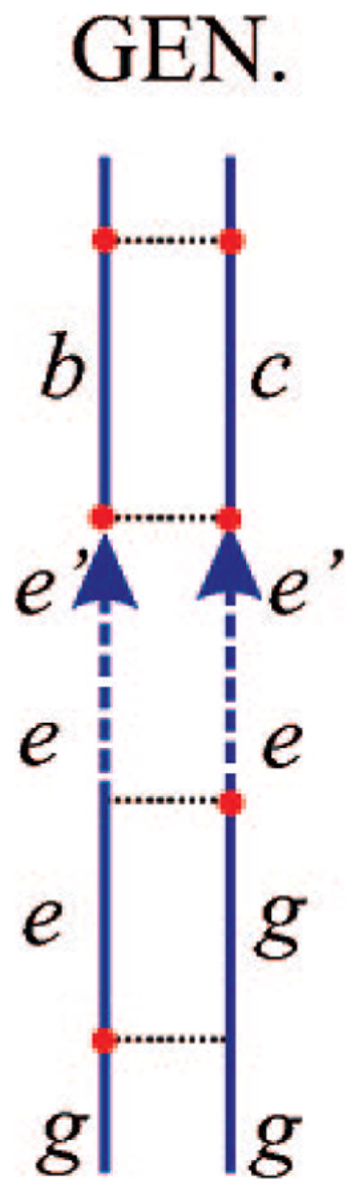
Generalized diagram with population relaxation showing three density matrix propagation intervals. By a proper choice of the b and c states, this diagram can represent the density matrix evolution of all diagrams in Figure 7.

$${\mathbb{F}}_{cb{e}^{\prime }e}^{(I)}(t_3,t_2,t_1)={\text{e}}^{i{\omega }_{cb}{t}_3-i{\epsilon }_e{t}_1}\times \langle {\text{e}}^{+i{\widehat{H}}_{e^{\prime }}{t}_2+i{\widehat{H}}_c{t}_3-i{\widehat{H}}_b{t}_3-i{\widehat{H}}_{e^{\prime }}{t}_2-i{\widehat{H}}_e{t}_1}\rangle .$$ (414)

Here, we assumed that the bath dynamics for different exciton states is correlated; a simpler case is given in ref 24. is evaluated by the cumulant expansion, and we get

$${\mathbb{F}}_{cb{e}^{\prime }e}^{(I)}(t_3,t_2,t_1)=exp[i{\omega }_{cb}{t}_3-i{\epsilon }_e{t}_1-({\tau }_c^{-1}+{\tau }_b^{-1})t_3-{\tau }_e^{-1}{t}_1+{\overline{\phi }}_{cb{e}^{\prime }e}(t_3,t_2,t_1)],$$ (415)

where

$${\overline{\phi }}_{cb{e}^{\prime }e}(t_3,t_2,t_1)=-g_{ee}(t_1)-g_{bb}(t_3)-g_{cc}^{\ast }(t_3)-g_{be}(t_1+t_2+t_3)+g_{be}(t_1+t_2)+g_{be}(t_2+t_3)+g_{ce}(t_1+t_2+t_3)-g_{ce}(t_1+t_2)-g_{be}(t_2+t_3)+g_{cb}(t_3)+g_{bc}^{\ast }(t_3)+g_{ce}(t_2)-g_{be}(t_2)+2iIm[g_{c{e}^{\prime }}(t_2+t_3)-g_{c{e}^{\prime }}(t_2)-g_{c{e}^{\prime }}(t_3)+g_{b{e}^{\prime }}(t_2)-g_{b{e}^{\prime }}(t_2+t_3)+g_{b{e}^{\prime }}(t_3)].$$ (416)

Here, Im denotes the imaginary part. This expression contains line-shape functions that represent correlations during the time intervals t₁ and t₃.

The contribution of population-conserving terms to the response function now coincides with the coherent description. The contribution of the population-transfer diagram can be calculated using the cumulant expansion of

$$R_P^{(3)}(t_3,t_2,t_1)=\sum _p\sum _{{\nu }_p{e}^{\prime }e}{(-1)}^p{\mathbb{G}}_{e^{\prime }{e}^{\prime },ee}^{(N)}(t_2){\langle {\mathbb{W}}_{bc}^{pp}(t_3){\mathbb{D}}_{eg}^{rl}(t_1)\rangle }^p,$$ (417)

where p denotes the summation over ia, iiia, iva, and via pathways: for ia, we have (–1)^p ≡ 1, ν_p ≡ g, c ≡ e′, b ≡ g, ≡ , 〈... 〉 ^p 〈 ... 〉 *; for iiia, we have (–1)^p ≡ –1, ν_p ≡ f, c ≡ f, b = e′, ≡ , 〈... 〉^p ≡ 〈... 〉*; for iva, we have (–1)^p ≡ 1, ν_p ≡ g, c ≡ g, b ≡ e′, ≡ , 〈 ... 〉^p ≡ 〈 ... 〉; for via, we have (–1)^p ≡ –1, ν_p ≡ f, c ≡ e′, b ≡ f, ≡ , 〈... 〉^p ≡ 〈... 〉. We next use μ_ab = μ_ba and the correlation function of eq 414. These yield in the following expression

$$R_P^{(3)}(t_3,t_2,t_1)={(i{\hslash }^{-1})}^3\sum _p\sum _{{\nu }_p{e}^{\prime }e}{(-1)}^p{\mathit{\mu }}_{cb}{\mathit{\mu }}_{{\nu }_p{e}^{\prime }}{\mathit{\mu }}_{eg}{\mathit{\mu }}_{eg}\times {\mathbb{G}}_{e^{\prime }{e}^{\prime },ee}^{(N)}(t_2){[{\mathbb{F}}_{cb{e}^{\prime }e}^{(I)}(t_3,t_2,t_1)]}^p.$$ (418)

The dynamics of solely comes from the doorway and window functions. The phase functions in eq 179 are obtained from eq 418 by sorting out all Liouville space pathways.

28. Appendix L: Orientationally Averaged Molecular Properties

Here, we present expressions for third-order signals in isotropic ensembles of molecules. As shown in eq 251, the response function has several linearly independent configurations that differ by the polarization ν and wavevector k orientations in the laboratory coordinate frame. The complete expressions for this pulse-polarization configuration for the linear response are

$$\langle {\mathit{J}}_2^{{\nu }_2}{\mathit{J}}_1^{{\nu }_1}\rangle ={\omega }^2\{\langle {\mathit{\mu }}_2^{{\nu }_2}{\mathit{\mu }}_1^{{\nu }_1}\rangle +\frac{2\pi i}{\lambda }[\langle {\mathit{q}}_2^{{\kappa }_2,{\nu }_2}{\mathit{\mu }}_1^{{\nu }_1}\rangle -\langle {\mathit{\mu }}_2^{{\nu }_2}{\mathit{q}}_1^{{\kappa }_1,{\nu }_1}\rangle ]+\frac{i}{c}\sum _{\alpha }[{\epsilon }_{{\nu }_2{\kappa }_2\alpha }\langle {\mathit{m}}_2^{″\alpha }{\mathit{\mu }}_1^{{\nu }_1}\rangle -{\epsilon }_{{\nu }_1{\kappa }_1\alpha }\langle {\mathit{\mu }}_2^{{\nu }_2}{\mathit{m}}_1^{″\alpha }\rangle ]\}.$$ (419)

For third-order techniques, we set k_I ≡ (u, v, w) = (–1, 1, 1), for k_II ≡ (u, v, w) = (1, –1, 1), and for k_III ≡ (u, v, w) = (1, 1, –1). We then get

$$\langle {\mathit{J}}_4^{{\nu }_4}{\mathit{J}}_3^{{\nu }_3}(w){\mathit{J}}_2^{{\nu }_2}(v){\mathit{J}}_1^{{\nu }_1}(u)\rangle ={\omega }^4\{\langle {\mathit{\mu }}_4^{{\nu }_4}{\mathit{\mu }}_3^{{\nu }_3}{\mathit{\mu }}_2^{{\nu }_2}{\mathit{\mu }}_1^{{\nu }_1}\rangle +\frac{2\pi i}{\lambda }[\langle {\mathit{q}}_4^{{\kappa }_4,{\nu }_4}{\mathit{\mu }}_3^{{\nu }_3}{\mathit{\mu }}_2^{{\nu }_2}{\mathit{\mu }}_1^{{\nu }_1}\rangle -w\langle {\mathit{\mu }}_4^{{\nu }_4}{\mathit{q}}_3^{{\kappa }_3,{\nu }_3}{\mathit{\mu }}_2^{{\nu }_2}{\mathit{\mu }}_1^{{\nu }_1}\rangle -v\langle {\mathit{\mu }}_4^{{\nu }_4}{\mathit{\mu }}_3^{{\nu }_3}{\mathit{q}}_2^{{\kappa }_2,{\nu }_2}{\mathit{\mu }}_1^{{\nu }_1}\rangle -u\langle {\mathit{\mu }}_4^{{\nu }_4}{\mathit{\mu }}_3^{{\nu }_3}{\mathit{\mu }}_2^{{\nu }_2}{\mathit{q}}_1^{{\kappa }_1,{\nu }_1}\rangle ]+\frac{i}{c}\sum _{\alpha }[{\epsilon }_{{\nu }_4{\kappa }_4\alpha }\langle {\mathit{m}}_4^{″\alpha }{\mathit{\mu }}_3^{{\nu }_3}{\mathit{\mu }}_2^{{\nu }_2}{\mathit{\mu }}_1^{{\nu }_1}\rangle -w{\epsilon }_{{\nu }_3{\kappa }_3\alpha }\langle {\mathit{\mu }}_4^{{\nu }_4}{\mathit{m}}_3^{″\alpha }{\mathit{\mu }}_2^{{\nu }_2}{\mathit{\mu }}_1^{{\nu }_1}\rangle -u{\epsilon }_{{\nu }_2{\kappa }_2\alpha }\langle {\mathit{\mu }}_4^{{\nu }_4}{\mathit{\mu }}_3^{{\nu }_3}{\mathit{m}}_2^{″\alpha }{\mathit{\mu }}_1^{{\nu }_1}\rangle -\upsilon {\epsilon }_{{\nu }_1{\kappa }_1\alpha }\langle {\mathit{\mu }}_4^{{\nu }_4}{\mathit{\mu }}_3^{{\nu }_3}{\mathit{\mu }}_2^{{\nu }_2}{\mathit{m}}_1^{″\alpha }\rangle ]\},$$ (420)

where ε_γαβ is the antisymmetric Levi–Civita tensor. These can be obtained from orientational averaging of tensor products of arbitrary sets of vectors d_i and second-rank tensors t_i

$$\langle {\mathit{d}}_2^{{\nu }_2}{\mathit{d}}_1^{{\nu }_1}\rangle =\frac{1}{3}({\mathit{\nu }}_2·{\mathit{\nu }}_1)({\mathit{d}}_2·{\mathit{d}}_1),$$ (421)

$$\langle {\mathit{t}}_2^{\kappa {\nu }_2}{\mathit{d}}_1^{{\nu }_1}\rangle =\frac{1}{6}(\kappa ·({\mathit{\nu }}_2\times {\mathit{\nu }}_1)({\mathit{d}}_1\odot {\mathit{t}}_2),$$ (422)

$$\langle {\mathit{d}}_2^{{\nu }_2}{\mathit{t}}_1^{\kappa {\nu }_1}\rangle =-\frac{1}{6}(\kappa ·({\mathit{\nu }}_2\times {\mathit{\nu }}_1)({\mathit{d}}_2\odot {\mathit{t}}_1),$$ (423)

$$\langle {\mathit{d}}_4^{{\nu }_4}{\mathit{d}}_3^{{\nu }_3}{\mathit{d}}_2^{{\nu }_2}{\mathit{d}}_1^{{\nu }_1}\rangle ={\mathit{F}}_{\{\nu \}}^{(4)\text{T}}{\mathit{M}}^{(4)}{\mathit{V}}^{(4)},$$ (424)

$$\langle {\mathit{t}}_4^{{\nu }^{\prime }{\nu }_4}{\mathit{d}}_3^{{\nu }_3}{\mathit{d}}_2^{{\nu }_2}{\mathit{d}}_1^{{\nu }_1}\rangle ={\mathit{F}}_{\{\nu \}}^{(5)\text{T}}{\mathit{M}}^{(5)}{\mathit{V}}_4^{(5)},$$ (425)

$$\langle {\mathit{d}}_4^{{\nu }_4}{\mathit{t}}_3^{{\nu }^{\prime }{\nu }_3}{\mathit{d}}_2^{{\nu }_2}{\mathit{d}}_1^{{\nu }_1}\rangle ={\mathit{F}}_{\{\nu \}}^{(5)\text{T}}{\mathit{M}}^{(5)}{\mathit{V}}_3^{(5)},$$ (426)

$$\langle {\mathit{d}}_4^{{\nu }_4}{\mathit{d}}_3^{{\nu }_3}{\mathit{t}}_2^{{\nu }^{\prime }{\nu }_2}{\mathit{d}}_1^{{\nu }_1}\rangle ={\mathit{F}}_{\{\nu \}}^{(5)\text{T}}{\mathit{M}}^{(5)}{\mathit{V}}_2^{(5)},$$ (427)

$$\langle {\mathit{d}}_4^{{\nu }_4}{\mathit{d}}_3^{{\nu }_3}{\mathit{d}}_2^{{\nu }_2}{\mathit{t}}_1^{{\nu }^{\prime }{\nu }_1}\rangle ={\mathit{F}}_{\{\nu \}}^{(5)\text{T}}{\mathit{M}}^{(5)}{\mathit{V}}_1^{(5)},$$ (428)

${\mathit{F}}_{\{\nu \}}^{(N)}$ are column vectors that depend on the laboratory-frame unit vectors ν:

$${\mathit{F}}_{\{\nu \}}^{(4)}=\left(\begin{array}{c}({\mathit{\nu }}_4·{\mathit{\nu }}_3)({\mathit{\nu }}_2·{\mathit{\nu }}_1)\\ ({\mathit{\nu }}_4·{\mathit{\nu }}_2)({\mathit{\nu }}_3·{\mathit{\nu }}_1)\\ ({\mathit{\nu }}_4·{\mathit{\nu }}_1)({\mathit{\nu }}_3·{\mathit{\nu }}_2)\end{array}\right),$$ (429)

$${\mathit{F}}_{\{\nu \}}^{(5)}=\left(\begin{array}{c}{\mathit{\nu }}_4·({\mathit{\nu }}_3\times {\mathit{\nu }}_2)({\mathit{\nu }}_1·{\mathit{\nu }}^{\prime })\\ {\mathit{\nu }}_4·({\mathit{\nu }}_3\times {\mathit{\nu }}_1)({\mathit{\nu }}_2·{\mathit{\nu }}^{\prime })\\ {\mathit{\nu }}_4·({\mathit{\nu }}_3\times {\mathit{\nu }}^{\prime })({\mathit{\nu }}_2·{\mathit{\nu }}_1)\\ {\mathit{\nu }}_4·({\mathit{\nu }}_2\times {\mathit{\nu }}_1)({\mathit{\nu }}_3·{\mathit{\nu }}^{\prime })\\ {\mathit{\nu }}_4·({\mathit{\nu }}_2\times {\mathit{\nu }}^{\prime })({\mathit{\nu }}_3·{\mathit{\nu }}_1)\\ {\mathit{\nu }}_4·({\mathit{\nu }}_1\times {\mathit{\nu }}^{\prime })({\mathit{\nu }}_3·{\mathit{\nu }}_2)\end{array}\right),$$ (430)

The matrices M are system-independent:

$$M^{(4)}=\frac{1}{30}\left(\begin{array}{rrr}\hfill 4& \hfill -1& \hfill -1\\ \hfill -1& \hfill 4& \hfill -1\\ \hfill -1& \hfill -1& \hfill 4\end{array}\right),$$ (431)

$$M^{(5)}=\frac{1}{30}\left(\begin{array}{rrrrrr}\hfill 3& \hfill -1& \hfill -1& \hfill 1& \hfill 1& \hfill 0\\ \hfill -1& \hfill 3& \hfill -1& \hfill -1& \hfill 0& \hfill 1\\ \hfill -1& \hfill -1& \hfill 3& \hfill 0& \hfill -1& \hfill -1\\ \hfill 1& \hfill -1& \hfill 0& \hfill 3& \hfill -1& \hfill 1\\ \hfill 1& \hfill 0& \hfill -1& \hfill -1& \hfill 3& \hfill -1\\ \hfill 0& \hfill 1& \hfill -1& \hfill 1& \hfill -1& \hfill 3\end{array}\right).$$ (432)

Finally, V are column vectors that depend on the system properties:

$$V^{(4)}=\left(\begin{array}{c}({\mathit{d}}_4·{\mathit{d}}_3)({\mathit{d}}_2·{\mathit{d}}_1)\\ ({\mathit{d}}_4·{\mathit{d}}_2)({\mathit{d}}_3·{\mathit{d}}_1)\\ ({\mathit{d}}_4·{\mathit{d}}_1)({\mathit{d}}_3·{\mathit{d}}_2)\end{array}\right),$$ (433)

$$V_4^{(5)}=\left(\begin{array}{c}{\mathit{d}}_1·{\mathit{t}}_4·({\mathit{d}}_3\times {\mathit{d}}_2)\\ {\mathit{d}}_2·{\mathit{t}}_4·({\mathit{d}}_3\times {\mathit{d}}_1)\\ ({\mathit{d}}_3\odot {\mathit{t}}_4)({\mathit{d}}_2·{\mathit{d}}_1)\\ {\mathit{d}}_3·{\mathit{t}}_4·({\mathit{d}}_2\times {\mathit{d}}_1)\\ ({\mathit{d}}_2\odot {\mathit{t}}_4)({\mathit{d}}_3·{\mathit{d}}_1)\\ ({\mathit{d}}_1\odot {\mathit{t}}_4)({\mathit{d}}_3·{\mathit{d}}_2)\end{array}\right),$$ (434)

$$V_3^{(5)}=\left(\begin{array}{c}{\mathit{d}}_1·{\mathit{t}}_3·({\mathit{d}}_2\times {\mathit{d}}_4)\\ {\mathit{d}}_2·{\mathit{t}}_3·({\mathit{d}}_1\times {\mathit{d}}_4)\\ -({\mathit{d}}_4\odot {\mathit{t}}_3)({\mathit{d}}_2·{\mathit{d}}_1)\\ {\overline{\mathit{t}}}_3({\mathit{d}}_4·({\mathit{d}}_2\times {\mathit{d}}_1))\\ ({\mathit{d}}_4\times {\mathit{d}}_2)·{\mathit{t}}_3·{\mathit{d}}_1\\ ({\mathit{d}}_4\times {\mathit{d}}_1)·{\mathit{t}}_3·{\mathit{d}}_2\end{array}\right),$$ (435)

$$V_2^{(5)}=\left(\begin{array}{c}{\mathit{d}}_1·{\mathit{t}}_2·({\mathit{d}}_4\times {\mathit{d}}_3)\\ {\overline{\mathit{t}}}_2({\mathit{d}}_4·({\mathit{d}}_3\times {\mathit{d}}_1))\\ ({\mathit{d}}_4\times {\mathit{d}}_3)·{\mathit{t}}_2·{\mathit{d}}_1\\ {\mathit{d}}_3·{\mathit{t}}_2·({\mathit{d}}_1\times {\mathit{d}}_4)\\ -({\mathit{d}}_4\odot {\mathit{t}}_2)({\mathit{d}}_3·{\mathit{d}}_1)\\ ({\mathit{d}}_4\times {\mathit{d}}_1)·{\mathit{t}}_2·{\mathit{d}}_3\end{array}\right),$$ (436)

$$V_1^{(5)}=\left(\begin{array}{c}{\mathit{t}}_1{\mathit{d}}_4·({\mathit{d}}_3\times {\mathit{d}}_2)\\ {\mathit{d}}_2·{\mathit{t}}_1·({\mathit{d}}_4\times {\mathit{d}}_3)\\ ({\mathit{d}}_4\times {\mathit{d}}_3)·{\mathit{t}}_1·{\mathit{d}}_2\\ {\mathit{d}}_3·{\mathit{t}}_1·({\mathit{d}}_4\times {\mathit{d}}_2)\\ ({\mathit{d}}_4\times {\mathit{d}}_2)·{\mathit{t}}_1·{\mathit{d}}_3\\ -({\mathit{d}}_4\odot {\mathit{t}}_1)({\mathit{d}}_3·{\mathit{d}}_2)\end{array}\right),$$ (437)

where d⊙t ≡ Σ_{α3α 2α 1}ε_{α 3α 2α 1}d^{α ₃}t^{α ₂α ₁}, (t•d)^α ≡ Σ_α′t^αα′d^α′, (d•t)^α ≡ Σ_α′ d^α′t^{α ′α}, and t ≡ Σ_αt^αα; consequently, ${\mathit{d}}_1·\mathit{t}·{\mathit{d}}_2\equiv {\sum }_{{\alpha }_1{\alpha }_2}{\mathit{d}}_1^{{\alpha }_1}{\mathit{t}}^{{\alpha }_1{\alpha }_2}{\mathit{d}}_2^{{\alpha }_2}$. By comparing with eqs 419 and 420 and replacing the vectors d with μ and m and the tensors t with quadrupoles q, we can calculate the orientationally averaged currents.

For the linear response in the exciton basis, we have ${\mathit{J}}_2={\mathit{J}}_1^{\ast }$ and the signal must propagate in the same direction of the incoming field. We can thus set κ = z. Orientational averaging for exciton e gives

$$\langle {\mathit{J}}_e^{{\nu }_2}{\mathit{J}}_e^{{\nu }_1\ast }\rangle ={\omega }^2\frac{1}{3}\{{\delta }_{{\nu }_2{\nu }_1}{\mid {\mathit{\mu }}_e\mid }^2-i(\mathit{k}·({\mathit{\nu }}_2\times {\mathit{\nu }}_1))\times [{\mathit{\mu }}_e\odot {\mathit{q}}_e-2m_e^{″}·{\mathit{\mu }}_e]\}.$$ (438)

The orientational factors given by eqs 424–437 relate the signals to molecular geometry. The CI terms can be identified by examining the products of transition dipoles. The electric transition dipole μ_ξ and coordinate r_m are parity-odd, while the magnetic transition dipole m_ξ and tensors q_ξ are even. By performing the parity operation on the response functions and inspecting the parity symmetry, we can connect the susceptibility with the chirality. All zero-order in wavevector contributions to odd (linear and cubic) response must be NC, since they involve either two or four electric transition dipoles. The corresponding first-order contributions in wavevectors are CI.