Systematic Removal of Outliers to Reduce Heterogeneity in Case-Control Association Studies

Abstract

Background/Aims

In human case-control association studies, population heterogeneity is often present and can lead to increased false-positive results. Various methods have been proposed and are in current use to remedy this situation.

Methods

We assume that heterogeneity is due to a relatively small number of individuals whose allele frequencies differ from those of the remainder of the sample. For this situation, we propose a new method of handling heterogeneity by removing outliers in a controlled manner. In a coordinate system of the c largest principal components in multidimensional scaling (MDS), we systematically remove one after another of the most extreme outlying individuals and each time recompute the largest association test statistic. The smallest p value obtained within M removals serves as our test statistic whose significance level is assessed in randomization samples.

Results

In power simulations of our method and three methods in current use, averaged over several different scenarios, the best method turned out to be logistic regression analysis (based on all individuals) with MDS components as covariates.

Conclusion

Our proposed method ranked closely behind logistic regression analysis with MDS components but ahead of other commonly used approaches. In analyses of real datasets our method performed best.

Background

Population admixture (cryptic heterogeneity) represents a potentially serious problem in case-control association studies [1]. Allele frequencies tend to differ between countries and even between different regions in a single country [2,3]. Disregarding such differences tends to inflate the χ² association statistic [4], which ‘sees’ heterogeneity as a deviation from the null hypothesis of homogeneity. One of the first methods to deal with the deleterious effects of heterogeneity is genomic control (GC) [4], which assesses the extent of inflation of χ² in terms of the GC factor, λ, and then divides each χ² by λ. Additional methods have since been introduced, notably principal components analysis [5] and logistic regression with components of multidimensional scaling (MDS) as covariates [6]. Here, we propose a novel approach based on deleting individuals that appear as outliers. This approach specifically addresses the situation of a relatively small number of individuals that do not belong to the main portion of the study sample.

Outlier Removal Method

It is intuitive that one way to deal with heterogeneity is to remove individuals not belonging to a sample. Such an approach might be seen as more appropriate than ‘punishing’ all individuals by rolling back all test statistics as it is done in the GC method. However, removing outliers has to be carried out in a statistically satisfactory manner. To decide how many and which individuals to remove, we proceed as follows: based on the commonly used identity by state (IBS) metric, similarity between two individuals is defined as the IBS between two individuals, averaged over all SNPs. In the coordinate system of the c largest MDS components (here we use c = 4 throughout), each individual is at some distance from the center. That individual with the largest distance from the center is considered a potential outlier.

Initially, the Pearson χ² is computed in a 2 × 2 contingency table for each SNP, where the two rows correspond to cases and controls, and the two columns represent the SNP alleles. After retaining the p value, p₀, for the largest χ² over all the SNPs, the first potential outlier is removed and another largest χ² is computed (at whatever SNP in the genome it occurs) leading to p₁, and so on. We proceed until a predefined maximum number, M, of individuals has been removed. The sequence of p values (p₀, p₁, …, p_M) initially either decreases (p₀ > p₁) or increases (p₀ < p₁). In the first case, assume that the smallest p value, p_min, among the M + 1 values occurs at step k, that is, after k outliers have been removed. We then take T = p_min as our overall test statistic. In the latter case, we search for the first (local) minimum p value, T, or, if none occurs, we retain T = p_M, with T again being our test statistic. In each of a sufficiently large set of randomization samples (labels case and control are randomly permuted), the whole approach is repeated, and we obtain the significance level associated with T as the proportion of randomization samples with T values at least as small as the observed T. Note that there may be a different SNP with largest χ² in different steps of outlier removal.

The technique of finding the smallest p value among several model assumptions and obtaining the (genome-wide) significance level associated with this smallest p value is not new. We previously applied this principle in comparing disease association of sets of SNPs, where each set contains different numbers of SNPs. This has led to our Set Association method [7], which is more powerful than SNP by SNP analysis [8,9] and has successfully been applied in various studies [10,11,12].

By design, our approach always removes at least one individual. In this sense, it furnishes trimmed results. Trimming is well known in classical statistics as a procedure for eliminating outliers [13,14]. In particular, such methods have been developed for small numbers of outlying observations [15]. Here we apply this principle to case-control association studies.

Power Simulations

For a simple power comparison, we assume a total of 1,000 independent SNPs, with the last SNP conferring disease susceptibility. We further assume a total sample size of 200 individuals, of which 10 are outliers. The 190 non-outliers are equally divided into cases and controls while we consider 3 scenarios for the 10 outliers: (1) 5 cases and 5 controls, (2) 2 cases and 8 controls, and (3) no cases and 10 controls, where the latter scenario represents the (perhaps common) situation that controls tend to be chosen from a different population segment than that furnishing cases. For the 999 non-disease SNPs with alleles A and B, allele frequencies P(A) are randomly picked between 0.10 and 0.50 for non-outliers, and between 0.10 and 0.90 for outliers (for details, see online suppl. material; for all online suppl. material, see www.karger.com/doi/10.1159/000320422).

The disease (functional) SNP has alleles D and d, with the former conferring disease susceptibility. Its allele frequency, P(D), is set to 0.30 in non-outliers and is chosen randomly from 0.10 through 0.90 in outliers. Genotype frequencies are given according to the Hardy Weinberg equilibrium. We consider dominant and recessive inheritance, with h denoting the penetrance for non-susceptibility genotypes, while the penetrance for disease conferring genotypes is given by rh. Disease prevalence is taken to be 1%. Power to detect the disease SNP is computed as a function of the penetrance ratio, r = rh/h, where r = 1 represents the null hypothesis of no genetic effect. The maximum number of outliers to be removed is set at M = 20 (10% of the sample size of 200).

We compare the following 4 test procedures, where each is applied to the disease SNP. The remaining SNPs are independent of the disease SNP.

• (1)Pearson-GC: This 1 d.f. Pearson χ² test with GC correction, that is, all χ² are divided by the GC parameter, λ, where λ = observed median χ² for all SNPs divided by the median of the χ² distribution with 1 d.f. (0.456).
• (2)Logistic: Logistic regression analysis for each SNP in turn, additive allele test (1 d.f.). This test has no provision for addressing the heterogeneity problem.
• (3)Logistic-MDS: Logistic regression analysis (1 d.f.) with the largest 4 MDS components as covariates. The latter are determined on the basis of all SNPs.
• (4)Outliers: Our approach for removing individuals that extremely deviate from the center in an MDS coordinate space.

At r = 1, for each of the 4 methods, 5,000 datasets are generated under dominant and recessive inheritance, and critical thresholds for the test statistics are chosen such that the resulting significance level (proportion of significant results) is exactly equal to 0.05. Resulting thresholds are then used to estimate power at penetrance ratios r > 1.

Results

Power of the different analysis methods was somewhat dependent on model assumptions, but the Logistic-MDS method overall did best, followed by our Outliers method. Table 1 shows results for dominant inheritance and outliers consisting of 2 cases and 8 controls (all results of power simulations are given in online suppl. table S1); these results are fairly typical of the overall picture. Figure 1 shows power figures in graphical form.

Table 1.

Power of 4 association analysis methods as a function of the penetrance ratio, r, for a dominant disease model

	Pearson-CG	Logistic	Logistic-MDS	Outliers
r = 1.0	0.050	0.050	0.050	0.050
r = 1.5	0.132	0.149	0.232	0.176
r = 2.0	0.392	0.427	0.557	0.463
r = 2.5	0.615	0.663	0.777	0.685
r = 3.0	0.761	0.804	0.894	0.817
r = 3.5	0.853	0.887	0.941	0.891
r = 4.0	0.906	0.934	0.970	0.938
Average power	0.513	0.512	0.594	0.572
Rank	3	4	1	2

The number of outliers is 10 (2 cases, 8 controls), and the number of non-outliers is 190. The last two rows show average power over 36 model conditions (shown in online suppl. table S1) and resulting ranking.

Fig. 1.

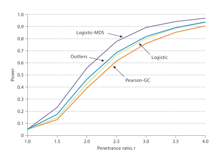
Power of 4 analysis methods as a function of the penetrance ratio, r (based on results in table 1).

We combined results for each value of r and 6 model assumptions (dominant/recessive, 3 splits of cases versus controls in outliers) and computed average power over these 36 conditions (online suppl. table S1). As the last row of table 1 shows, this ranking makes the Logistic-MDS method the winner, closely followed by our Outliers method. This power simulation is rather simple and is mainly designed to demonstrate that our Outliers method is competitive. In particular, only one disease SNP was assumed and any significant result is a true positive. Additional power simulations are provided in the online supplementary material, for example, for a trait influenced by two susceptibility loci and for different population structures. The Pearson-GC method presumably suffers from the potentially severe protection from false-positive results. In fact, computing p values from χ² tables for the Pearson-GC method leads to type I errors much smaller than 0.05 (details not shown) but, as mentioned, in our simulations the type I error was constant for all methods.

Analyzing a Published Dataset

To demonstrate our Outliers method, we applied it and the 3 other approaches discussed here to a published dataset on Parkinson disease with approximately 540 case and control individuals and approximately 408,000 SNPs genome wide [16]. To make results comparable and allow for genome-wide correction for multiple testing, p values were estimated in permutation samples. In this analysis, we applied the standard Pearson χ² test without GC correction.

As table 2 shows, the Outliers method furnished the smallest p value of 0.076, which is not formally significant, although nearly so. The smallest nominal p value in the Outliers method was obtained after 3 individuals had been removed as outliers (fig. 2). The significance level associated with this smallest p value is estimated to be 0.076. Without removing outliers, the p value of the largest test statistic (χ²) is equal to 0.120. Thus, the Outliers method resulted in a considerable improvement, although it did not furnish a significant result. If, for argument's sake, we transform p values into χ² with 2 d.f. [17], we find χ² of c₁ = 5.15 for p = 0.076, and c₂ = 4.24 for p = 0.120. As χ² is proportional to sample size, the ratio, c₁/c₂ = 1.22, reflects a virtual gain of 22% in sample size obtained by our method. Of course, this argument is artificial since we do not know whether these p values reflect true or false positives.

Table 2.

Analysis results for a published dataset of Parkinson Disease

Logistic-MDS					Logistic
ch	SNP	pos	Pnom	Pperm	ch	SNP	pos	Pnom	Pperm
4	rs6826751	68262621	1.73E-06	0.232	4	rs6826751	68262621	2.46E-06	0.258
4	rs2242330	68276015	5.64E-06	0.590	4	rs2242330	68276015	6.05E-06	0.569
4	rs3775866	68272946	1.03E-05	0.827	4	rs3775866	68272946	1.11E-05	0.831
4	rs355477	68225291	1.83E-05	0.970	16	rs4888984	78066835	1.30E-05	0.877
4	rs355461	68209490	1.87E-05	0.972	4	rs355477	68225291	1.63E-05	0.935
4	rs355506	68214848	1.87E-05	0.972	10	rsl480597	44481115	1.67E-05	0.940
10	rsl480597	44481115	1.92E-05	0.973	4	rs355461	68209490	1.73E-05	0.948
5	rsl0053056	96069176	1.92E-05	0.973	4	rs355506	68214848	1.73E-05	0.948
1	rsl887279	180641817	1.94E-05	0.974	1	rsl887279	180641817	1.83E-05	0.954
16	rs4888984	78066835	1.95E-05	0.974	4	rs355464	68207890	1.91E-05	0.959

Outliers (3 removed)					Pearson-GC
ch	SNP	pos	Pnom	Pperm	ch	SNP	pos	Pnom	Pperm
4	rs6826751	68262621	2.35E-07	0.076	4	rs6826751	68262621	5.51E-07	0.120
4	rs2242330	68276015	1.74E-06	0.477	4	rs2242330	68276015	3.33E-06	0.602
4	rs355464	68207890	4.00E-06	0.775	4	rs355464	68207890	7.28E-06	0.868
4	rs355461	68209490	4.04E-06	0.778	4	rs355461	68209490	7.33E-06	0.871
4	rs355506	68214848	4.04E-06	0.778	4	rs355506	68214848	7.33E-06	0.871
4	rs355477	68225291	4.11E-06	0.780	4	rs355477	68225291	7.47E-06	0.879
4	rs3775866	68272946	4.52E-06	0.815	4	rs3775866	68272946	7.88E-06	0.890
4	rsll946612	68164737	4.56E-06	0.817	4	rsll946612	68164737	8.27E-06	0.901
4	rsl497430	68186580	4.56E-06	0.817	4	rsl497430	68186580	8.27E-06	0.901
4	rs9312181	68165345	5.40E-06	0.871	1	rsl887279	180641817	9.27E-06	0.922

ch = Chromosome; pos = position; p_nom = nominal p value; Pp_erm = P value from permutation samples, corrected for multiple testing, 1,000 permutations.

Fig. 2.

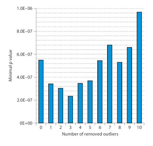
For Parkinson disease dataset, minimum p values obtained with given numbers of outliers removed.

Discussion

So-called ‘obvious’ outliers are often removed in an ad-hoc manner, and there may not be good statistical justifications for doing so. In particular, if outliers are removed by trial and error, that is, if they are removed only when this leads to a reduction in p value, then such a procedure clearly tends to increase the false-positive rate of results. Here, we developed a statistically rigorous procedure for removing outliers while maintaining correct type I error.

We carried out additional power simulations under various conditions and also analyzed one more real dataset. All these results may be found in the online supplementary material. These simulations confirm our conclusions based on results shown in table 1; they also show that the Outliers method often does best with recessive modes of inheritance. In addition, at least in the two real datasets analyzed here, for the best SNPs, the Outliers method yields the smallest p values.

As is well known, an alternative to removing outliers is to allow for them in the analysis, which may be done by including principal components as covariates in logistic regression analysis [5]. The two approaches may do equally well in practice, although our power calculations have given the logistic regression approach (with MDS components) a slight advantage.

Supplementary Material

Supplemental Data

References

- 1.Pritchard JK, Stephens M, Rosenberg NA, Donnelly P. Association mapping in structured populations. Am J Hum Genet. 2000;67:170–181. doi: 10.1086/302959. [DOI] [PMC free article] [PubMed] [Google Scholar]
- 2.Xu S, Yin X, Li S, Jin W, Lou H, Yang L, Gong X, Wang H, Shen Y, Pan X, He Y, Yang Y, Wang Y, Fu W, An Y, Wang J, Tan J, Qian J, Chen X, Zhang X, Sun Y, Zhang X, Wu B, Jin L. Genomic dissection of population substructure of Han Chinese and its implication in association studies. Am J Hum Genet. 2009;85:762–774. doi: 10.1016/j.ajhg.2009.10.015. [DOI] [PMC free article] [PubMed] [Google Scholar]
- 3.Chen J, Zheng H, Bei JX, Sun L, Jia WH, Li T, Zhang F, Seielstad M, Zeng YX, Zhang X, Liu J. Genetic structure of the Han Chinese population revealed by genome-wide SNP variation. Am J Hum Genet. 2009;85:775–785. doi: 10.1016/j.ajhg.2009.10.016. [DOI] [PMC free article] [PubMed] [Google Scholar]
- 4.Devlin B, Roeder K. Genomic control for association studies. Biometrics. 1999;55:997–1004. doi: 10.1111/j.0006-341x.1999.00997.x. [DOI] [PubMed] [Google Scholar]
- 5.Price AL, Patterson NJ, Plenge RM, Weinblatt ME, Shadick NA, Reich D. Principal components analysis corrects for stratification in genome-wide association studies. Nat Genet. 2006;38:904–909. doi: 10.1038/ng1847. [DOI] [PubMed] [Google Scholar]
- 6.Purcell S, Neale B, Todd-Brown K, Thomas L, Ferreira MA, Bender D, Maller J, Sklar P, de Bakker PI, Daly MJ, Sham PC. PLINK: a tool set for whole-genome association and population-based linkage analyses. Am J Hum Genet. 2007;81:559–575. doi: 10.1086/519795. [DOI] [PMC free article] [PubMed] [Google Scholar]
- 7.Hoh J, Wille A, Ott J. Trimming, weighting, and grouping SNPs in human case-control association studies. Genome Res. 2001;11:2115–2119. doi: 10.1101/gr.204001. [DOI] [PMC free article] [PubMed] [Google Scholar]
- 8.Hao K, Xu X, Laird N, Wang X, Xu X. Power estimation of multiple SNP association test of case-control study and application. Genet Epidemiol. 2004;26:22–30. doi: 10.1002/gepi.10293. [DOI] [PubMed] [Google Scholar]
- 9.Heidema AG, Feskens EJ, Doevendans PA, Ruven HJ, van Houwelingen HC, Mariman EC, Boer JM. Analysis of multiple SNPs in genetic association studies: comparison of three multi-locus methods to prioritize and select SNPs. Genet Epidemiol. 2007;31:910–921. doi: 10.1002/gepi.20251. [DOI] [PubMed] [Google Scholar]
- 10.Papassotiropoulos A, Wollmer MA, Tsolaki M, Brunner F, Molyva D, Lutjohann D, Nitsch RM, Hock C. A cluster of cholesterol-related genes confers susceptibility for Alzheimer's disease. J Clin Psychiatry. 2005;66:940–947. [PubMed] [Google Scholar]
- 11.Kankova K, Stejskalova A, Pacal L, Tschoplova S, Hertlova M, Krusova D, Izakovicova-Holla L, Beranek M, Vasku A, Barral S, Ott J. Genetic risk factors for diabetic nephropathy on chromosomes 6p and 7q identified by the set-association approach. Diabetologia. 2007;50:990–999. doi: 10.1007/s00125-007-0606-3. [DOI] [PubMed] [Google Scholar]
- 12.Cavalleri GL, Weale ME, Shianna KV, Singh R, Lynch JM, Grinton B, Szoeke C, Murphy K, Kinirons P, O'Rourke D, Ge D, Depondt C, Claeys KG, Pandolfo M, Gumbs C, Walley N, McNamara J, Mulley JC, Linney KN, Sheffield LJ, Radtke RA, Tate SK, Chissoe SL, Gibson RA, Hosford D, Stanton A, Graves TD, Hanna MG, Eriksson K, Kantanen AM, Kalviainen R, O'Brien TJ, Sander JW, Duncan JS, Scheffer IE, Berkovic SF, Wood NW, Doherty CP, Delanty N, Sisodiya SM, Goldstein DB. Multicentre search for genetic susceptibility loci in sporadic epilepsy syndrome and seizure types: a case-control study. Lancet Neurol. 2007;6:970–980. doi: 10.1016/S1474-4422(07)70247-8. [DOI] [PubMed] [Google Scholar]
- 13.Ortiz MC, Sarabia LA, Herrero A. Robust regression techniques: a useful alternative for the detection of outlier data in chemical analysis. Talanta. 2006;70:499–512. doi: 10.1016/j.talanta.2005.12.058. [DOI] [PubMed] [Google Scholar]
- 14.Cizek P. General trimmed estimation: robust approach to nonlinear and limited dependent variable models. Tilburg, The Netherlands: Tilburg University, Center for Economic Research; 2007. pp. 1–41. [Google Scholar]
- 15.Emerson JD, Hoaglin DC, Mosteller F. Simple robust procedures for combining risk differences in sets of 2 × 2 tables. Stat Med. 1996;15:1465–1488. doi: 10.1002/sim.4780151402. [DOI] [PubMed] [Google Scholar]
- 16.Fung HC, Scholz S, Matarin M, Simon-Sanchez J, Hernandez D, Britton A, Gibbs JR, Langefeld C, Stiegert ML, Schymick J, Okun MS, Mandel RJ, Fernandez HH, Foote KD, Rodriguez RL, Peckham E, De Vrieze FW, Gwinn-Hardy K, Hardy JA, Singleton A. Genome-wide genotyping in Parkinson's disease and neurologically normal controls: first stage analysis and public release of data. Lancet Neurol. 2006;5:911–916. doi: 10.1016/S1474-4422(06)70578-6. [DOI] [PubMed] [Google Scholar]
- 17.Fisher RA. Statistical methods for research workers. 14th ed. New York: Oliver and Boyd; 1970. [Google Scholar]
Associated Data
This section collects any data citations, data availability statements, or supplementary materials included in this article.
Supplementary Materials