Recovering Kinetics from a Simplified Protein-Folding Model Using Replica Exchange Simulations, a Kinetic Network and Effective Stochastic Dynamics

Abstract

We present an approach to recover kinetics from a simplified protein-folding model at different temperatures using the combined power of replica exchange (RE), a kinetic network and effective stochastic dynamics. While RE simulations generate a large set of discrete states with the correct thermodynamics, kinetic information is lost due to the random exchange of temperatures. We show how we can recover the kinetics of a 2D continuous potential with an entropic barrier by using RE-generated discrete states as nodes of a kinetic network. By choosing the neighbors and the microscopic rates between the neighbors appropriately, the correct kinetics of the system can be recovered by running a kinetic simulation on the network. We fine tune the parameters of the network by comparison with the effective drift velocities and diffusion coefficients of the system determined from short-time stochastic trajectories. One of the advantages of the kinetic network model is that the network can be built on a high-dimensional discretized state space, which could consist of multiple paths not consistent with a single reaction coordinate.

1 Introduction

Protein folding is a fundamental problem in modern molecular biophysics, and is an example of a slow process occurring via rare events in a high-dimensional configurational space.¹ For this reason, it is difficult for an all-atom simulation to obtain meaningful information on the kinetics and pathways of such processes. A number of strategies for addressing this problem have been proposed over the years that involve focusing on the important slow processes while neglecting the less interesting rapid kinetics by simplification of the state space, reduction of dimensionality, or other methods.^2–21

If the process in question has an enthalpic or entropic barrier, then most of the time is spent by the system within free energy basins, while the crossings between basins are relatively rapid but rare. This fact was exploited by Chandler and co-workers in their transition path sampling approach, where an MC procedure is used to sample entire time-ordered paths connecting reactant and product wells in a well-defined manner.⁵ While this approach is based on solid statistical-mechanical theory and can yield quantitative estimates of the reaction rate, in practice it remains challenging for large molecular systems with multiple intervening metastable free energy basins.²² Another approach to study rare folding events consists of combining information from a large number of short molecular dynamics (MD) trajectories steered by rare events.^6,7,23 In these strategies, multiple replicas are run independently on different processors with different speeds until a transitions occurs in one of the replicas, at which point all replicas are updated to reflect this transition. This coupling of the replicas approximates a single long trajectory with greatly extended time scale.^23,24 In a similar spirit, the “milestoning” technique makes use of many short simulations spanning predefined critical points along a given reaction path.⁸

A related set of methods for obtaining kinetic information is based on the use of stochastic dynamics on a free energy landscape.^9–15 They rely on the premise that if one can find a good reaction pathway for the system, then microscopic all-atom dynamics can be used to obtain effective diffusion and drift coefficients along that pathway, allowing the study of the kinetics of the system by low-dimensionality Langevin simulations. While various strategies have been proposed to discover good reaction coordinates in complex systems,^25–27 the fact that the details of the kinetics are projected onto few reaction coordinates can lead to a loss of kinetic information, particularly for systems with complex transition pathways.

Another strategy for improving computational efficiency consists of discretizing the state space and constructing rules for moving among those states. The resulting scheme can be represented as a graph or network,²⁸ and the kinetics on this graph is often assumed to have Markovian behavior.^16–21 This approach is particularly well suited for reduced lattice models, and was first introduced in that context.¹⁶ For systems with a continuous state space, some form of discretization is required. This can be done by clustering based on chosen reduced coordinates^18,28 or using other automated methods.^21,29,30 These clusters must be chosen carefully so as to satisfy the Markovian condition.^19,20,31,32 Alternatively, the discretization can be based on an analysis of the minima and/or saddle points of the energy surface,^17,33,34 which can be used to build a tree-like representation of the potential- or free-energy surface (the “disconnectivity graph”) or to perform a discretized version of transition path sampling.³⁵ The location of all minima or saddle points, however, can be a serious challenge for high-dimensional systems, though it has been shown that this is possible for peptide systems.^34,36 A hybrid approach has also been proposed that makes use of molecular dynamics to infer local transition regions to build disconnectivity graphs.³⁷

While discretization methods based on the clustering of microstates are very powerful, in that they can greatly increase the computational efficiency and allow for the possibility of studying multiple pathways (to the degree that the discretization allows it), they do suffer from some disadvantages. As previously noted,^11,26 a careless choice of reduced coordinate can lead to incorrect kinetics. Furthermore, although a properly constructed kinetic network model will preserve the correct populations of the chosen macrostates, the correctness of populations and potentials of mean force (PMFs) for other reduced coordinates is not guaranteed.

Generalized ensemble methods³⁸ such as replica exchange molecular dynamics (REMD)³⁹ have been developed which enhance the ability to obtain accurate canonical populations in complex systems by increasing sampling efficiency.⁴⁰ However, since REMD involves temperature swaps between MD trajectories, it is not straightforward to obtain kinetic information from such simulations. ^14,20,41 While approaches based on Markovian models of kinetics between macrostates have been used for this purpose,³² we have chosen to make use of a kinetic network model⁴² in which the nodes correspond to discrete molecular conformations from REMD simulation trajectories (rather than macrostates), and the edges are derived from an ansatz based on structural similarity. While this model was shown to yield physically plausible kinetics,⁴² the scheme which was used to weight nodes arising from different simulation temperatures was such that thermodynamic parameters of the system were not exactly preserved.

Here we present an improved version of that kinetic network model which is guaranteed to reproduce PMFs with respect to any chosen reduced coordinate, while allowing the kinetic behavior to be calibrated so as to reproduce the kinetics of the target system. As before, we discretize the multi-dimensional configurational space of the system by running replica exchange (RE) simulations of the system and collect snapshots which become the nodes of the network. These nodes are then weighted using a scheme based on the Temperature-Weighted Histogram Analysis Method (T-WHAM),⁴³ allowing us to obtain correct thermodynamic averages from the RE samples over all simulation temperatures. We then carry out short-time dynamics simulations to derive local drift velocities and diffusion coefficients on suitably chosen reduced coordinates. The network topology and microscopic rate parameters can be adjusted iteratively until agreement is obtained between the drift velocities and diffusion coefficients derived from simulations on the network with those derived from the local dynamics simulations. Since the network is a discretized representation of the system and does not require additional energy and force evaluations, there is a considerable gain in efficiency, allowing us to study much slower kinetic processes than would be accessible using conventional MD. Furthermore, while our local dynamic parameters are estimated on reduced coordinates, the actual kinetic simulation does not occur on those reduced coordinates, but rather on the full network. Since the network topology can be constructed based on virtually all degrees of freedom, this allows for multiple pathways and complex transition states. We demonstrate our approach using a folding-like two-dimensional potential, and discuss generalizations to the more complex energy landscapes of atomic-level protein simulations.

2 Methods

2.1 Kinetics of the two-dimensional potential and the representation of drift velocity and diffusion coefficient

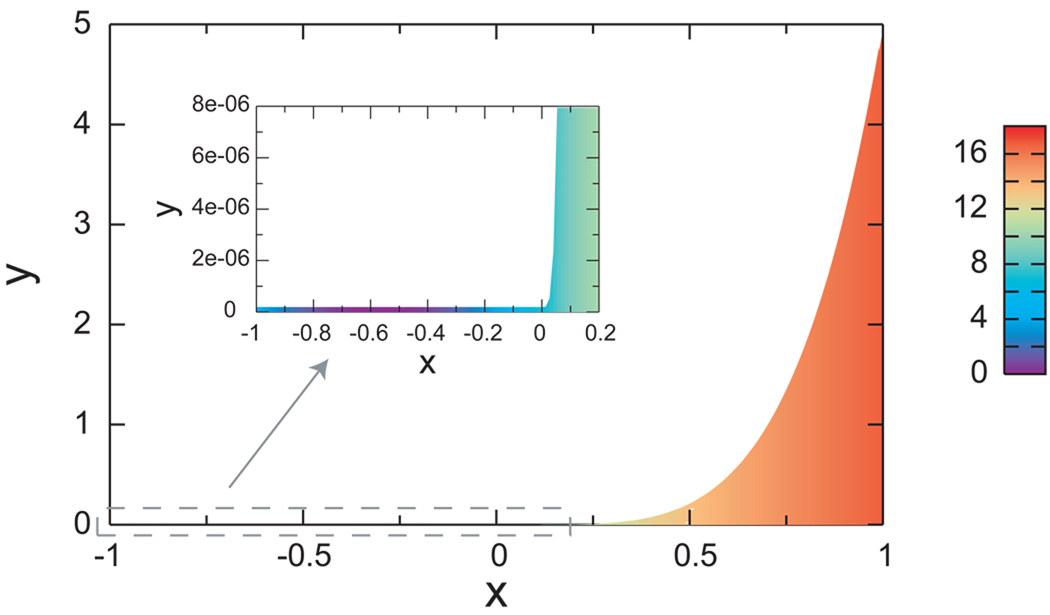
We use a two-dimensional potential (Fig. 1) described previously,⁴⁴ which was constructed to mimic the anti-Arrhenius temperature dependence of the folding rates seen in proteins. This potential was designed to have an energetic barrier when going from the “folded” (x < 0) to the “unfolded” (x ≥ 0) region, and an entropic barrier in the reverse direction. The entropic barrier is achieved by imposing a hard wall constraint that limits the space accessible to the folded region. Specifically the particle can only move in the region −1 ≤ x ≤ 1, 0 ≤ y ≤ B(x), where the boundary function B(x) is a small constant for x ≤ 0 and an increasing function of x for x > 0

$$B(x)=\{\begin{array}{cc}\delta \hfill & 1\le x\le 0\hfill \\ {\mathit{\text{bx}}}^{n_1}+\delta \hfill & 0<x\le 1\hfill \end{array}$$ (1)

where, for this study, δ = 2 × 10⁻⁷, b = 5 and n₁ = 4.55. Within this region, the potential energy is given by

$$U(x,y)=\{\begin{array}{ccc}{a}_1{(x+x_0)}^2,\hfill & \hfill -1\le x<-x_1\hfill & 0\le y\le B(x)\hfill \\ -a_2{x}^2+c_0,\hfill & \hfill -x_1\le x\le 0,\hfill & 0\le y\le B(x)\hfill \\ a_3{x}^2+c_{0,}\hfill & \hfill 0<x<x_2,\hfill & 0\le y\le B(x)\hfill \\ a_4{x}^{1/2}+c_1\hfill & \hfill x_2\le x\le 1,\hfill & 0\le y\le B(x)\hfill \\ \infty \hfill & \hfill \text{otherwise}\hfill & \hfill \end{array}$$ (2)

where a₁ = 23.53 kcal/mol, a₂ = 235.3 kcal/mol, a₃ = 376.5 kcal/mol, a₄ = 11.29 kcal/mol, and c₀ = 7.059 kcal/mol. The dimensionless constants x₀ = 0.5745, x₁ = 0.05222, x₂ = 0.03830, and the energy offset c₁ = 5.402 kcal/mol were chosen so that U(x, y) and its first derivative are continuous. With these parameters, the two-dimensional model has a folding rate with strong anti-Arrhenius temperature dependence, as well as Arrhenius behavior for the unfolding rates in the temperature range studied.

Figure 1.

A schematic representation of the two-dimensional potential function used here. The colored area corresponds to the accessible region of the (x, y) plane, with the colors representing the magnitude of the potential energy at that (x, y) point (scale bar in kcal/mol). The potential energy is infinite in the non-colored region and for y < 0, x < −1, and x > 1. The inset is an enlarged view of the folded macrostate and transition region.

We use Metropolis MC sampling⁴⁵ to simulate the movement of a particle in the potential. Because of the large size difference of the accessible region in the y direction between the folded and unfolded regions, we adopted an asymmetric Metropolis-Hastings or “smart MC” proposal scheme.^43,46,47 The step size in the y direction varies with B(x), i.e. a proposed move (Δx′, Δy′) is generated uniformly in the region −Δ < Δx′ < Δ, −B(x)Δ < Δy′ < B(x)Δ, where Δ = 0.01 is a constant for all temperatures. To correct for the asymmetric MC proposal distribution, the Metropolis acceptance probability was multiplied by θ(|y′ − y|/B(x)Δ) to satisfy detailed balance, where θ(z) equals 1 if z < 1 and 0 otherwise.

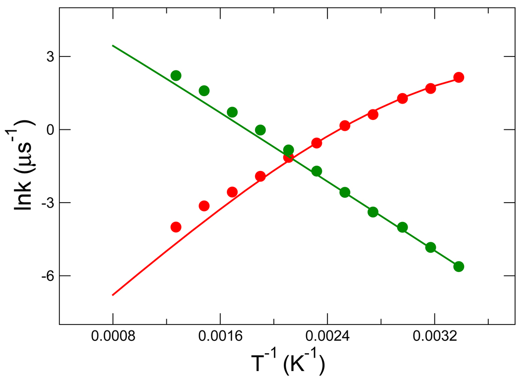
Rate constants were obtained via MC simulation by calculating the mean first passage times (MFPTs) in units of MC steps between the two macrostates. A “buffer region” −0.1 < x < 0.0437 was defined as not belonging to either the folded or unfolded macrostate to reduce artefactual rapid recrossings of the barrier. As discussed previously,⁴⁴ the folding rate has “anti-Arrhenius” behavior, i.e. it decreases as temperature increases, as shown in Fig. 2. Our goal is to reproduce this temperature dependence of the folding and unfolding rate using a kinetic network model.

Figure 2.

The temperature dependence of the folding and unfolding rate constants. Folding and unfolding rates are indicated by red and green, respectively. The rate constants indicated by circles were derived from kinetic MC simulations run at different temperatures. The lines represent the rates calculated using the Arrhenius equation based on activation energies derived from the PMF along x. Rate constants are expressed in units of 10⁻⁶ per MC step.

The network model is composed of nodes each representing a microstate of the system, which in this case is a point (x, y) in 2D space. We assume that the transition away from a given point along the x coordinate is a diffusive process locally described by a Fokker-Planck equation of the form:

$$\frac{\partial P(x,t)}{\partial t}=-\frac{\partial }{\partial x}[v(x)P(x,t)]+\frac{{\partial }^2}{\partial x^2}[D(x)P(x,t)]$$ (3)

where P(x, t) is the probability density of finding the particle at x at time t, and v(x) and D(x) are, respectively, the drift velocity and diffusion constant at x. In this work v(x) and D(x) are estimated from the rate of change of the mean x̄(t) and variance σ²(t) of the distribution of points obtained from a series of MC trajectories of length t started from points (x, y) at constant x

$$v(x)={\frac{\partial \overline{x}(t)}{\partial t}|}_{t=t^{*}}$$ (4)

and

$$D(x)={\frac{1}{2}\frac{\partial {\sigma }^2(t)}{\partial t}|}_{t=t^{*}},$$ (5)

where t* is sufficiently large to estimate the quantities of interest, but small enough so that it still represents the point of interest x. In practice, v(x) and D(x) are computed by fitting a straight line to x̄(t) and σ²(t) as a function of t. The interval we used for fitting is 5 MC steps. It is large enough to include 5 data points and still small enough so that the fit of the parameters is linear to a good approximation. Our goal is to build up a network with kinetics that mimics the local drift velocity and diffusion constant of the MC simulation of the system on the continuous potential.

2.2 Construction of the kinetic network model

2.2.1 Discretization of the state space

The nodes of the kinetic network are a discretized approximation of the original state space of the system. We ran a replica exchange Monte Carlo (REMC) simulation on the two-dimensional potential with S = 8 replicas at temperatures ranging from 296 K to 789 K for 10⁹ MC steps. Every 1000 MC steps, transitions between two adjacent temperatures were attempted. Immediately before attempting temperature exchanges, the configuration of each replica was stored, obtaining N = 50, 000 configurations at each temperature, and N × S = 400, 000 configurations at all temperatures. This ensemble of conformations constitutes the discretized state space of the system, which, as described below, approximates well the equilibrium thermodynamics of the system for any temperature within the simulated temperature range or not too far above or below the range.

Traditionally, equilibrium thermodynamic properties of the system at temperature T₀ are obtained by performing canonical sampling at T₀ for a long enough time to obtain convergence. We and others have shown^39,43 that improved convergence can be achieved by employing T-WHAM on RE trajectories over a range of temperatures (which need not include T₀). This yields canonical ensemble averages with greater efficiency than traditional sampling methods because it combines data from high temperature replicas, which sample high energy and high entropy regions, and data from low temperature replicas, which preferentially sample low energy, low entropy regions. The T-WHAM approach is based on a re-weighting scheme designed to minimize statistical error.⁴³ The T-WHAM canonical average 〈A(T₀)〉 of a quantity A at temperature T₀ is

$$\langle A(T_0)\rangle ={\displaystyle \sum _{i=1}^N{w}_i(T_0)A_i,}$$ (6)

where the summation runs over the N RE conformations from all temperatures, A_i is the value of A for conformation i, and the weight factor w_i(T₀) is given by^48,49

$$w_i(T_0)={\left\{{\displaystyle \sum _{k=1}^S{N}_k{f}_k\text{ exp }\left[\left(\frac{1}{k_b{T}_0}-\frac{1}{k_b{T}_k}\right)E_i\right]}\right\}}^{-1},$$ (7)

where N_k is the number of samples at each of the S different replica exchange temperatures T_k, and k_b is the Boltzmann constant. The natural logarithms of the constants f_k in Eq. 7 correspond to the relative Helmholtz free energy of each replica k such that f_k/f_k′ = Q_k/Q_k′, where Q_k is the canonical partition function of the system at temperature T_k. In T-WHAM the f_k’s are determined by iteratively solving a system of non-linear equations known as the WHAM equations.^43,48 Thus, each sample i has a weight factor associated with it (Eq. 7) that depends only on its energy E_i and the temperature of interest T₀. To calculate the PMF of the system as a function of x at temperature T₀ using the discretized state space, it is sufficient to employ Eq. 6 with A being an indicator function which is non-zero if the x-coordinate of the sample is near the designated value of x. This can be done for any temperature T₀, which need not be one of the temperatures used in the RE simulations.

2.2.2 Thermodynamics of the network model

To complete the specification of the kinetic network model, we must provide a network topology in the form of edges which connect the nodes and microscopic rates associated with each edge. The choices made for these parameters will determine the kinetics of the network, however, they will not affect the equilibrium thermodynamics of the network as long as detailed balance is satisfied (see Eq. 8 below) and the network topology is ergodic (i.e. any node is accessible from any other in a finite number of edge traversals). How well the equilibrium properties of the network approximate the real equilibrium thermodynamics of the system depends on the quality of the discretization of the state space using RE.

We connect two nodes with an edge if they are “close” in Euclidean space. Specifically, we join nodes corresponding to coordinates (x, y) and (x′, y′) if |x′ − x| < Δ_x and |y′ − y| < Δ_y. We have chosen the cut-off lengths Δ_x and Δ_y to be much smaller than the dimensions of the system so as to appropriately mimic the local nature of the continuous MC kinetics (see below). We then assign forward and reverse rates to each edge so that detailed balance is satisfied. For example, if nodes i and j are connected by an edge, then we choose rates k_ij(T) and k_ji(T) such that

$$\frac{k_{\mathit{\text{ij}}}(T)}{k_{\mathit{\text{ji}}}(T)}=\frac{w_i(T)}{w_j(T)},$$ (8)

where w_i(T) and w_j(T) are the weight factors of the two nodes at temperature T, k_ij(T) is the rate going from node i to node j, k_ji(T) is the reverse rate. If this detailed balance condition is satisfied, the asymptotic thermodynamics produced by the network model will be the same as that of the original system (subject to the aforementioned ergodicity criterion).

We simulate the kinetics on this network as a continuous time Markov process with discrete states using the Gillespie Algorithm.⁵⁰ During the simulation, the population histogram along the x coordinate (the reaction coordinate for our two-dimensional system) was accumulated. When a node is visited, its residence time is added to the corresponding bin in the histogram and at the end of the simulation, the histogram is used to calculate the PMF along the x coordinate.

2.2.3 Calibration of the kinetic properties of the network model

Although the network design strategy described above guarantees that the correct thermodynamic properties are reproduced, the ability to reproduce the correct kinetics requires additional considerations. Information about the local dynamics of the system in some form is required to obtain a kinetically realistic network. In this section we illustrate how this can be done for the case of a two-dimensional potential system, where we reproduce the kinetics of a MC simulation on the continuous potential with a network model.

For kinetic MC simulations, the “time” unit is the MC step. The kinetics depends on the move set, which in our case was the box defined by the intervals [−Δ, Δ] and [−10B(x)Δ, 10B(x)Δ] for x and y, respectively, and where Δ = 0.01. Note that the magnitude of the allowed moves in the y direction is not constant, but depends on x and varies with the size B(x) of the accessible region in the y direction. To recover the kinetics of the MC simulation on the continuous potential, we choose a network topology that mimics the MC move set, as described in the Appendix.

To assign microscopic rates to the edges that satisfy detailed balance, we could choose

$$k_{\mathit{\text{ij}}}(T)=\frac{w_j(T)}{w_i(T)}{\mu }_{\mathit{\text{ij}}}$$ (9)

and

$$k_{\mathit{\text{ji}}}(T)={\mu }_{\mathit{\text{ij}}}$$ (10)

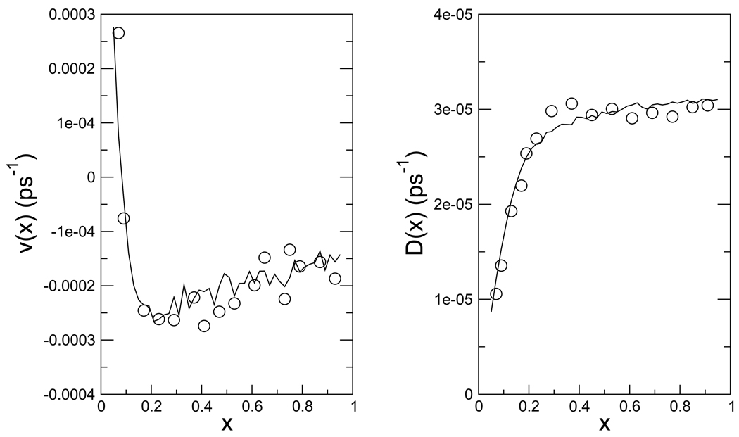
where μ_ij = μ_ji is a base rate to be determined for each pair of nodes i and j to obtain the best agreement with the observed MC kinetics on the continuous potential. To find the appropriate base rates μ_ij to match the drift velocity and diffusion coefficients of the network simulation with that of the kinetic MC, we ran 10,000 short trajectories (5–10 MC steps) starting at different values of x with both the kinetic MC simulations on the continuous potential and Gillespie simulations on the discretized network model to evaluate the local drift velocities and diffusion coefficients as a function of x. The results are shown in Fig. 3.

Figure 3.

The drift velocity v(x) and diffusion coefficient D(x) along the reaction coordinate x at 298 K. The lines represent the drift velocity and diffusion coefficient of the kinetic MC simulation on the continuous potential, while the circles are the results from the discretized kinetic network model after calibration of c₀.

For the two-dimensional test case studied here, the appropriate values of μ_ij are those which allow the network simulation to most closely replicate kinetic MC. In other words, we would like a “time unit” in the Gillespie algorithm to correspond to an MC step in the kinetic MC. In the latter case, each transition between microstates corresponds to an elapsed “time” of 1 unit. Since the edges of the network which join microstates have already been chosen to mimic the kinetic MC move set, it remains only to ensure that the average time between microstate transitions in the discrete network simulation also corresponds to 1 time unit.

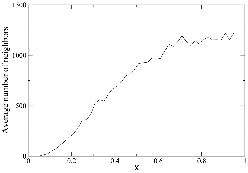
In the Gillespie algorithm, the average waiting time in a node is inversely proportional to the sum of the microscopic rates exiting the node. The waiting time in a given node is approximately proportional to the inverse of the number of neighbors for the node, given the fact that the neighbors are close in Euclidean space and have similar energies and similar weights. Therefore, the corresponding edges will have similar rates according to Eq. 9. As seen in Fig. 4, the average number of neighbors for a node increases with x due to the bigger cut-off length in y direction used to define network edges. Thus, the average waiting time between transitions among microstates will be shorter for nodes with large x. The proportionality between MC steps and Gillespie time units can be maintained by setting μ_ij = c₀/n_ij, where c₀ is an adjustable coefficient, and n_ij is the average number of neighbors for the connected nodes i and j. The 1/n_ij factor in the rate ensures that the waiting times in all nodes are of similar magnitude. We use the average of the number of neighbors for the two connected nodes and not the number of neighbors of the current node, since the latter would violate detailed balance if the current and successor nodes have different numbers of neighbors. It should be noted that this strategy for determining μ_ij amounts to making the Gillespie algorithm mimic kinetic MC on the continuous potential, and different but analogous approaches would be needed for Newtonian dynamics on a high-dimensional potential.

Figure 4.

The average number of neighbors per node for all nodes which have a given value of the reaction coordinate x.

3 Results and Discussion

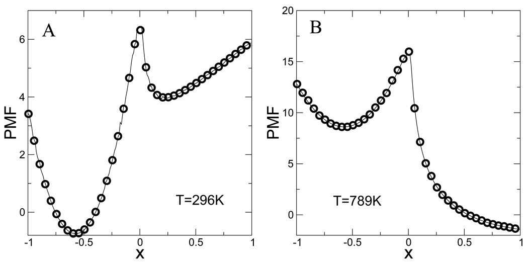
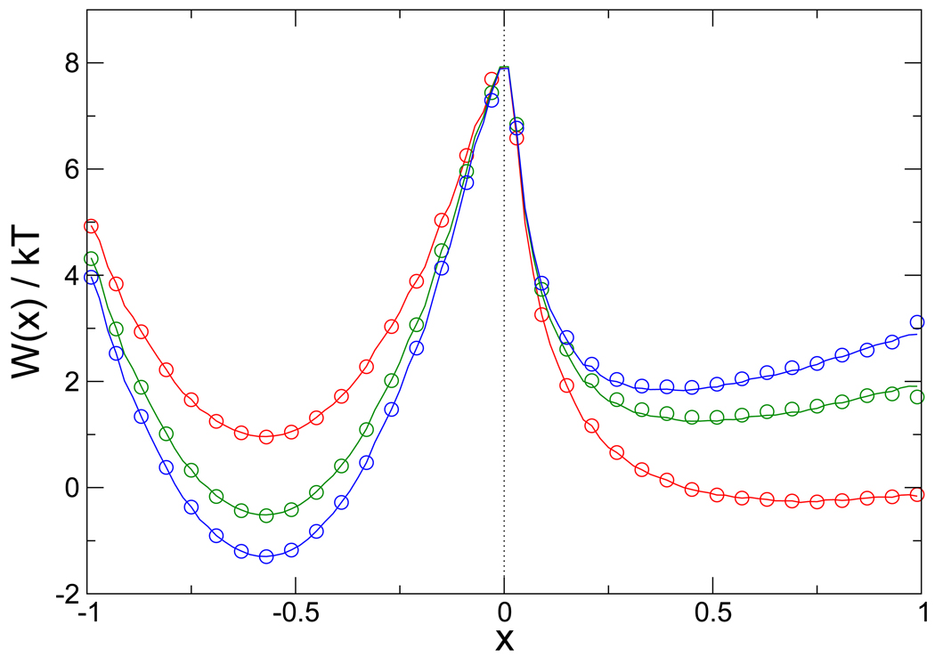
To confirm that the 400, 000 configurations generated using replica exchange MC on the two-dimensional continuous potential give the correct thermodynamic behavior, we compared the PMFs along the x coordinate at several temperatures calculated from the discretized state space and the weight factors of Eq. 7 with the one calculated by numerical integration of the canonical distribution function of this system. The agreement is excellent at all temperatures examined (only the highest and lowest temperatures are shown in Fig. 5 for clarity). This indicates that the correctly weighted discretized state space is a good approximation to the PMF on the continuous potential at all the temperatures studied. Excellent agreement for the PMF is also obtained from Gillespie simulations using the network model with a generic network topology and rate parameters (Δ = 0.01, and μ_ij = 1 for all i, j), as shown in Fig. 6. This validates the implementation of the network model algorithm, and indicates that the ergodicity condition is satisfied.

Figure 5.

The PMF at two different temperature 296 K and 789 K. Solid lines are the exact value calculated by numerical integration of the potential. Circles are derived from the full ensemble of 8 temperatures combined using WHAM.

Figure 6.

The PMF along the x coordinate at the three temperatures 395 K, 431 K, and 526 K (blue, green, and red, respectively). Solid lines are the exact PMFs calculated by numerical integration of the potential, while the circles are derived from kinetic network simulations at each temperature. Approximately 10³ barrier crossings were observed in the 1 hour of wall clock time required for each simulation.

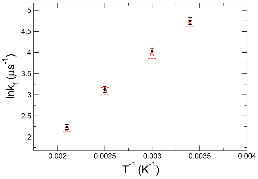
We ran a series of short time trajectories using both kinetic MC on the continuous potential and Gillespie dynamics on the discretized network model, and evaluated the drift velocities and diffusion coefficients along the reaction coordinate at different x positions. By varying the parameters of the network in order to match the drift and diffusion on the network with that of the kinetic MC simulation on the the conditional potential, we obtained optimized rate parameters for the network model. We made use of the choice of μ_ij described above and adjusted c₀ by grid search to optimize the agreement of the drift velocities in the kinetic network model and the kinetic MC. The drift velocities were chosen as the target of the optimization, since it showed the stronger dependence on c₀. We found that c₀ = 0.85 at T₀ = 298 K (for all x) gives good agreement, as shown in Fig. 3. Furthermore, the folding rates at different temperatures obtained from MC simulations on the continuous potential and from the discretized kinetic network simulation agree very well, as shown in Fig. 7.

Figure 7.

Arrhenius plot of the folding rates of the model system. The solid symbols represent the folding rate from kinetic MC simulations on the continuous potential in unit of 10⁻⁶ per MC step. The open circles represent the rates from simulations of the discretized kinetic network model. The error bars represent one standard deviation, as estimated by error propagation from the first passage time distribution. Solid and dashed error bar lines correspond to the results of kinetic MC and network model, respectively.

The results (Fig. 7) demonstrate that for the two-dimensional model system for protein folding studied here, it is possible to reconstruct the folding kinetics on a continuous potential using a discrete network model of the type used by Andrec, et al.⁴² This network model employed an ad hoc method for assigning weights to nodes from different simulation temperatures, while the present model uses weights based on the firm statistical mechanical footing of the T-WHAM method.⁴³ In fact, the present formulation for the model system studied here reproduces the exact PMFs obtained from numerical integration. This result is general, in that we can expect to obtain PMFs consistent with the RE simulation and T-WHAM without the need for any special choice of reduced coordinate. This is because the f_k factors which appear in Eq. 7 are directly related to the free energies associated with a given replica. While the WHAM equations themselves require a choice of reduced coordinate which one uses to construct the histograms, the resulting f_k factors do not depend on that choice. Correspondingly, although our local dynamic parameters are estimated on a reduced coordinate, the actual kinetic simulation does not occur on that reduced coordinate, but rather on the full network, which, by including virtually all degrees of freedom, allows for multiple pathways and transition states.

The model system studied here is sufficiently simple that we can fully confirm the validity of our approach, but is of course much simpler than any atomic-level molecular model. There is then the question of the applicability of this methodology to such systems. Previous studies^9–14 have shown that it is possible to capture the local kinetics of complex molecular systems using a limited number of degrees of freedom. Concomitantly, we have shown that discrete network models⁴² can yield physically plausible pathways for protein folding. Taken together, these observations indicate that the methodology described here will likely be useful to model the kinetics of complex molecular systems.

Nonetheless, the practical implementation of this methodology will require a careful consideration of the additional complexities involved. For example, the large dimensionality of molecular systems may make it difficult to find good reduced coordinates with respect to which local kinetics could be obtained. Since we only require a well-defined measure of local kinetics, we are not limited to methods based on the Fokker-Planck equation (Eq. 3). For example, one could make use of conformational clustering to define local neighborhoods, and then measure within-cluster and between-cluster dynamics using both local dynamics simulations and the kinetic network. The parameters of the network can then be adjusted to optimize the match. Alternatively, local dynamics could be modeled along appropriate generalized coordinates, or the calibration of the network model parameters could be done using kinetic properties that do not depend on a reaction coordinate.

A second layer of complexity that will be involved in application of this methodology to larger systems arises in the adjustment of the network in order to reproduce local dynamics. In the model described above, the choice of network topology (the number of edges and which nodes which they connect) was straightforwardly dictated by the move set of the kinetic scheme MC we were trying to reproduce. Furthermore, because this structure was independent of target temperature, we assumed that the parameter c₀ could be taken to be a constant for all nodes and all temperatures. In a molecular system, these parameters will likely need to be varied, and the determination of the optimal network parameters may require a multidimensional search over topology and rate parameters μ_ij.

4 Conclusions

In this paper we have presented a novel kinetic network strategy for the study of slow time scale processes that extends and improves our previous approach.⁴² We use RE simulation and T-WHAM to generate a large set of discrete states with correct thermodynamics. A kinetic network is constructed using the discrete states as nodes using weights that preserve these populations. The microscopic rates between each pair of nodes are calibrated to insure local dynamics consistent with those of the full system. The dynamics on the calibrated network is then simulated to study the long timescale kinetics of the system. We have tested the validity of the methods on a two-dimensional continuous potential with anti-Arrhenius kinetics. Application of the kinetic network model to more complex peptide or protein systems will reveal not only high-dimensional kinetic pathways, but also will allow us to estimate quantities such as P_fold ⁵¹ to acquire information about the transition states of the slow process.

Our method differs from previous approaches which decompose the configurational space into a relative small number of metastable macrostates or project the kinetics onto a chosen reaction coordinate.^13,14,30,52 Our approach does not rely on finding a good reaction coordinate. We compute local stochastic dynamical quantities on a reduced coordinate, but only as a benchmark to calibrate the parameters of a network model constructed from the full discretized state space of the system. The manner in which this calibration is performed can be tailored to the specific demands of the system being studied, and the quantities used for calibration need not be structural coordinates. After calibration, the kinetic simulations are performed on the full network representing a discretization of the high-dimensional state space. This allows for multiple reaction pathways, and allows us the flexibility to analyze the dynamics using reduced coordinates of our choosing.

The network model is a Markovian model, like that of other previous approaches,^17–20,32 but instead of using artificially defined macrostates, we use a large number of microstates collected from a RE simulation of the system. This increases the chances of constructing a realistic picture of the kinetics, at the cost of a larger and more complex network. The computational cost of the Gillespie Algorithm to perform a single jump between a node and one of its N neighbors scales as O(logN) in our implementation. From past experience,⁴² a much larger network with ≈ 10⁶ states and > 10⁹ edges is still manageable with current computational resources. Since all configurations are precalculated, there is a much lower computational burden than for a comparable all-atom simulation, since (for example) potential energies and forces do not need to be evaluated. If necessary, methods for accelerating Gillespie-type simulations that have been developed in the context of chemical reaction and systems biology simulations could be used to mitigate the computational burden.⁵³ We believe that the kinetic network method demonstrated here will be a useful addition to the arsenal of computational methods for the study of slow processes in complex molecular systems.

Appendix

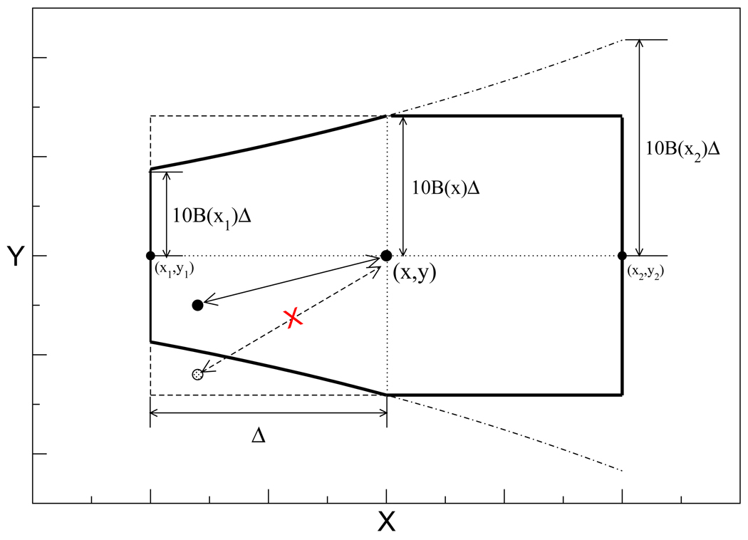
The goal of designing the kinetic network model is to provide the best possible agreement with the kinetic MC simulation on the two-dimensional continuous potential. This goal is more likely to be met if the structure of the network closely mimics the structure of the move set which underlies the kinetic MC. One key choice in the design of the kinetic network is its topology, i.e. which pairs of nodes are to be connected by edges. In previous work,⁴² we used a simple “box” rule that placed an edge if two nodes were sufficiently close in configuration space. In the case of the MC kinetic scheme used for the two-dimensional potential here, a better choice would more closely mimic the asymmetry of the particular move set used in the MC simulation. In Fig. 8 we show the region that a particle starting from a point (x, y) can access and return in two successive MC steps. It consists of the square region excluding the two corners on the left: although the particle could reach the left corners in one step, it is impossible for it to come back to (x, y) in one step. Therefore in the network model, we also exclude the corresponding node pairs and construct edges only between nodes that satisfy either of the two conditions

$$\begin{array}{ccc}x-\mathrm{\Delta }<x^{\prime }<x\hfill & \text{and}\hfill & |y-y^{\prime }|<10B(x^{\prime })\mathrm{\Delta }\hfill \\ x<x^{\prime }<x+\mathrm{\Delta }\hfill & \text{and}\hfill & |y^{\prime }-y|<10B(x)\mathrm{\Delta }.\hfill \end{array}$$ (11)

Figure 8.

Diagram illustrating the neighboring pair rule for the network model, showing the locus of points (region within the solid line) that can be reversibly visited from a given reference point (x, y). B(x) is the function that defines the accessible region of the system, Δ is the maximum MC step size, x₁, y₁, x₂, y₂ correspond to the coordinates of the most distant points reachable from (x, y) in one MC step. The dashed-dotted line encloses the area accessible in one MC move from (x, y). The dashed line is a rectangle around (x, y) of dimensions Δ and 10B(x)Δ along the x and y axes, respectively,

References

- 1.Onuchic JN, Wolynes PG. Curr. Opinion Struct. Biol. 2004;14:70–75. doi: 10.1016/j.sbi.2004.01.009. [DOI] [PubMed] [Google Scholar]
- 2.Elber R. Curr. Opinion Struct. Biol. 2005;15:151–156. doi: 10.1016/j.sbi.2005.02.004. [DOI] [PubMed] [Google Scholar]
- 3.Snow CD, Sorin EJ, Rhee YM, Pande VS. Ann. Rev. Biophys. Biomol. Struct. 2005;34:43–69. doi: 10.1146/annurev.biophys.34.040204.144447. [DOI] [PubMed] [Google Scholar]
- 4.Christen M, van Gunsteren WF. J. Comput. Chem. 2007;29:157–166. doi: 10.1002/jcc.20725. [DOI] [PubMed] [Google Scholar]
- 5.Bolhuis PG, Chandler D, Dellago C, Geissler PL. Annu. Rev. Phys. Chem. 2002;53:291–318. doi: 10.1146/annurev.physchem.53.082301.113146. [DOI] [PubMed] [Google Scholar]
- 6.Zagrovic B, Sorin EJ, Pande V. J. Mol. Biol. 2001;313:151–169. doi: 10.1006/jmbi.2001.5033. [DOI] [PubMed] [Google Scholar]
- 7.Pande VS, Baker I, Chapman J, Elmer SP, Khaliq S, Larson SM, Rhee YM, Shirts MR, Snow CD, Sorin EJ, Zagrovic B. Biopolymers. 2003;68:91–109. doi: 10.1002/bip.10219. [DOI] [PubMed] [Google Scholar]
- 8.Faradjian AK, Elber R. J. Chem. Phys. 2004;120:10880. doi: 10.1063/1.1738640. [DOI] [PubMed] [Google Scholar]
- 9.Schumaker MF, Pomès R, Roux B. Biophys. J. 2000;79:2840–2857. doi: 10.1016/S0006-3495(00)76522-2. [DOI] [PMC free article] [PubMed] [Google Scholar]
- 10.Hummer G, Kevrekidis IG. J. Chem. Phys. 2003;118:10762. [Google Scholar]
- 11.Kopelevich DI, Panagiotopoulos AZ, Kevrekidis IG. J. Chem. Phys. 2005;122:044908. doi: 10.1063/1.1839174. [DOI] [PubMed] [Google Scholar]
- 12.Best RB, Hummer G. Phys. Rev. Lett. 2006;96:228104. doi: 10.1103/PhysRevLett.96.228104. [DOI] [PubMed] [Google Scholar]
- 13.Yang S, Onuchic JN, Levine H. J. Chem. Phys. 2006;125:054910. doi: 10.1063/1.2229206. [DOI] [PubMed] [Google Scholar]
- 14.Yang S, Onuchic JN, Garcìa AE, Levine H. J. Mol. Biol. 2007;372:756–763. doi: 10.1016/j.jmb.2007.07.010. [DOI] [PubMed] [Google Scholar]
- 15.Berezhkovskii A, Szabo A. J. Chem. Phys. 2005;122:014503. doi: 10.1063/1.1818091. [DOI] [PubMed] [Google Scholar]
- 16.Ozkan SB, Dill KA, Bahar I. Protein Sci. 2002;11:1958–1970. doi: 10.1110/ps.0207102. [DOI] [PMC free article] [PubMed] [Google Scholar]
- 17.Ye Y-J, Ripoll DR, Scheraga HA. Comp. Theor. Polymer Sci. 1999;9:359–370. [Google Scholar]
- 18.Singhal N, Snow CD, Pande VS. J. Chem. Phys. 2004;121:415–425. doi: 10.1063/1.1738647. [DOI] [PubMed] [Google Scholar]
- 19.Swope WC, Pitera JW, Suits F. J. Phys. Chem. B. 2004;108:6571–6581. [Google Scholar]
- 20.Swope WC, Pitera JW, Suits F, Pitman M, Eleftheriou M, Fitch BG, Germain RS, Rayshubski A, Ward TJC, Zhestkov Y, Zhou R. J. Phys. Chem. B. 2004;108:6582–6594. [Google Scholar]
- 21.Noé F, Horenko I, Schütte C, Smith JC. J. Chem. Phys. 2007;126:155102. doi: 10.1063/1.2714539. [DOI] [PubMed] [Google Scholar]
- 22.Rogal J, Bolhuis PG. J. Chem. Phys. 2008;129:224107. doi: 10.1063/1.3029696. [DOI] [PubMed] [Google Scholar]
- 23.Voter AF. Phys. Rev. B. 1998;57:R13985–R13988. [Google Scholar]
- 24.Shirts MR, Pande VS. Phys. Rev. Lett. 2001;86:4983–4987. doi: 10.1103/PhysRevLett.86.4983. [DOI] [PubMed] [Google Scholar]
- 25.Ma A, Dinner AR. J. Phys. Chem. B. 2005;109:6769–6779. doi: 10.1021/jp045546c. [DOI] [PubMed] [Google Scholar]
- 26.Krivov SV, Karplus M. J. Phys. Chem. B. 2006;110:12689–12698. doi: 10.1021/jp060039b. [DOI] [PubMed] [Google Scholar]
- 27.Krivov SV, Muff S, Caflisch A, Karplus M. J. Phys. Chem. B. 2008;112:8701–8714. doi: 10.1021/jp711864r. [DOI] [PMC free article] [PubMed] [Google Scholar]
- 28.Rao F, Caflisch A. J. Mol. Biol. 2004;342:299–306. doi: 10.1016/j.jmb.2004.06.063. [DOI] [PubMed] [Google Scholar]
- 29.Schultheis V, Hirschberger T, Carstens H, Tavan P. J. Chem. Theory Comput. 2005;1:515–526. doi: 10.1021/ct050020x. [DOI] [PubMed] [Google Scholar]
- 30.Chodera JD, Singhal N, Pande VS, Dill KA, Swope WC. J. Chem. Phys. 2007;126:155101. doi: 10.1063/1.2714538. [DOI] [PubMed] [Google Scholar]
- 31.Chekmarev DS, Ishida T, Levy RM. J. Phys. Chem. 2004;108:19487–19495. [Google Scholar]
- 32.Buchete N-V, Hummer G. Phys. Rev. E. 2008;77:030902. doi: 10.1103/PhysRevE.77.030902. [DOI] [PubMed] [Google Scholar]
- 33.Wei G, Mousseau N, Derreumaux P. Proteins. 2004;56:464–474. doi: 10.1002/prot.20127. [DOI] [PubMed] [Google Scholar]
- 34.Evans DA, Wales DJ. J. Chem. Phys. 2004;121:1080–1090. doi: 10.1063/1.1759317. [DOI] [PubMed] [Google Scholar]
- 35.Wales DJ. Mol. Phys. 2002;100:3285–3305. [Google Scholar]
- 36.Carr JM, Wales DJ. J. Phys. Chem. B. 2008;112:8760–8769. doi: 10.1021/jp801777p. [DOI] [PubMed] [Google Scholar]
- 37.Krivov SV, Karplus M. Proc. Natl. Acad. Sci. USA. 2004;101:14766–14770. doi: 10.1073/pnas.0406234101. [DOI] [PMC free article] [PubMed] [Google Scholar]
- 38.Mitsutake A, Sugita Y, Okamoto Y. Biopolymers. 2001;60:96–123. doi: 10.1002/1097-0282(2001)60:2<96::AID-BIP1007>3.0.CO;2-F. [DOI] [PubMed] [Google Scholar]
- 39.Sugita Y, Okamoto Y. Chem. Phys. Lett. 1999;314:141–151. [Google Scholar]
- 40.Zheng W, Andrec M, Gallicchio E, Levy RM. Proc. Natl. Acad. Sci. USA. 2007;104:15340–15345. doi: 10.1073/pnas.0704418104. [DOI] [PMC free article] [PubMed] [Google Scholar]
- 41.van der Spoel D, Seibert MM. Phys. Rev. Lett. 2006;96:238102. doi: 10.1103/PhysRevLett.96.238102. [DOI] [PubMed] [Google Scholar]
- 42.Andrec M, Felts AK, Gallicchio E, Levy RM. Proc. Natl. Acad. Sci. USA. 2005;102:6801–6806. doi: 10.1073/pnas.0408970102. [DOI] [PMC free article] [PubMed] [Google Scholar]
- 43.Gallicchio E, Andrec M, Felts AK, Levy RM. J. Phys. Chem. B. 2005;109:6722–6731. doi: 10.1021/jp045294f. [DOI] [PubMed] [Google Scholar]
- 44.Zheng W, Andrec M, Gallicchio E, Levy RM. J. Phys. Chem. B. 2008;112:6083–6093. doi: 10.1021/jp076377+. [DOI] [PMC free article] [PubMed] [Google Scholar]
- 45.Metropolis N, Rosenbluth AW, Rosenbluth MN, Teller AH, Teller E. J. Chem. Phys. 1953;21:1087–1091. [Google Scholar]
- 46.Hastings WK. Biometrika. 1970;57:97–109. [Google Scholar]
- 47.Allen MP, Tildesley DJ. Computer Simulation of Liquids. Oxford: Oxford University Press; 1987. [Google Scholar]
- 48.Kumar S, Bouzida D, Swendsen RH, Kollman PA, Rosenberg JM. J. Comp. Chem. 1992;13:1011–1021. [Google Scholar]
- 49.Shirts MR, Chodera JD. J. Chem. Phys. 2008;129:124105. doi: 10.1063/1.2978177. [DOI] [PMC free article] [PubMed] [Google Scholar]
- 50.Gillespie DT. Markov Processes An Introduction for Physical Scientists. Boston: Academic Press; 1992. [Google Scholar]
- 51.Du R, Pande VS, Grosberg AY, Tanaka T, S.Shakhnovich E. J. Chem. Phys. 1998;108:334–350. [Google Scholar]
- 52.Chodera JD, Swope WC, Pitera JW, Dill KA. Multiscale Model. Simul. 2006;5:1214–1226. [Google Scholar]
- 53.Gillespie DT. Annu. Rev. Phys. Chem. 2007;58:35–55. doi: 10.1146/annurev.physchem.58.032806.104637. [DOI] [PubMed] [Google Scholar]