Diffeomorphic Sulcal Shape Analysis for Cortical Surface Registration

Abstract

We present an intrinsic framework for constructing sulcal shape atlases on the human cortex. We propose the analysis of sulcal and gyral patterns by representing them by continuous open curves in ℝ³. The space of such curves, also termed as the shape manifold is equipped with a Riemannian L² metric on the tangent space, and shows desirable properties while matching shapes of sulci. On account of the spherical nature of the shape space, geodesics between shapes can be computed analytically. Additionally, we also present an optimization approach that computes geodesics in the quotient space of shapes modulo rigid rotations and reparameterizations. We also integrate the elastic shape model into a surface registration framework for a population of 176 subjects, and show a considerable improvement in the constructed surface atlases.

1. Introduction

The cerebral cortex in mammalian brains is largely responsible for memory, thought processes, and sensory perceptions, and plays a key role in social abilities, language development, and abstract reasoning and thought, especially in human brains. The cortex comprises of neurons and nerve fibers and appears gray in color. The boundary of this gray matter region, also referred to as the cortical surface, can be observed as a highly convoluted exterior with valleys (sulci) and ridges (gyri). Cortical surfaces among populations exhibit highly varied folding patterns and it is of great interest to neuroscientists as well as neurologists to recognize, classify, and understand them. A surface-based morphometric analysis of the cortex is shown to have wide reaching applicability for the purpose of mental disease detection, progression, as well as prediction and understanding of normal and abnormal developmental behaviors. Surface-based morphometry has three major ingredients: i) representation of the cortical surface, ii) registration and alignment of one or more surfaces for construction of atlases, and iii) statistical analysis of deformations or warps explaining the variability of surface features in a given population. Surface registration aims at determining correspondences between a pair of surfaces by aligning several homologous features with respect to each other. The correspondence can be achieved either automatically, for e.g. using both local and global features as in the case of Fischl et al. [5, 2], or in a semi-automatedmanner, using expertly delineated sulcal and gyral landmarks as in the case of Thompson et al. [14, 7]. These landmarks are usually 3D continuous space curves corresponding to the deepest regions of the valleys for sulci, and topmost regions of the ridges for the gyri. Typically it is difficult for automated algorithms to locate, and classify sulcal and gyral patterns exclusively based on local geometric features. Thus the main advantage of using explicit landmarks is the incorporation of expert anatomical knowledge that improves the consistency in matching of homologous features. This in turn potentially improves statistical power in the neighborhood of the landmarks. Additionally, increasing the number of consistent landmarks also improves the alignment accuracy, thereby allowing more control in the registration process.

Previously, landmark curves have mostly been used as boundary conditions for various cortical alignment approaches. Their shapes have largely been ignored during registration. The sulcal and gyral fissures are highly correlated with the folding patterns of the cortex. Recently, there has been a renewed interest in studying the cortical folding patterns for the purpose of increased understanding of the organizational processes leading to the development of the cortex [4, 10, 3, 12]. Furthermore, the shapes of such patterns are also linked with brain function. In this paper we focus on modeling the shape of sulci and gyri, and incorporating it during the process of cortical registration and atlas construction. In the past, various researchers have modeled the sulci and gyri using different representations. Leow et al. [9] have demonstrated multiple curve comparison strategies that include homothetic mapping of curves discretized with equally spaced points, and whole-curve matching by relaxing point-wise correspondences between pairs of curves. However, they project three-dimensional sulcal geometry onto a two-dimensional plane, and then use diffeomorphic mappings between the flat planes to find point correspondences. Tao et al. [13] represent sulci using landmark points on curves, and build a statistical model by using a Procrustes alignment of sulcal shapes. Vaillant et al. [15] represent cortical sulci by medial surfaces of cortical folds. They subsequently parameterize the surface into salient isoparametric active contours. Although, the advantage of this model is that it represents entire cortical folds, a limitation of this method is the use of unit speed parameterizations of active contours for constructing Procrustes shape averages for sulci. This implies that the average shape is only invariant to translation, rotation, and scaling. Furthermore, for the latter two approaches, the shapes are represented by finite features or landmarks, and thus are limited in characterization of the rich geometric detail that manifests in the cortical folds that give the sulci their shapes.

1.1. Contributions

In this paper, unlike the previous approaches, we will represent the sulci and gyri by parameterized three-dimensional curves. Instead of analyzing the curves directly, we will deal with their functional representations that map curve instances onto a shape manifold. The main contributions of this paper are as follows:

1. An inverse-consistent diffeomorphic framework for matching sulcal shapes.

2. An intrinsic sulcal shape atlas based on the Riemannian metric on the shape manifold.

3. Integration of sulcal curve diffeomorphisms in driving cortical surface registrations.

To our knowledge, the proposed framework of direct diffeomorphic three-dimensional sulcal curve mappings have not been used in cortical registration before. Additionally, we also show comparisons of shape averages of our approach to the standard Euclidean curve matching that is normally used in surface registration.

The remainder of this paper is organized as follows. Section 2 outlines the shape modeling scheme for sulci and gyri. It deals with the shape representation, and specifies a Riemannian metric on the tangent space of the shape manifold. Section 3 outlines the procedure for computing statistical shape averages for sulci and gyri for a given population. Finally Section 4 incorporates the sulcal shape model in cortical surface registration, followed by results and conclusion.

2. Diffeomorphic Shape Analysis of Sulci and Gyri

In this section, we describe the modeling scheme used to represent sulcal and gyral shape features. We will represent the cortical valleys (sulci), and the ridges (gyri) by open curves. However unlike previous approaches which have used landmarks for representing the sulcal and gyral features, we will use continuous functions of curves for representing shapes. For example, Fig. 1 shows the lateral, medial and the ventral views of a cortical surface along with manually highlighted sulci and gyri.

Figure 1.

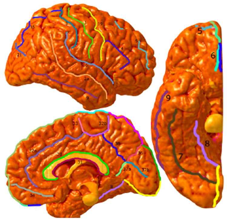
Cortical Surface with manually traced sulci and gyri.

2.1. Shape Representation

We use a vector valued map to parameterize the 3D sulci and gyri as follows. Let β be a 3D, arbitrarily parameterized, open curve, such that β : [0, 2π] → ℝ³. We represent the shape of the curve β by the function q : [0, 2π] → ℝ³ as follows,

$$q(s)=\frac{\dot{\beta }(s)}{\sqrt{\parallel \dot{\beta }(s)\parallel }}\in {\mathrm{ℝ}}^3.$$ (1)

Here, s ∈ [0, 2π], $\parallel ·\parallel \equiv \sqrt{(·,·){\mathrm{ℝ}}^3}$, and (·, ·)ℝ³ is taken to be the standard Euclidean inner product in ℝ³. The quantity ∥q(s)∥ is the square-root of the instantaneous speed, and the ratio $\frac{q(s)}{\parallel q(s)\parallel }$ is the instantaneous direction along the curve. The original curve β can be recovered upto a translation, using $\beta (s)={\mathit{\int }}_0^s\parallel q(t)\parallel q(t)\mathit{dt}$. In order to make the representation scale invariant, we will normalize the function q as $q=\frac{q}{\sqrt{{(q,q)}_{{\mathrm{ℝ}}^3}}}$. We now denote ${\mathrm{S}}^q\equiv \{q\mid q(s):[0,2\pi ]\to {\mathrm{ℝ}}^3\mid {\mathit{\int }}_0^{2\pi }{(q(s),q(s))}_{{\mathrm{ℝ}}^3}\mathit{ds}=1\}$ as the space of all unit-length, elastic curves. On account of scale invariance, the space S^q becomes an infinite-dimensional unit-sphere and represents all open elastic curves invariant to translation and uniform scaling. The tangent space of S^q is easy to define and is given as $T_q({\mathrm{S}}^q)=\{w=(w_1,w_2,\dots ,w_n)\mid w(s):I\to {\mathrm{ℝ}}^3\forall s\in [0,2\pi )\mid {\mathit{\int }}_0^{2\pi }{(w(s),q(s))}_{{\mathrm{ℝ}}^3}\mathit{ds}=0\}$. Here each w_i represents a tangent vector in the tangent space of S^q. We define a metric on the tangent space as follows. Given a curve q ∈ S^q, and the first order perturbations of q given by u, υ ∈ T_q(S^q), respectively, the inner product between the tangent vectors u, υ to S^q at q is defined as,

$$\langle u,\upsilon \rangle ={\mathit{\int }}_0^{2\pi }{(u(s),\upsilon (s))}_{{\mathrm{ℝ}}^3}\mathit{ds}.$$ (2)

Now given two shapes q₁ and q₂, the translation and scale invariant shape distance between them is simply found by measuring the length of the geodesic connecting them on the sphere. We know that geodesics on a sphere are great circles and can be specified analytically. The geodesic on S^q between the two points q₁, q₂ ∈ S^q along a unit direction f ∈ T_q1(S^q) towards q₂ for a time t is given by

$${\chi }_t(q_1;f)=\cos (t{\cos }^{-1}\langle q_1,q_2\rangle )q_1+\sin (t{\cos }^{-1}\langle q_1,q_2\rangle )f,$$ (3)

where t is a subscript for time. Then the distance between the two shapes q₁ and q₂ is given by

$$d(q_{1,}{q}_2)={\mathit{\int }}_0^1\sqrt{{\dot{\chi }}_t,{\dot{\chi }}_t}\mathit{dt}$$ (4)

The quantify χ̇_t is also referred to as the velocity vector field on the geodesic path χ_t So far, we have constructed geodesics between a pair of curves directly on the sphere (S^q). In doing so, we implicitly assumed that the curves were rotationally aligned, as well as the parameterization of the curves was fixed. However the shape of a curve remains unchanged under rotations as well as different parameterizations of the curve. Thus in order to register shapes accurately, the matching should be invariant to rotations as well as reparameterizations. In the following section, we define the space of elastic shapes, and outline an optimization algorithm that measures the “elastic” distance between curves under certain well-defined shape-preserving transformations.

2.2. Geodesics between Elastic Shapes

In order to match curves elastically, in addition to translation and scaling, we consider the following reparameterizations and group actions on the curve that preserve its shape. A rigid rotation of a curve is considered as a group action by a 3 × 3 rotation matrix O₃ ∈ SO(3) on q, and is defined as O₃ · q(s) = O₃q(s), ∀s ∈ [0, 2π]. A curve traveled at arbitrary speeds is said to be reparameterized by a non-linear differentiable map γ (with a differentiable inverse) also referred to as a diffeomorphism. We define D = {γ : S¹ → S¹} as the space of all orientation-preserving diffeomorphisms. Then the resulting variable speed parameterizations of the curve can be thought of as diffeomorphic group actions of γ ∈ D on the curve q. This group action is derived as follows. Let q be the representation of a curve β. Let α = β(γ) be a reparameterization of β by γ. Then the respective velocity vectors can be written as $\dot{\alpha }=\dot{\gamma }\dot{\beta }(\gamma )=\dot{\gamma }q(\gamma )\parallel q(\gamma )\parallel =\parallel \sqrt{\dot{\gamma }}q(\gamma )\parallel \sqrt{\dot{\gamma }}q(\gamma )$. The reparameterization of q by γ is defined as a right action of the group D on the set C and written as $q\cdot \gamma =\sqrt{\dot{\gamma }}(q\circ \gamma )$. Thus we are interested in constructing the shape space as a quotient space of S^q, modulo shape preserving transformations such as rigid rotations and reparameterizations.

Altogether, the set of curves affected by the group actions above, partition the space S^q into equivalent classes. We now define the elastic shape space as the quotient space S = S^q/(SO(3) × D). The problem of finding a geodesic between two shapes in S is same as finding the shortest path between the equivalent classes of the given pair of shapes. Since the actions of the re-parametrization groups on C constitute actions by isometries, this problem also amounts to minimizing the length of the geodesic path, such that

$$d_e(q_1,q_2)=\underset{O_3\in SO(3),\gamma \in D}{\min }d(q_1,(O_3{q}_2)\cdot \gamma ),$$ (5)

where d is given by the distance in Eq. 4. In order to optimize Eq.5, we recognize that for a fixed rotation O₃, the distance d_e can be obtained by finding the optimal reparameterization γ̂ between q₁ and q₂, whereas for a fixed γ, the distance d_e is calculated by finding the optimal rotation Ô₃. Thus in order to minimize the distance in Eq. 5, we alternate between optimizing over O₃ and γ repeatedly until the process converges. At each step, the optimal rotation Ô₃ is given by Ô₃ = USV^T, where all U, S, V ∈ ℝ^3×3, and ${\mathit{USV}}^T={\mathit{\int }}_0^{2\pi }{q}_1(s)q_2{(s)}^T\mathit{ds}$ and is obtained using singular value decomposition. Also, at each iteration, we compute a geodesic path given by Eq. 3 between the starting shape q₁ and the target shape O_3q2 · γ. In order to find the optimal γ̂, we minimize the incremental L² cost function ${\mathit{\int }}_s^t\parallel q_1(\tau )-\sqrt{\dot{\gamma }(\tau )}{q}_2(\gamma (\tau )){\parallel }^{2}d\tau$ using dynamic programming. Figure 2 shows examples of curve correspondences obtained using both non-elastic and elastic geodesics, along with the optimal diffeomorphism γ̂. The trivial diffeomorphism γ = s in the non-elastic case is also shown for comparison.

Figure 2.

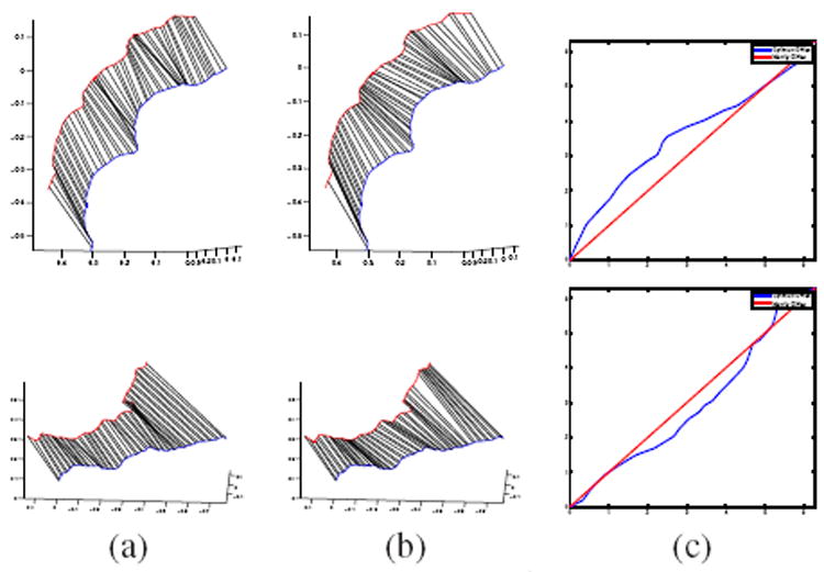
Each row shows an example of: (a) Curve registration obtained by a non-elastic geodesic using Eq. 4, (b) Curve registration obtained by an elastic geodesic using Eq. 5, and (c) optimal diffeomorphism γ̂ shown in blue, along with γ = s plotted in red.

3. Intrinsic Statistical Model for Sulci

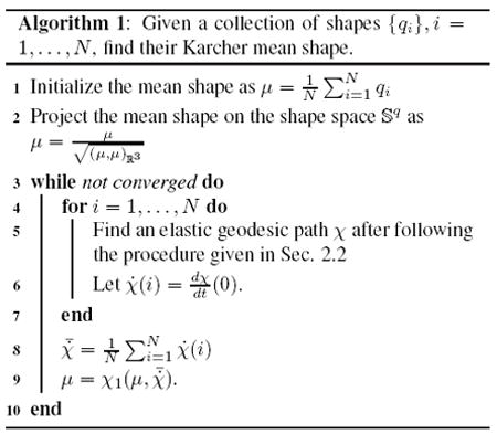
Having defined the framework for curve shape matching, we now construct a sulcal atlas of a large population of curves in the shape space. However, in order to do so, we need the notion of a shape average based on the sulcal and gyral curves. Owing to the nonlinearity of the shape space, the computation of an average shape is not straightforward. There are two well known approaches of computing statistical averages in such spaces. The extrinsic shape average is computed by projecting the elements of the shape space in the ambient linear space, where an Euclidean average is computed, and subsequently projected back to the shape space. On the other hand, the intrinsic average, also known as the Karcher mean ([1, 8]) is computed directly on the shape space, and makes use of distances and lengths that are defined strictly on the manifold. It uses the geodesics defined via the exponential map, and iteratively minimizes the average geodesic variance of the collection of shapes. The extrinsic average is simple and efficient to calculate, however it ignores the nonlinearity of the shape space, as well as depends upon the method used for embedding the manifold in the Euclidean space. As a simple example, a unit circle can be embedded inside ℝ² in several ways, and each embedding possibly leads to different values of extrinsicmeans on the circle. We will adopt the intrinsic approach by computing the Karcher mean for a given set of shapes. Algorithm 1 describes the procedure for computing the Karcher mean of a collection of shapes under the q representation.

Using Algorithm 1, we now construct a sulcal shape atlas for a population of 176 subjects. These subjects underwent high-resolution T1-weighted MRI scans with spatial resolution 1×1×1 mm³ on a Siemens 1.5T scanner. After preprocessing the raw data, and registering it stereotaxically to a standard atlas space, the cortical surfaces for these subjects were extracted using an automated algorithm [6]. For each of these subjects, a total of 28 landmark curves were manually traced. Figure 3 shows the original 28 landmark curves for each of the 176 subjects for the left hemisphere overlaid together. For the remainder of this paper, we will demonstrate the results on the left hemisphere of the brain to simplify things, although the same procedure can be repeated for the right hemisphere as well. Figure 3 also shows the intrinsic sulcal shape averages of the 28 landmark curves using Algorithm 1, as well as the respective extrinsic Euclidean averages for the same. While computing the extrinsic average, each curve for the same landmark type was mapped to its q representation, thus making it scale and translation invariant. The Euclidean average of all the q functions was then computed after a pairwise rotational alignment. Both the Karcher mean shapes as well as the Euclidean averages were then mapped back to the curve space in order to visualize them.

Figure 3.

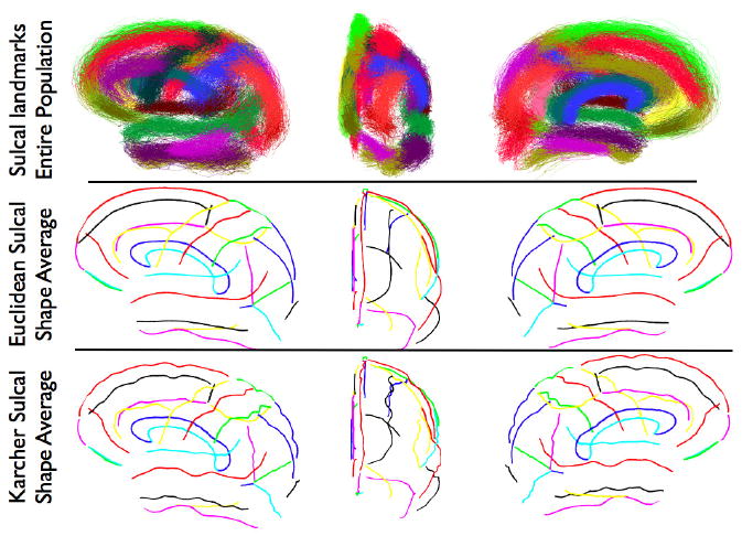
Lateral, frontal, and medial views of, Top row: 28 landmark sulci and gyri for 176 subjects, Middle row: Euclidean sulcal shape averages for each landmark, Bottom row: Karcher means for each landmark. (Best viewed in color).

It is observed that the intrinsic averages although smooth, have preserved important features along the landmarks, thus representing the average local shape geometry along the sulci and gyri. This also implies that the shape average has not only captured the salient geometric features, but has also reduced the shape variability in the population. In order to demonstrate this property, we plot the variance of the shape deformation for each landmark type as captured by the velocity vector along the geodesic path, both for Euclidean extrinsic, and Riemannian intrinsic averages. Thus for each of the 28 landmark average shapes for 176 subjects, μ̂_i, i = 1, … , 28, we plot the quantity $\frac{1}{176}{\sum }_1^{1}76\langle \dot{\chi }(i),\dot{\chi }(i)\rangle$, where χ(i) given in Algorithm 1, line 6. This quantity measures the invariant deformation between a pair of shapes, and only depends upon the intrinsic geometry of the shapes. Figure 4 shows a comparison of the plots of χ̇(i) for each of the landmarks, taken along the length of the curve, for both Euclidean shape averages, as well as intrinsic shape averages. This can also be thought of as the geodesic variance. From the color-coded map, it is observed that the intrinsic average has reduced the variance in terms of shape geometry deformation, and thus is a better representative of the population. This has important implications for surface registration as is demonstrated in the following section.

Figure 4.

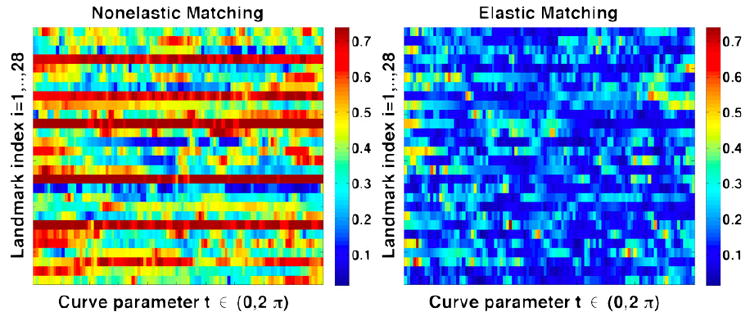
Comparison of the geodesic variance for the entire sulcal population for each of the 28 landmarks, both for Euclidean shape averages, as well as elastic shape averages, along the length of the curves.

4. Cortical Surface Registration using Landmark Curves

In this section, we briefly introduce our scheme for registering cortical surfaces. There have been prominent approaches [14, 7] for cortical registration in the neuroimaging community. The method, although based on the same conceptual framework of elastic registration, provides a slightly differentmodel for computing the deformation, and there are improvements in the implementation that increase flexibility and efficiency.

A general outline of the process is as follows. The first stage is to establish homology of the curve data, which is accomplished by matching the shapes in a Riemannian shape space framework. Next, the surfaces and curves are conformally mapped to the sphere, establishing a common space where deformation will be defined. Following this, there is a rotational alignment of the surfaces and curves to account for the differences in spherical mapping orientations. Next, the spherical mean of the curves is found to define the atlas curves for the domain of the deformation. Finally, the elastic deformation of the atlas on the sphere is found, which constrained to map the atlas curves to each case’s set of curves. The surfaces are reparameterized by this elastic deformation. The resulting surfaces then have homologous coordinate systems, allowing local comparisons across the group.

We define a set of N surfaces, {M₁, …,M_N} where M_i ⊂ ℝ³. We represent their mesh geometry using a set of simplicial complexes, {(K₁, f₁), …, (K_N, f_N)} where K_i is a simplicial complex and f_i : K ↦ M_i. For each surface i, we have a set of M landmarks represented by continuous open curves {β_i1, …, β_iM} where β_ij : [0, 2 π] ↦ M_i, and the set of curves {β_ij : i ∈ [1,N]} represent homologous regions on the set of surfaces. Additionally, the curves are discretized, where the j-th curve has k_j vertices.

4.1. Inverse Diffeomorphic Mapping of Landmark Curves

The first step of the process is to establish a correspondence between the homologous landmark curves by computing mappings γ̂_ij : [0, 2π] ↦ [0, 2π] such that for curve j and parameter t, {β_ij(γ_ij (t)) : i ∈ [1,N]} is a set of homologous points on the surfaces. This is accomplished by mapping the curves to a Riemannian manifold shape space, where reparameterizations are defined by geodesics to the Karcher mean of the curves in the shape space.

4.2. Spherical Mapping and Alignment

Next, the surfaces are mapped to the sphere, where the deformation will be computed. In general, a set of bijective mappings is found from each surface to the unit sphere, {ϕ₁, …, ϕ_N} where ϕ_i : M_i ↦ S². The spherical mapping of the matched curves is then $\stackrel{\sim }{{\beta }_{\mathit{ij}}}={\varphi }_1\circ {\beta }_{\mathit{ij}}\circ {\gamma }_{\mathit{ij}}$. The meshes are simplified using a QEM-based simplification and mapped to a sphere using a conformal mapping. The curves are then mapped to the sphere by using the barycentric coordinates of each curve vertex. A bounded interval hierarchy is used to efficiently search for the coincident face of each curve vertex. Once the meshes and curves are mapped to the sphere, they are rotationally aligned to enforce a consistent orientation of the spherical mappings. Given an arbitrarily chosen target, each set of curves is aligned to the target by computing the rotation and reflection that minimizes the least-squared difference between the discretized curve coordinates. This is accomplished by solving the unconstrained orthogonal Procrustes problem using singular value decomposition. Typically, left and right hemisphere surfaces will be available, and allowing reflections in the transform is advantageous in this case because both hemisphere can be mapped to a common orientation. So, for an arbitrary $T\in \{\stackrel{\sim }{{\beta }_{\mathit{ij}}}:i\in [1,N]\}$, we find an alignment R ∈ ℝ^3×3 as,

$$\begin{array}{lll}{R}_i& =& \arg \underset{\mathrm{\Omega }}{\min }\sum _j\sum _k\parallel \mathrm{\Omega }\left(\stackrel{\sim }{{\beta }_{\mathit{ij}}}\left(\frac{k-1}{k_j-1}\right)\right)-T\left(\frac{k-1}{k_j-1}\right)\parallel ,\\ & & \mathrm{where}{\mathrm{\Omega }}^T\mathrm{\Omega }=I\end{array}$$ (6)

We then optimally rotate the curves as well as the spherical maps as, ϕ̂_i = R_i ○ ϕ_i, and $\widehat{{\beta }_{\mathit{ij}}}=R_i\circ \widehat{{\beta }_{\mathit{ij}}}$.

4.3. Spherical Curve Atlas

Once the meshes and curves have been aligned on the sphere, the mean curves are computed. These mean curves will be used as the atlas curves in the surface warping. The Karcher mean on the sphere is found for each vertex of each curve, across the group. In this method, an initial guess is found by the normalized average of the points. For this point, the tangent space is defined by the gnomonic projection. A new mean is computed in the tangent space, and it is mapped back to the sphere and the process is repeated until the difference between the previous and the new mean is smaller than a threshold. We can express the curve atlas as the set $\{\overline{{\beta }_j}:j\in [1,M]\}$, where $\overline{{\beta }_j}$ is the karcher mean of $\{\widehat{{\beta }_{\mathit{ij}}}:i\in [1,N]\}$.

4.4. Elastic SurfaceWarping

For surface i, the deformation of the atlas is ϕ_i : S² ↦ S², where ${\varphi }_i(\overline{{\beta }_j}(t))=\widehat{{\beta }_{\mathit{ij}}}(t)$ for t ∈ [0, 2π], j ∈ [1, M]. Six bijective flattenings of the sphere are defined {φ_n : S² ↦ [0,1]² : n ∈ 1, 2, 3, 4, 5, 6}. For a point on the sphere, p ∈ S², the flattening is chosen as ${\phi }_p=\arg {\min }_{{\phi }_n}\parallel {\varphi }_n(p)-(\frac{1}{2},\frac{1}{2})\parallel$. The displacement field u_P : S₂ ↦ ℝ² is then u_p(x) = φ_p(ϕ_i(x)) − φ_p (x). At non-landmark points, i.e. $x\in S^2,x\notin {\cup }_j\{\widehat{{\beta }_{\mathit{ij}}}(t):t\in [0,2\pi ]\}$, the mapping is constrained to satisfy a small deformation nonlinear elastic model similar to Thompson et al. [14], and is given by

$$\mu {\nabla }^2{u}_p(x)+(\lambda +\mu )\nabla (\nabla \cdot u_p(x))=0$$ (7)

Computationally, the atlas mesh is defined on the sphere by tessellating the sphere with a subdivided octahedron, shown in Figure 5 [11]. This representation is advantageous for its multiscale and flattened representation. Sub-division of each triangle is performed by adding vertices at the midpoints of the edges, then adding new edges connecting them, creating four triangles from the original. This scheme is used for defining the representations of the mesh in multiscale algorithms. Furthermore, this subdivision process ensures that the mesh can be flattened to a rectangular and regularly sampled grid. This flattening can be imagined as follows. First, choose one of the vertices of the octahedron, this will be mapped to the center of the grid. Then cut the four far edges that do not contain the center vertex. These edges are duplicated and define the boundary of the grid, and the opposite vertex maps to the four corners of the grid. This is illustrated in Figure 6. This flattened representation allows for efficient interpolation, smoothing and finite differences operations on the grid [11].

Figure 5.

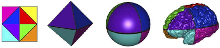
Mappings between the grid, octahedron, sphere and a cortical surface

Figure 6.

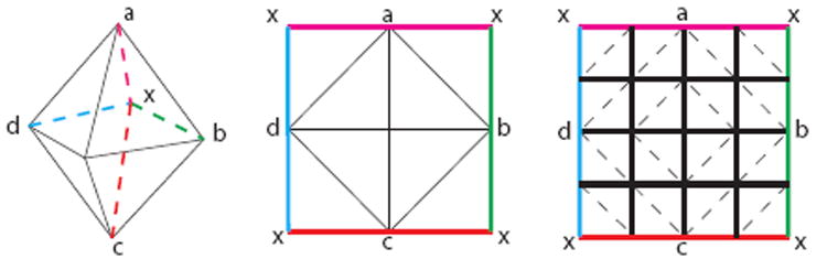
The flattening and an example of two subdivisions.

The deformation is computed iteratively using finite differences with a multigrid method. The octahedral domain is particularly suitable for this because the representation lends to simple prolongation, restriction and smoothing multigrid operations. The solver accounts for the spherical topology of the domain by solving the equation in the flattening of the mesh at the vertex that is being updated, mapping neighboring vertex values relative to this flattening, as described above. Each mesh is resampled by the deformed atlas, establishing vertex homology between the meshes.

5. Results

In this section, we demonstrate results of cortical surface registration with and without the incorporation of the elastic sulcal shape analysis. The data consists of cortical surfaces of 176 subjects collected and processed according to the procedure described in Section 3. The sulcal shape atlas is already constructed and shown in Fig. 3. We now compute geodesics between the average shape of the landmark, and the set of all sulci belonging to that landmark type, and reparameterize the set of sulci according to inverses of the resulting diffeomorphisms. We then follow the steps outlined in Sec. 4 in order to warp all the surfaces meshes to the atlas. Figure 7 shows the flattened representation of a surface atlas colored according to curvature of the surface. The figure shows flattened atlases for surfaces without any landmark curves, surfaces with landmark curves using Euclidean analysis, and finally surfaces with landmark curves using the diffeomorphic shape analysis. In the absence of landmark curves, the atlas shows smoothing of corresponding features and information present in the population, while in the presence of landmarks, the general landmark features reappear in the atlas. However the most interesting case is shown in Fig. 7 (c), where not only do the landmark curves manifest themselves as before, but they also exhibit rich local geometry that has been preserved due to the elastic diffeomorphisms. Additionally, Fig. 8 shows three the lateral, dorsal, and medial views of the reconstructed cortical surface from the flattened representations. It is observed that the surface with diffeomorphic shape analysis shows richer geometric detail than the typical Euclidean analysis.

Figure 7.

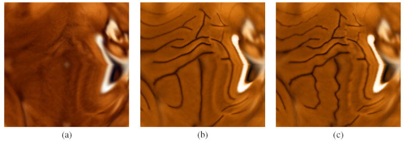
Average flattened representations for atlases: (a) without landmark curves, (b) with landmark curves using Euclidean analysis, (c) with landmark curves using the diffeomorphic shape analysis.

Figure 8.

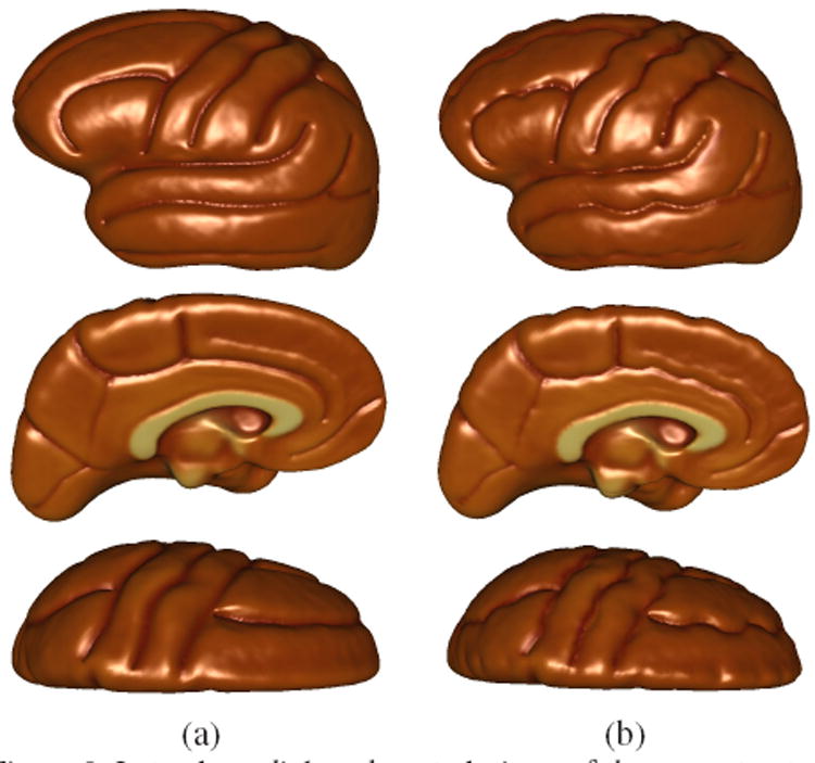
Lateral, medial, and ventral views of the reconstructed cortical surface with (a) Euclidean landmark analysis, and (b) diffeomorphic shape analysis.

6. Conclusion

We have presented a geometric method for shape analysis of sulcal and gyral features and demonstrated their use in cortical surface registration. Although, the method models shape averages of cortical sulci and gyri, the theory itself is quite general and is applicable to diverse surface correspondence problems that use landmarks to guide the warping. Thus surface registration accuracy is improved, not only by the inclusion of increasing number of landmarks, but largely by the proposed intrinsic, elastic shape analysis framework.

References

- 1.Bhattacharya R, Patrangenaru V. Nonparametic estimation of location and dispersion on Riemannian manifolds. Journal of Statistical Planning and Inference. 2002 Jan;108(1-2):23–35. [Google Scholar]
- 2.Dale AM, Fischl B, Sereno MI. Cortical surface-based analysis. I. segmentation and surface reconstruction. NeuroImage. 1999 Feb;9(2):179–94. doi: 10.1006/nimg.1998.0395. [DOI] [PubMed] [Google Scholar]
- 3.Duchesnay E, Cachia A, Roche A, Riviere D, Cointepas Y, Papadopoulos-Orfanos D, Zilbovicius M, Martinot J-L, Regis J, Mangin J-F. Classification based on cortical folding patterns. IEEE Tran Med Imaging. 2007 Jan;26(4):553–565. doi: 10.1109/TMI.2007.892501. [DOI] [PubMed] [Google Scholar]
- 4.Fischl B, Rajendran N, Busa E, Augustinack J, Hinds O, Yeo BTT, Mohlberg H, Amunts K, Zilles K. Cortical folding patterns and predicting cytoarchitecture. Cereb Cortex. 2008 Aug;18(8):1973–80. doi: 10.1093/cercor/bhm225. [DOI] [PMC free article] [PubMed] [Google Scholar]
- 5.Fischl B, Sereno MI, Dale AM. Cortical surface-based analysis. II: Inflation, flattening, and a surface-based coordinate system. NeuroImage. 1999 Feb;9(2):195–207. doi: 10.1006/nimg.1998.0396. [DOI] [PubMed] [Google Scholar]
- 6.Holmes C, MacDonald D, Sled J, Toga A, Evans A. Cortical peeling: CSF/grey/white matter boundaries visualized by nesting isosurfaces. Lecture notes in computer science. 1996 Jan;1131:99–104. [Google Scholar]
- 7.Joshi A, Shattuck D, Thompson P, Leahy R. Surface-constrained volumetric brain registration using harmonic mappings. IEEE Tran Med Imagng. 2007 Dec;26(12):1657–1669. doi: 10.1109/tmi.2007.901432. [DOI] [PMC free article] [PubMed] [Google Scholar]
- 8.Le H. Locating Fréchet means with application to shape spaces. Advances in Applied Probability. 2001 Jan;33(2):324–338. [Google Scholar]
- 9.Leow A, Yu C, Lee S, Huang S, P H. Brain structural mapping using a novel hybrid implicit/explicit framework based on the level method. NeuroImage. 2005 Jan;24:910–927. doi: 10.1016/j.neuroimage.2004.09.022. [DOI] [PubMed] [Google Scholar]
- 10.Lohmann G, von Cramon DY, Colchester ACF. Deep sulcal landmarks provide an organizing framework for human cortical folding. Cereb Cortex. 2008 Jan;18(6):1415–1420. doi: 10.1093/cercor/bhm174. [DOI] [PubMed] [Google Scholar]
- 11.Losasso F, Hoppe H, Schaefer S, Warren J. Smooth geometry images. ACM SIGGRAPH Symposium on Geometry processing. 2003 Jan;43:138–145. [Google Scholar]
- 12.Mangin J, Riviere D, Cachia A, Duchesnay E, Cointepas Y, Papadopoulos-Orfanos D, Scifo P, Ochiai T, Brunelle F, Regis J. A framework to study the cortical folding patterns. NeuroImage. 2004 Jan;23:S129–S138. doi: 10.1016/j.neuroimage.2004.07.019. [DOI] [PubMed] [Google Scholar]
- 13.Tao X, Han X, Rettmann M, Prince J. Statistical study on cortical sulci of human brains. Lecture notes in computer science. 2001 Jan;:475–487. [Google Scholar]
- 14.Thompson P, Toga A. A surface-based technique for warping 3-dimensional images of the brain. IEEE Tran Med Imagng. 1996 Jan;15(4):402–417. doi: 10.1109/42.511745. [DOI] [PubMed] [Google Scholar]
- 15.Vaillant M, Davatzikos C. Finding parametric representations of the cortical sulci using an active contour model. Medical Image Analysis. 1997 Jan;1(4):295–315. doi: 10.1016/s1361-8415(97)85003-7. [DOI] [PubMed] [Google Scholar]