Noninvasive Temperature Mapping With MRI Using Chemical Shift Water-Fat Separation

Abstract

Tissues containing both water and lipids, e.g., breast, confound standard MR proton reference frequency-shift methods for mapping temperatures due to the lack of temperature-induced frequency shift in lipid protons. Generalized Dixon chemical shift–based water-fat separation methods, such as GE’s iterative decomposition of water and fat with echo asymmetry and least-squares estimation method, can result in complex water and fat images. Once separated, the phase change over time of the water signal can be used to map temperature. Phase change of the lipid signal can be used to correct for non-temperature-dependent phase changes, such as amplitude of static field drift. In this work, an image acquisition and postprocessing method, called water and fat thermal MRI, is demonstrated in phantoms containing 30:70, 50:50, and 70:30 water-to-fat by volume. Noninvasive heating was applied in an Off1-On-Off2 pattern over 50 min, using a miniannular phased radiofrequency array. Temperature changes were referenced to the first image acquisition. Four fiber optic temperature probes were placed inside the phantoms for temperature comparison. Region of interest (ROI) temperature values colocated with the probes showed excellent agreement (global mean ± standard deviation: −0.09 ± 0.34°C) despite significant amplitude of static field drift during the experiments.

Hyperthermia shows great promise both as a primary or an adjunct treatment for a variety of malignancies. In addition, high-frequency focused ultrasound has been demonstrated to be effective for treating superficial and deep tumors in soft tissue (1,2). Conventional, lower-temperature hyperthermia therapies have been shown to be effective as an adjunct treatment (3) with radiation or chemotherapy in such cases as recurrent tumors in the chest wall (4) and sarcomas in leg and other extremities.

Accurate tumor and normal tissue temperature measurements are necessary to confirm desired thermal dose distributions, a key factor for successful treatment (3,5,6). Invasive thermometry provides accurate but spatially limited measurements. Devices such as fiber optic probes are often limited to a single location or a one-dimensional track through the region of interest, due both to accessibility and patient tolerance. Regional temperature mapping via MR methods should increase control of the therapy distribution by providing a three-dimensional distribution of temperatures, using a noninvasive technique (7).

Previous work has shown the value of using the temperature sensitivity of the tissue water proton resonant frequency shift (PRFS) (8-11). The temperature dependency of water protons is approximately 0.01 PPM/°C (12), which in a 1.5-T scanner results in 0.64 Hz/°C. This effect can be observed in its most simple form via a gradient echo data acquisition, where a series of images of a water-based gel phantom is acquired through time while applying heat. If each complex image is subtracted from the first and the phase angle for each time point plotted against time, then the phase change over time directly correlates to the change in temperature. However, tissues with a mix of water and lipids, e.g., breast, confound most standard PRFS approaches because lipids have no chemical shift dependence with temperature (13).

The separation of water and fat signals into separate images is an active and growing area of research, with numerous clinical and clinical research applications (14-20). Most techniques developed differentiate these signals by exploiting the chemical shift differences between water and fat signals (~210 Hz between water and the methylene resonance at 1.5 T). Both two-point and multipoint sequences exist, and both types have been shown to be sensitive to the effects of T₂* bias, T₁ bias, and the accuracy of the spectral modeling for fat resonances (21,22). Mixed water and fat within a voxel has also been used by one group to correct PRFS measurements for field changes during MR thermometry imaging (23).

In this paper, we demonstrate an image acquisition and postprocessing method for thermal imaging in tissues containing both water and fat, called water and fat thermal (WAFT) MRI. For this work, we made use of an offline implementation of the IDEAL (iterative decomposition of water and fat with echo asymmetry and least-squares estimation) (18-20,24) water-fat separated imaging algorithm; however, theoretically any technique that results in separate complex images of water and fat could have been used. The IDEAL method is a multiecho algorithm that allows data acquisition echo times (TE) to be generalized. Extensions in the original IDEAL method have been developed to account for T₂* and T₁ bias artifacts and to allow a multispectral peak model to be used to improve fat fraction estimates. The algorithm also accounts for amplitude of static field (B₀) inhomogeneities across a sample. The complex signal phase changes between the water and fate images due to heating over time are exploited to determine tissue temperature change while avoiding apparent variations in temperature measurements due to global B₀ changes.

MATERIALS AND METHODS

WAFT-MRI Theory

In its most commonly used form, the IDEAL technique uses complex MR image data acquired at three or more TE to estimate the complex water and fat contributions and B₀ inhomogeneity in each voxel. The complex water and fat signals in a voxel can be modeled by:

$$S\left(t_n\right)=\left(A_w\exp \left(i{\mathrm{\varphi }}_w\right)+A_f\exp \left(i{\mathrm{\varphi }}_f\right)\exp \left({\mathit{if}}_{\mathit{cs}}{t}_n\right)\right)\exp \left(i\mathrm{\Psi }{t}_n\right)$$ [1]

where A_w exp(iϕ_w) and A_f exp(iϕ_f) represent the complex signals from water and fat protons, respectively. The frequency difference due to chemical shift between water and fat is accounted for by the term exp(if_cst_n). Global frequency changes (e.g., B₀ drift) are accounted for by the Ψt_n term. A minimum of three TE is required to solve for the five independent variables, A_w, A_f, ϕ_w, ϕ_f, and Ψ. Note that the estimated water and fat signals are complex, with independent phase.

Due to chemical shift, aka shielding interactions, water protons display a marked frequency shift with temperature change, while protons attached to fat do not. As the water frequency changes with temperature, this adds a frequency shift over time in the water term. When the water signal in IDEAL processing is modeled as being on-resonance, temperature changes result in an apparent phase change in the fat term:

$$S\left(t_n\right)=\left(A_w\exp \left(i{\mathrm{\varphi }}_w\right)+A_f\exp \left(i{\mathrm{\varphi }}_f\right)\exp \left(i{\mathrm{\varphi }}_{\mathit{cs}}{t}_n\right)\times \exp \left(-i{\mathrm{\varphi }}_{\mathrm{\Delta }{T}_n}\right)\right)\exp \left(i\mathrm{\Psi }{t}_n\right)$$ [2]

The apparent phase change in the fat signal is ϕ_ΔTn = ω_ΔTt_n, where ω_ΔT is the frequency shift in radians due to temperature change. This apparent temperature-dependent phase change in fat can be solved for by calculating voxel by voxel the fat signal phase angle difference between each reconstructed fat image. However, we found that the calculation of the phase angle difference between the water and fat signals was more useful. This value references changes due to temperature to the fat signal in the voxel, which is inherently insensitive to temperature but accounts for phase changes due to all other mechanisms, such as B₀ drift.

The temperature dependency of water protons is approximately 0.01 PPM/°C (12), which in a 1.5 T scanner results in 0.64 Hz/°C. The effect of this relatively small frequency shift can be amplified in gradient echo pulse sequence data by using longer TE to acquire data, e.g., a TE = 4 ms yields 0.92° of phase per degree Celsius; however, a TE = 20 ms gives approximately 4.6° of phase per degree Celsius.

The complex fat signal is actually composed of multiple spectral lines at different chemical shift offsets due to the variability of the magnetic microenvironment experienced by protons in the lipid chain. The phase of each fat resonance thus changes differently with time. A number of groups have shown that the accuracy of water-fat-separated image methods improve when the fat signal model accounts for this spectral distribution (14,22). This is particularly important when acquiring data at longer TE values as the phase differential between lipid groups is further exaggerated. Thus, we can write the complex fat signal with N lines, relative amplitudes p_n, and relative signal phases of ϕ_fn as:

$$A_f\exp \left(i{\mathrm{\varphi }}_f\right)=A_f{\displaystyle \sum _{n=1}^N{p}_n\exp (i\mathrm{\Delta }{\mathrm{\varphi }}_{f_n})\mathrm{where}}{\displaystyle \sum _{n=1}^N{p}_n=1}.$$ [3]

Phantom Data and WAFT-MRI Postprocessing

Three water-fat phantoms consisting of peanut-oil-in-gelatin dispersions (25) were created. The phantoms’ water-to-fat ratios were 30:70, 50:50, and 70:30 by volume. The water-fat solution of each phantom was doped with salt to approximately physiologic saline levels to improve coupling for radiofrequency (RF) heating. The melting point of the gelatin matrix occurs at over 100°C. The 50:50 and 70:30 phantoms were built in 5 × 10 inch (diameter × length) cylindrical plastic tubes, but the 30:70 phantom was built in a 4.25 × 7 inch cylindrical plastic tube to simplify the creation of this phantom and improve the homogeneity of the water and fat ratio throughout. Four catheters were inserted along the length of each phantom, one at the center of each cylinder and three near the outside edge of the phantom at 120° offsets from each other. The catheters allowed the insertion of invasive Lumasense fluorescent probes (Lumasense Technologies, Santa Clara, CA) to measure actual temperatures at MR image locations during image acquisitions.

Single-voxel, short-TE MR point-resolved spectroscopy was used to determine fat peak frequency values and relative amplitude ratios. Acquisition parameters were pulse repetition time = 5 sec, TE = 30 ms, SW = 2000 Hz, 2048 points, and eight averages with no water suppression. Single-voxel, short-TE MR point-resolved spectroscopy voxels were acquired from 1-cm³ voxels centered at each of the catheter locations midway along the length of each phantom to determine the homogeneity of each solution (Fig. 1). The SITools-FITT software package (26) was used to fit areas and frequencies beneath a single water peak and six lipid peaks (Fig. 2).

FIG. 1.

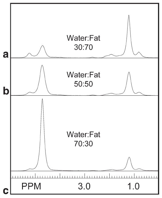
Single-voxel MR spectra (single-voxel, short-TE MR point-resolved spectroscopy; TE = 30 ms) of 1-cm³ voxels from the three water-fat phantoms. Phantoms were composed of peanut oil in gelatin dispersions at (a) water-fat 30:70, (b) water-fat 50:50, and (c) water-fat 70:30 ratios by volume. Water consists of a single peak at 4.7 PPM; all other peaks are due to lipid resonances.

FIG. 2.

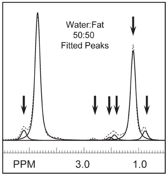
Fitted peaks for peanut oil resonances and water. This spectrum was acquired from the 50:50 water-to-fat-ratio phantom. Six resonances were sufficient to characterize the lipid peaks, as indicated by the arrows at 5.22, 2.69, 1.96, 1.21, and 0.78 PPM.

Each phantom was actively heated, independent of the other two, in a miniannular phased array (MAPA) (27) with four RF antennas. A water bolus sleeve (see Fig. 3a) was used to improve coupling of the RF energy at 140 MHz into the water-fat phantom. D₂O (99.8% pure; Sigma Aldrich #617385, St. Louis, MO) was used to fill the bolus sleeve to minimize image artifacts from convection currents. Four narrow, cylindrical references containing only silicone oil were located both inside the water bolus and along the sides of the MAPA. These references provide pure fat signals for B₀ drift corrections during PRFS measurements but were not necessary for this experiment. Each water-fat phantom was positioned in the center of the MAPA and RF heating was applied in an Off1-On-Off2 pattern. During the On period, all four RF antennae were set to 15 W continuous power to heat the phantom with a symmetric distribution. Lumasense temperature probes were centered within the MR slice and recorded temperatures every 10 sec for the duration of the experiment. A text file record of Lumasense measurements was saved offline for comparison to reconstructed temperature maps.

FIG. 3.

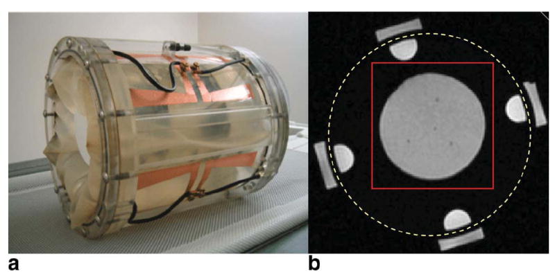
a: MAPA RF heating device. b: Axial magnitude gradient echo image with TE = 16.1 ms of 50:50 water-fat phantom (inner gray circle) surrounded by a D₂O-filled bolus (black) with fat-filled half-cylinder internal and rectangular outer references. The dotted yellow circle indicates outer diameter of the MAPA former. The red square indicates the region of the acquired images that was postprocessed for temperature maps, as displayed in subsequent figures. [Color figure can be viewed in the online issue, which is available at www.interscience.wiley.com.]

Complex MR image data were acquired on a GE Signa HDX 1.5T system (GE Healthcare, Waukesha, WI). Five gradient echo images were taken at each time point. A single slice was positioned at the center of the MAPA/phantom, with 6mm slice thickness, TE = [16.78, 19.84, 22.91, 25.98, 29.04 ms], pulse repetition time = 34 ms, field of view = 30 cm, 128 × 128 points, receive band width 32 kHz, and averages = 2. Nominal voxel size was 2.4 × 2.4 × 6mm. Five TE were acquired to permit the temperature map algorithm to determine if a five-echo fit permitted a better estimate than a three-echo fit. Total data acquisition for the five echoes was approximately 2 min. Over 52 min, 25 time points were acquired, with approximately 20 min heat Off1, 20 min with heat On (15 W × four channels), and 12 min heat Off2. Complex image data were transferred offline and temperature maps reconstructed using in-house software written in IDL (ITT-VIS, Boulder, CO).

Standard IDEAL image reconstruction, without T₂* correction, yielded complex image estimates for water and fat, using both three- and five-echo reconstruction algorithms. Heating resulted in the addition of an apparent complex phase component to the fat image. In each voxel, the phase accumulation due to temperature was calculated by taking the difference between the current water-fat phase angle, atan(ϕ_w − ϕ_f), and the water-fat phase angle for the previous image acquired. The total phase change due to heating was calculated as the sum of the changes at each time point. Based on the assumption that the phase change due to temperature ϕ_ΔTn = ω_ΔT t_n was small between the N echoes acquired for the IDEAL reconstruction, the temperature change was be calculated via ϕ_ΔT ~ ω_ΔT TE_N/2, where TE_N/2 was the middle TE value collected for IDEAL reconstruction. Each IDEAL image reconstruction was performed independent of all other time points. The above assumptions were made based on an expectation for smoothly distributed temperature changes. Because image noise from each data collection can lead to small variations in IDEAL image reconstruction, we expect variations in temperature measurements to also be independent of time points and related to image noise.

RESULTS

An example of water-fat phantom single-voxel, short-TE MR point-resolved spectroscopy spectra is shown in Fig. 1 from center voxels positioned in the (Fig. 1a) 30:70, (Fig. 1b) 50:50, and (Fig. 1c) 70:30 phantoms. An example of fitting the center spectrum from the 50:50 water-fat phantom is shown in Fig. 2. A total of 12 spectra were fitted across three phantoms. Six spectral lines were used to characterize the fat, as indicated by the arrows in Fig. 2. Due to their similarity, fat peaks 3 and 4 were combined to simplify the IDEAL calculation. Fat peak areas were normalized to the total fat area. The mean PPM and area of each peak were used in the IDEAL reconstruction; these were 5.22, 2.69, 1.96, 1.21, and 0.78 PPM and 0.071, 0.012, 0.091, 0.734, and 0.092 for the respective areas. Standard deviations for fitted values in the 50:50 phantom were on the order of 2-8%, except for the smallest peak, at 2.69 PPM with a 20% standard deviation.

Figure 3 shows (Fig. 3a) the MAPA RF heating device and (Fig. 3b) a representative axial gradient echo image for TE = 16.1 ms, with the water-fat phantom (gray, center) supported by the D₂O bolus sleeve (dark) with fat-filled outer oil references (gray). The dotted yellow circle indicates outer diameter of the MAPA former. The red square indicates the region of the acquired images that was postprocessed for temperature maps. Signal-to-noise ratio for all water-fat phantoms ranged between 12 and 100:1, depending on water-fat ratio and in/out phase characteristics due to TE. Figure 4 shows the results for IDEAL reconstructed (Fig. 4a,c) water-only images and (Fig. 4b,d) fat-only images for the 50:50 phantom. Figure 4a,b was constructed from data with no heating applied. Figure 4c,d was constructed from data taken at maximum temperature change at time equal approximately 42 min. Similarly homogeneous water-fat images were reconstructed for all phantoms, although, as in Fig. 4c, some slight shading was seen in the water images in areas with the highest temperature changes due to T₁ changes due to temperature.

FIG. 4.

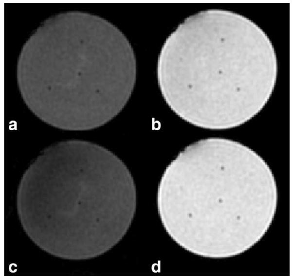
IDEAL reconstructed (a,c) water-only images and (b,d) fat-only images for phantom with 50:50 water-to-fat ratio. Images (a,b) were constructed from data with no heating applied. Images (c,d) were constructed from data taken at maximum temperature change, time ~42 min. Catheters for the four Lumasense fiber optic temperature probes can be seen as four small signal-hypo-intense areas in the center and around the edge of each phantom.

B₀ maps reconstructed from the IDEAL algorithm are shown in Fig. 5 for both the three- and five-echo reconstructions of the 50:50 phantom at the first time point. Both maps (Fig. 5a,b) show spatially inhomogeneous fields with a range of approximately 20 Hz across the phantom. B₀ values at the locations of the four Lumasense probes are shown in Fig. 5c,d for all time points of the experiment. These plots show that the spatially inhomogeneous pattern persists throughout the experiment but also displays a global drift with time.

FIG. 5.

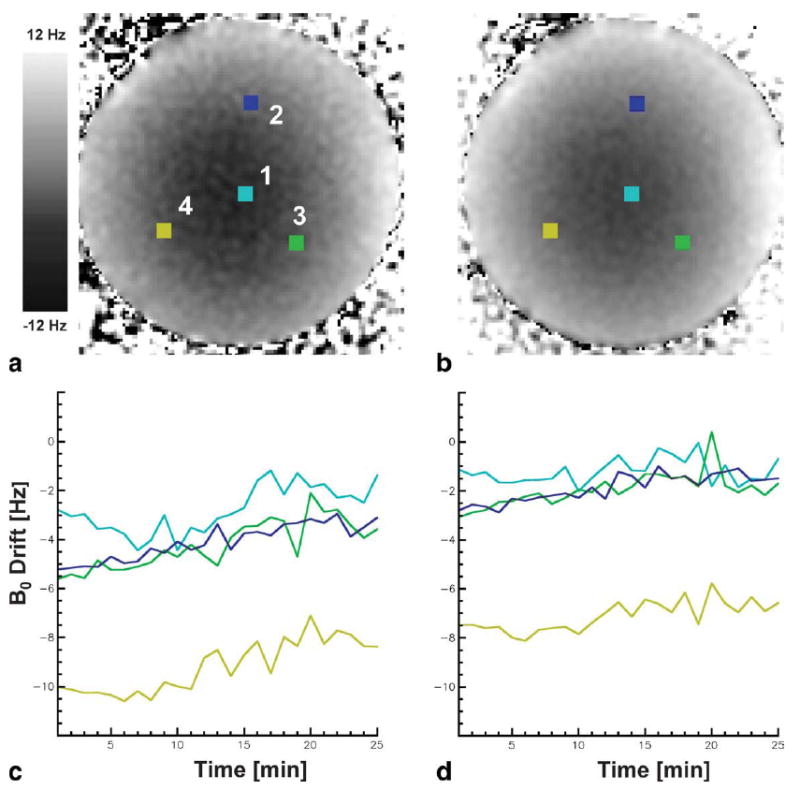
IDEAL calculated B₀ maps using (a) three and (b) five echoes in the 50:50 water-fat phantom. The four colored squares marked 1, 2, 3, and 4 show the placement of the 5 × 5 pixel ROIs that overlie the location of the Lumasense fiber optic temperature probes. Plots (c,d) show the B₀ drift for all time points for the four ROIs marked. A spatially inhomogeneous field with a global range of approximately 20 Hz is shown. This pattern persisted through time but showed a global field drift.

WAFT-MRI calculated temperatures are compared to Lumasense temperature measurements in 12 plots in Fig. 6. Each of the four Lumasense locations in a given phantom is shown vertically, while the same Lumasense in each of the three phantoms is shown horizontally. The mean of the first 20 Lumasense temperatures has been subtracted from each overall Lumasense plot to enable the relative changes of the WAFT-MRI values to be compared to the absolute Lumasense measurements. The Lumasense values show a flat baseline temperature change near 0°C during the initial period without heating (Off1) and a smooth increase in temperature during heating (On). Maximum temperature change varied between 4 and 9°C, depending on probe location. WAFT-MRI plots show excellent agreement with the Lumasense values for all locations and phantoms. Table 1 shows the variability in WAFT-MRI calculation about 0°C after subtracting the “gold standard” Lumasense values. For the initial nine time points, corresponding to the no-heat-applied period, the temperature variability was −0.11 ± 0.20°C for the three-echo reconstruction and −0.06 ± 0.17°C for the five-echo reconstruction. For the all 25 time points, the temperature variability was −0.21 ± 0.34°C for the three-echo reconstruction and −0.03 ± 0.29°C for the five-echo reconstruction. Further breakdown by phantom ratios and grouped values is also shown.

FIG. 6.

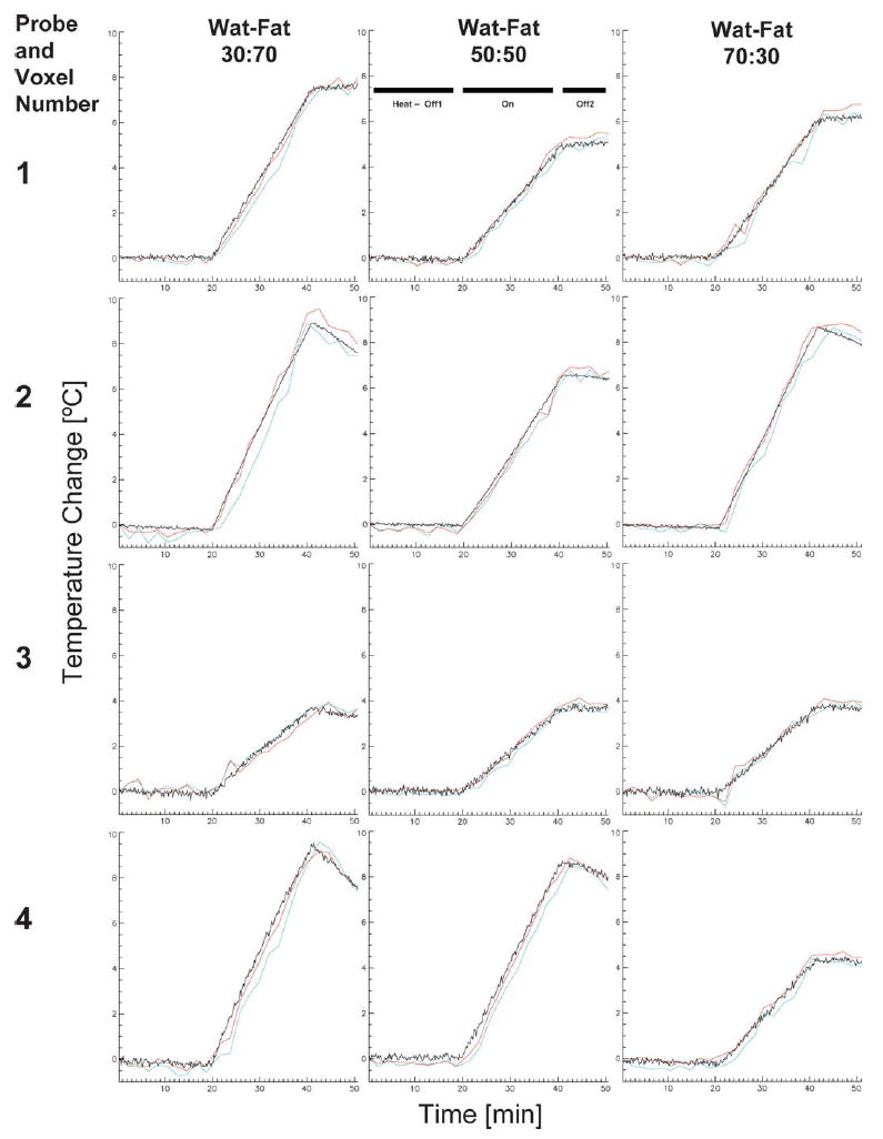
Temperature values from the ROIs indicated in Fig. 5a that overlie the four Lumasense fiber optic temperature-probe locations. WAFT-MRI values calculated with three echoes are plotted in blue; values calculated with five echoes are shown in red. Lumasense values are plotted in black. RF heating (On) started at approximately 20 min into the experiment and was turned off at 40 min (Off2). Rows show the value for a given Lumasense location in the 30:70, 50:50, and 70:30 water-fat ratio phantoms, respectively. Columns show the results for the four Lumasense locations—1, center; 2, top; 3, bottom right; and 4, bottom left—in a given phantom. WAFT-MRI measurements showed good agreement for most locations and slightly better agreement with the Lumasense values for three echo calculations than for five echo calculations.

Table 1.

Temperature Variation of WAFT-MRI Values Minus Lumasense Values for Three-Echo and Five-Echo Reconstructions^*

	WAFT-MRI minus Lumasense three-echo reconstruct (°C) (mean ± SD)	WAFT-MRI minus Lumasense five-echo reconstruct (°C) (mean ± SD)	WAFT-MRI minus Lumasense both reconstruct (°C) (mean ± SD)
Time points 2–18 min (heat Off1)
Water-fat 30:70	−0.151 ± 0.246	−0.043 ± 0.185	−0.097 ± 0.225
Water-fat 50:50	−0.100 ± 0.135	−0.079 ± 0.165	−0.090 ± 0.150
Water-fat 70:30	−0.088 ± 0.202	−0.044 ± 0.175	−0.066 ± 0.189
All phantoms	−0.113 ± 0.199	−0.055 ± 0.174	−0.084 ± 0.189
Time points 2–52 min (heat Off1-On-Off2)
Water-fat 30:70	−0.337 ± 0.428	−0.014 ± 0.298	−0.175 ± 0.402
Water-fat 50:50	−0.153 ± 0.266	−0.029 ± 0.269	−0.062 ± 0.282
Water-fat 70:30	−0.133 ± 0.279	0.071 ± 0.288	−0.031 ± 0.300
All phantoms	−0.208 ± 0.344	0.029 ± 0.286	−0.090 ± 0.337

^*Values are grouped for both reconstructions and broken down for individual and grouped phantoms. Results are further broken down for variations around the first nine time points, when there was no heating applied, and then for all time points. SD, standard deviation.

WAFT-MRI temperature maps are shown in Fig. 7 for all three phantoms at six time points, two in the initial no heat period (Off1), three in the heating period (On), and a final one in the second no-heat period (Off2). Temperature maps show a smooth transition of values both spatially and temporally for all phantoms. Despite equal power on all MAPA RF elements, the maps show asymmetric heat patterns. However, the same pattern is seen on all phantoms, indicating that the asymmetry was likely due to a slight systemic miscalibration of the MAPA RF amplifiers.

FIG. 7.

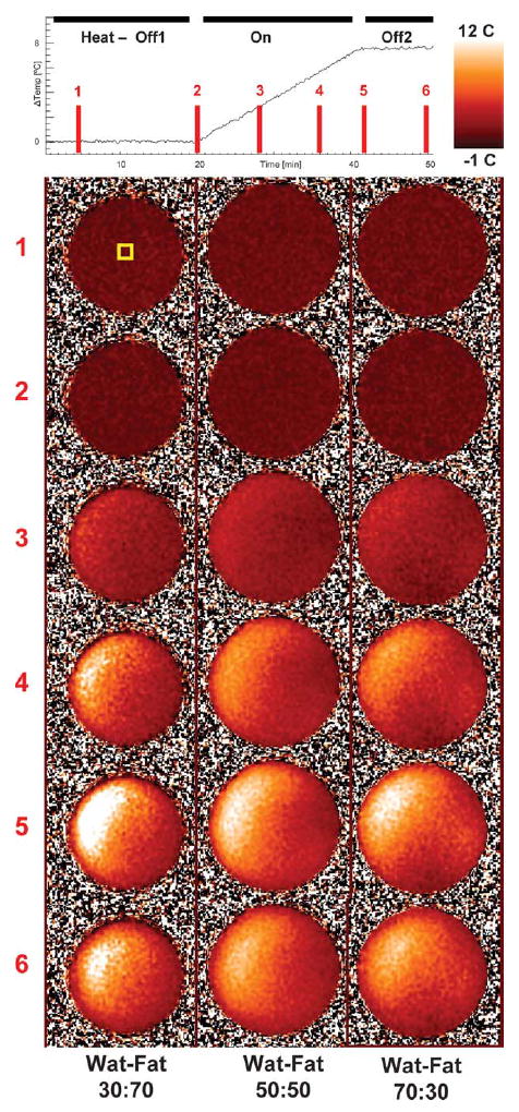
WAFT-MRI temperature maps for all water-fat phantoms at six time points during data acquisition. The yellow ROI indicated in the Time 1 map shows the location of the Lumasense probe, whose values are plotted at the top. RF heating was set equally for all antennas at all time points during the On period from minute 20 till minute 40 to ensure smooth heating.

DISCUSSION

Both visual inspection and the temperature variations in Table 1 demonstrate that the WAFT-MRI method agrees very well with Lumasense measurements. The mean temperature values for both the initial period without heat (Off1) and the entire time course were within 1 standard deviation of 0°C in all phantoms, regardless of the reconstruction method. Mean temperatures for both the three-echo and five-echo reconstruction methods remained consistent throughout the data collection, but the standard deviations for the entire heating period (Off1-On-Off2) were almost double those for the initial (Off1) period alone.

As there was no heating in the Off1 period, we would not expect the assumptions made for the WAFT-MRI method to interfere with the IDEAL reconstruction. These temperature variations are likely the most representative of the error due to image noise and the water-fat estimation assumptions made by the IDEAL method and thus a limit of the WAFT-MRI method. Work has been done to determine optimized TE values for improving the accuracy of the water-fat IDEAL estimates; however, such optimization was beyond the scope of this work. The TE values chosen for this report were ones empirically shown to produce reasonable results.

A significant benefit of the WAFT-MRI method over the PRFS method is that it provides inherent independence from artifacts due to B₀ drift. The WAFT-MRI method calculates temperature changes using the phase angle between water and fat. This allows the apparent phase change in the fat to be self-referenced in the same voxel to the fixed frequency water signal. Because both signals are affected equally by the B₀ drift and corrected equally by the IDEAL reconstruction estimate of B₀ changes both spatially and with drift over the 50-min heating period (approximately ±40 Hz spatially and ±5 Hz/h in this experiment), the method was not susceptible to artifacts due to B₀ inhomogeneity, as is the PRFS method. However, if significant B₀ changes occur within the total acquisition time of all echoes for an image, such as can occur in a breast during normal breathing (28), this could result in artifacts in both the water-fat and temperature images. One possible solution will be to use a high-speed multiecho acquisition to acquire data during a single breath hold.

Temperature results in this report were similar for all phantoms, regardless of water-fat ratio; however, the WAFT-MRI method is expected to fail as the voxel fat-water ratio approaches 0% or 100%. In organs containing compartments with both water and fat or just water, the data collected for IDEAL water-fat image reconstruction could also be used to perform a PRFS temperature change analysis. With the B₀ estimates created during the WAFT-MRI measurements, the B₀ drift found in water and fat compartments could also be used to estimate field drift corrections for the water-only compartments, using a PRFS measure. In both cases, it could be possible for the phase accumulated due to temperature change to exceed 360° and require phase unwrapping to differentiate actual changes. However, TE times can be selected for the WAFT-MRI method that can accommodate the range of temperatures expected to within one phase cycle. Also, by accumulating the change in phase between each temperature time point, rather than by comparison with an initial baseline value, phase unwrapping is not needed in a normal PRFS calculation either.

A drawback to the data collection method in this report was that we were unable to acquire our data using a multiecho sequence on our MR system, although multiecho implementations of IDEAL have been described (22,29). Individual echoes were acquired sequentially and overall acquisition time was approximately 2 min for five echoes. This imposed some necessary limitations to our spatial and temporal coverage. We acquired two averages to ensure sufficient signal-to-noise ratio to test our method. Based on the signal-to-noise ratio of our data and because the IDEAL water-fat images are reconstructed from three images, averaging was not necessary. Also, we were only able to acquire one slice in a reasonable amount of time. A multiecho sequence would have facilitated improved coverage. On higher field scanners, say at 3 T, where the chemical shift of water-fat is twice that at 1.5 T, it may be necessary to interleave two three-echo acquisitions to acquire the TE spacing needed. However, these acquisitions could be reconstructed in a fashion similar to a moving window technique (TE_odd1 with TE_even1, then TE_even1 with TE_odd2, then TE_odd2 with TE_even2, etc.) to increase temporal resolution.

There were also consequences from our data collection method to the accuracy of the WAFT-MRI method. Because the “middle” echoes for each reconstruction, the second and third echoes, respectively, were acquired approximately 40 sec apart, the five-echo reconstruction shows a definite left shift and apparent overestimation of the temperature versus the three-echo method. More important, we saw more variability in temperature maps during heating and as the absolute temperature change got higher. This effect is likely due to our assumption that ϕ_ΔT ~ ω_ΔTTE_N/2, based on the time between echoes being small. We also assumed that the amount of temperature change during the entire data acquisition would also be small. At 2 min and low heating, this may have been a reasonable assumption, which broke down as the change in temperature increased. Again, the use of multiecho data acquisition may alleviate this challenge.

Water and fat in the same anatomic locations resonate at slightly different frequencies due to the chemical shift of fat protons away from the water frequency. This can cause a chemical shift artifact in the reconstruction, where the fat image appears displaced slightly away from its true anatomic location along the direction of the readout gradient. This effect can be minimized in a given sequence but needs to be accounted for by physically aligning the water and fat images prior to calculating temperatures. The in-plane shift for our data was approximately one voxel (2.4mm), and temperatures changed smoothly and slowly in most locations for this experiment. We thus expect variability due to in-plane chemical shift to be small, and it could be further decreased via higher receive bandwidth or smaller field-of-view values. There is no solution for through-plane shift except to use high-bandwidth slice excite pulses and/or thicker slices.

Fat signals have the majority of their signal strength in peaks located around 1.2-1.4 PPM; however, a number of lipids (primarily olefinic, -CH = CH- signals) have appreciable signal components whose peaks are at approximately 5.3 PPM (30-33). This signal contribution, which is very close to the water peak will also demonstrate no temperature-dependent chemical shift. In tissues with high fat to water content, this resonance group could significantly mask the phase change of the water signal and lead to temperature inaccuracies. The multipeak model of the lipids in our phantoms accounted for this effect. Unpublished results from using only a single peak fat model have shown that temperature values can vary widely from Lumasense values and thus underscore the need for an accurate determination of the fat model. Fortunately, both water-fat imaging and MR spectroscopic techniques exist to allow investigators to determine the number of peaks and their frequency offsets and relative ratios. A possible source of error in our multipeak fat model determination was the use of a single-voxel, short-TE MR point-resolved spectroscopy spectrum with a TE = 30 ms, while the water-fat separated images were acquired with TE ~20 ms. This could result in relative peak areas changing somewhat due to different T₂ values and to a lesser extent due to J-coupling effects. For future development of water-fat temperature methods, it may prove beneficial to determine relative ratios directly from a water-fat precalibration imaging set (22).

The WAFT-MRI method’s use of longer TE values to amplify the temperature-dependent phase angle between water and fat can also increase errors in the water and fat signal estimations when a T₂* decay term is not included in the model. While the phase angle between water and fat is not directly affected by T₂* signal attenuation, the accuracy of the water-fat separated image reconstruction can be improved by including this effect (21,22). While this extension to the signal model would also increase the complexity of image reconstruction, it would likely improve temperature estimates in regions of severe T₂* decay, such as occurs due to tissue iron loading.

In future work, an investigation of the optimal number and spacing of image echoes for improving temperature accuracy and variability is an important next step. Also, the WAFT-MRI method could be improved by explicitly deriving the mathematical expression for the frequency change in the water model due to temperature with a nonlinear signal model. The temperature change parameter could then be solved for directly from the data rather than having to estimate the change based on assumptions made in this report. However, since the frequency shift term would only be applied to the water signal, this would invalidate the assumptions made for the IDEAL processing algorithm and require that a nonlinear least squares or other global fitting approach be used to solve for A_w, A_f, ϕ_w, ϕ_f, Ψ, and ϕ_ΔT. This would add significant processing time to the reconstruction and might limit its use in real time or pseudo-real-time clinical heating applications. Other considerations that we will explore in future work will be the effects of phantom and heat-source orientation on our method (34). We will also determine whether the acquisition of both the temperature-dependent water and fat reference signals in the same data acquisition for each temperature time point obviates the need to account for changes in tissue conductivity with temperature (35). In both cases, the use of a multiecho data acquisition sequence to minimize our temporal resolution will be necessary.

References

- 1.Fry WJ, Barnard JW, Fry FJ, Krumins RF, Brennan JR. Ultrasonic lesions in the mammalian central nervous system. Science. 1955;122:517–518. [PubMed] [Google Scholar]
- 2.Lynn JG, Zwemmer RL, Chick AJ, Miller AE. A new method for the generation and use of focused ultrasound in experimental biology. J Gen Physiol. 1942;26:179–193. doi: 10.1085/jgp.26.2.179. [DOI] [PMC free article] [PubMed] [Google Scholar]
- 3.Jones E, Thrall D, Dewhirst MW, Vujaskovic Z. Prospective thermal dosimetry: the key to hyperthermia’s future. Int J Hyperthermia. 2006;22:247–253. doi: 10.1080/02656730600765072. [DOI] [PubMed] [Google Scholar]
- 4.Jones EL, Prosnitz LR, Dewhirst MW, Marcom PK, Hardenbergh PH, Marks LB, Brizel DM, Vujaskovic Z. Thermochemoradiotherapy improves oxygenation in locally advanced breast cancer. Clin Cancer Res. 2004;10:4287–4293. doi: 10.1158/1078-0432.CCR-04-0133. [DOI] [PubMed] [Google Scholar]
- 5.Jones EL, Oleson JR, Prosnitz LR, Samulski TV, Vujaskovic Z, Yu D, Sanders LL, Dewhirst MW. Randomized trial of hyperthermia and radiation for superficial tumors. J Clin Oncol. 2005;23:3079–3085. doi: 10.1200/JCO.2005.05.520. [DOI] [PubMed] [Google Scholar]
- 6.Thrall DE, LaRue SM, Yu D, Samulski T, Sanders L, Case B, Rosner G, Azuma C, Poulson J, Pruitt AF, Stanley W, Hauck ML, Williams L, Hess P, Dewhirst MW. Thermal dose is related to duration of local control in canine sarcomas treated with thermoradiotherapy. Clin Cancer Res. 2005;11:5206–5214. doi: 10.1158/1078-0432.CCR-05-0091. [DOI] [PMC free article] [PubMed] [Google Scholar]
- 7.Rieke V, Butts Pauly K. MR thermometry. J Magn Reson Imaging. 2008;27:376–390. doi: 10.1002/jmri.21265. [DOI] [PMC free article] [PubMed] [Google Scholar]
- 8.Cline HE, Hynynen K, Schneider E, Hardy CJ, Maier SE. Simultaneous magnetic resonance phase and magnitude temperature maps in muscle. Magn Reson Med. 1996;35:309–315. doi: 10.1002/mrm.1910350307. [DOI] [PubMed] [Google Scholar]
- 9.Ishihara Y, Calderon A, Watanabe H, Okamoto K, Suzuki N. A precise and fast temperature mapping using water proton chemical shift. Magn Reson Med. 1995;134:814–823. doi: 10.1002/mrm.1910340606. [DOI] [PubMed] [Google Scholar]
- 10.Kuroda K, Miki Y, Nakagawa N, Tsutsumi S, Ishihara Y, Suzuki Y, Sato K. Non-invasive temperature measurement by means of NMR parameters: use of proton chemical shift with spectral estimation technique. Med Biol Eng Comput. 1991;29:902. [Google Scholar]
- 11.MacFall JR, Prescott DM, Charles HC, Samulski TV. 1H MRI phase thermometry in vivo in canine brain, muscle, and tumor tissue. Med Phys. 1996;23:1775–1782. doi: 10.1118/1.597760. [DOI] [PubMed] [Google Scholar]
- 12.Peters RD, Hinks RS, Henkelman RM. Ex vivo tissue-type independence in proton-resonance frequency shift MR thermometry. Magn Reson Med. 1998;40:454–459. doi: 10.1002/mrm.1910400316. [DOI] [PubMed] [Google Scholar]
- 13.Kuroda K, Oshio K, Mulkern RV, Jolesz FA. Optimization of chemical shift selective suppression of fat. Magn Reson Med. 1998;40:505–510. doi: 10.1002/mrm.1910400402. [DOI] [PubMed] [Google Scholar]
- 14.Bydder M, Yokoo T, Hamilton G, Middleton MS, Chavez AD, Schwimmer JB, Lavine JE, Sirlin CB. Relaxation effects in the quantification of fat using gradient echo imaging. Magn Reson Imaging. 2008;26:347–359. doi: 10.1016/j.mri.2007.08.012. [DOI] [PMC free article] [PubMed] [Google Scholar]
- 15.Hussain HK, Chenevert TL, Londy FJ, Gulani V, Swanson SD, McKenna BJ, Appelman HD, Adusumilli S, Greenson JK, Conjeevaram HS. Hepatic fat fraction: MR imaging for quantitative measurement and display: early experience. Radiology. 2005;237:1048–1055. doi: 10.1148/radiol.2373041639. [DOI] [PubMed] [Google Scholar]
- 16.Kim H, Taksali SE, Dufour S, Befroy D, Goodman TR, Petersen KF, Shulman GI, Caprio S, Constable RT. Comparative MR study of hepatic fat quantification using single-voxel proton spectroscopy, two-point Dixon and three-point IDEAL. Magn Reson Med. 2008;59:521–527. doi: 10.1002/mrm.21561. [DOI] [PMC free article] [PubMed] [Google Scholar]
- 17.Ma J. Breath-hold water and fat imaging using a dual-echo two-point Dixon technique with an efficient and robust phase-correction algorithm. Magn Reson Med. 2004;52:415–419. doi: 10.1002/mrm.20146. [DOI] [PubMed] [Google Scholar]
- 18.Reeder SB, McKenzie CA, Pineda AR, Yu H, Shimakawa A, Brau AC, Hargreaves BA, Gold GE, Brittain JH. Water-fat separation with IDEAL gradient-echo imaging. J Magn Reson Imaging. 2007;25:644–652. doi: 10.1002/jmri.20831. [DOI] [PubMed] [Google Scholar]
- 19.Reeder SB, Pineda AR, Wen Z, Shimakawa A, Yu H, Brittain JH, Gold GE, Beaulieu CH, Pelc NJ. Iterative decomposition of water and fat with echo asymmetry and least-squares estimation (IDEAL): application with fast spin-echo imaging. Magn Reson Med. 2005;54:636–644. doi: 10.1002/mrm.20624. [DOI] [PubMed] [Google Scholar]
- 20.Reeder SB, Wen Z, Yu H, Pineda AR, Gold GE, Markl M, Pelc NJ. Multicoil Dixon chemical species separation with an iterative least-squares estimation method. Magn Reson Med. 2004;51:35–45. doi: 10.1002/mrm.10675. [DOI] [PubMed] [Google Scholar]
- 21.Liu CY, McKenzie CA, Yu H, Brittain JH, Reeder SB. Fat quantification with IDEAL gradient echo imaging: correction of bias from T(1) and noise. Magn Reson Med. 2007;58:354–364. doi: 10.1002/mrm.21301. [DOI] [PubMed] [Google Scholar]
- 22.Yu H, Shimakawa A, McKenzie CA, Brodsky E, Brittain JH, Reeder SB. Multiecho water-fat separation and simultaneous R2* estimation with multifrequency fat spectrum modeling. Magn Reson Med. 2008;60:1122–1134. doi: 10.1002/mrm.21737. [DOI] [PMC free article] [PubMed] [Google Scholar]
- 23.Shmatukha AV, Harvey PR, Bakker CJ. Correction of proton resonance frequency shift temperature maps for magnetic field disturbances using fat signal. J Magn Reson Imaging. 2007;25:579–587. doi: 10.1002/jmri.20835. [DOI] [PubMed] [Google Scholar]
- 24.Reeder SB, Hargreaves BA, Yu H, Brittain JH. Homodyne reconstruction and IDEAL water-fat decomposition. Magn Reson Med. 2005;54:586–593. doi: 10.1002/mrm.20586. [DOI] [PubMed] [Google Scholar]
- 25.Madsen EL, Hobson MA, Frank GR, Shi H, Jiang J, Hall TJ, Varghese T, Doyley MM, Weaver JB. Anthropomorphic breast phantoms for testing elastography systems. Ultrasound Med Biol. 2006;32:857–874. doi: 10.1016/j.ultrasmedbio.2006.02.1428. [DOI] [PMC free article] [PubMed] [Google Scholar]
- 26.Soher BJ, van Zijl PC, Duyn JH, Barker PB. Quantitative proton MR spectroscopic imaging of the human brain. Magn Reson Med. 1996;35:356–363. doi: 10.1002/mrm.1910350313. [DOI] [PubMed] [Google Scholar]
- 27.Zhang Y, Joines WT, Jirtle RL, Samulski TV. Theoretical and measured electric field distributions within an annular phased array: consideration of source antennas. IEEE Trans Biomed Eng. 1993;40:780–787. doi: 10.1109/10.238462. [DOI] [PubMed] [Google Scholar]
- 28.Peters NH, Bartels LW, Sprinkhuizen SM, Vincken KL, Bakker CJ. Do respiration and cardiac motion induce magnetic field fluctuations in the breast and are there implications for MR thermometry? J Magn Reson Imaging. 2009;29:731–735. doi: 10.1002/jmri.21680. [DOI] [PubMed] [Google Scholar]
- 29.Yu H, McKenzie CA, Shimakawa A, Vu AT, Brau AC, Beatty PJ, Pineda AR, Brittain JH, Reeder SB. Multiecho reconstruction for simultaneous water-fat decomposition and T2* estimation. J Magn Reson Imaging. 2007;26:1153–1161. doi: 10.1002/jmri.21090. [DOI] [PubMed] [Google Scholar]
- 30.Bollard ME, Garrod S, Holmes E, Lindon JC, Humpfer E, Spraul M, Nicholson JK. High-resolution (1)H and (1)H-(13)C magic angle spinning NMR spectroscopy of rat liver. Magn Reson Med. 2000;44:201–207. doi: 10.1002/1522-2594(200008)44:2<201::aid-mrm6>3.0.co;2-5. [DOI] [PubMed] [Google Scholar]
- 31.Griffin JL, Lehtimaki KK, Valonen PK, Grohn OHJ, Kettunen MI, Yla-Herttuala S, Pitkanen A, Nicholson JK, Kauppinen RA. Assignment of 1H nuclear magnetic resonance visible polyunsaturated fatty acids in BT4C gliomas undergoing ganciclovir-thymidine kinase gene therapy-induced programmed cell death. Cancer Res. 2003;63:3195–3201. [PubMed] [Google Scholar]
- 32.Griffin JL, Williams HJ, Sang E, Nicholson JK. Abnormal lipid profile of dystrophic cardiac tissue as demonstrated by one- and two-dimensional magic-angle spinning (1)H NMR spectroscopy. Magn Reson Med. 2001;46:249–255. doi: 10.1002/mrm.1185. [DOI] [PubMed] [Google Scholar]
- 33.Knothe G, Kenar JA. Determination of the fatty acid profile by 1H NMR spectroscopy. Eur J Lipid Sci Technol. 2004;106:88–96. [Google Scholar]
- 34.Peters RD, Hinks RS, Henkelman RM. Heat-source orientation and geometry dependence in proton-resonance frequency shift magnetic resonance thermometry. Magn Reson Med. 1999;41:909–918. doi: 10.1002/(sici)1522-2594(199905)41:5<909::aid-mrm9>3.0.co;2-n. [DOI] [PubMed] [Google Scholar]
- 35.Peters RD, Henkelman RM. Proton-resonance frequency shift MR thermometry is affected by changes in the electrical conductivity of tissues. Magn Reson Med. 2000;43:62–71. doi: 10.1002/(sici)1522-2594(200001)43:1<62::aid-mrm8>3.0.co;2-1. [DOI] [PubMed] [Google Scholar]