

Abstract
Protein folding is a complex multidimensional process that is difficult to illustrate by the traditional analyses based on one- or two-dimensional profiles. Analyses based on transition networks have become an alternative approach that has the potential to reveal detailed features of protein folding dynamics. However, due to the lack of successful reversible folding of proteins from conventional molecular-dynamics simulations, this approach has rarely been utilized. Here, we analyzed the folding network from several 10 μs conventional molecular-dynamics reversible folding trajectories of villin headpiece subdomain (HP35). The folding network revealed more complexity than the traditional two-dimensional map and demonstrated a variety of conformations in the unfolded state, intermediate states, and the native state. Of note, deep enthalpic traps at the unfolded state were observed on the folding landscape. Furthermore, in contrast to the clear separation of the native state and the primary intermediate state shown on the two-dimensional map, the two states were mingled on the folding network, and prevalent interstate transitions were observed between these two states. A more complete picture of the folding mechanism of HP35 emerged when the traditional and network analyses were considered together.
Introduction
Upon release from the ribosome, newly synthesized proteins can quickly fold to their native structures. The fast folding of proteins, however, disguises the complexity of the folding process. According to the funnel theory regarding the protein-folding mechanism, numerous traps exist on the folding landscape (1) and prevent proteins from folding on an even faster timescale. Traditionally, the protein-folding process has been illustrated by simple reaction coordinates such as the root mean-square deviation (RMSD), radius of gyration, solvent-accessible surface area, hydrogen bonding, native contacts, helicity, and potential energy. More recently, investigators have constructed two-dimensional (2D) protein-folding landscapes using an arbitrary combination of two such reaction coordinates (2). However, given the significantly reduced dimensionality of one-dimensional (1D) profiles or smooth 2D landscapes, the roughness of the protein-folding landscape, and the heterogeneous nature of protein-folding pathways, it can be difficult to ascertain detailed and important features of protein folding from these simple representations (3). As more and more successful folding simulations are being reported (4–11), it is becoming more urgent to find effective ways to present protein folding.
To this end, Krivov and Karplus (12) proposed a disconnectivity graph with a tree representation of the populated conformations from simulation. An analysis of a long reversible folding trajectory of a β-hairpin (13) revealed the existence of multiple unfolded basins, including both enthalpic and entropic basins. This was in stark contrast to the 2D landscape, which displayed only a single native basin and no apparent unfolded basins.
Network analyses are a powerful means of representing complex systems, including social interactions, protein-protein interactions, genetic networks, and metabolic pathways (14). The protein-folding network was first considered in the work of Duan and Kollman (15). In studies by Rao and Caflisch (16,17), the network concept was adapted to analyze the folding of a three-strand β-sheet peptide. In addition to heterogeneity in the unfolded-state ensemble, a hierarchical organization of native conformations was observed. Furthermore, two major transition state ensembles were identified that resided in two major folding pathways. In another study by Muff and Caflisch (18), the wild-type and a single-point mutant of a 20-residue protein were simulated, and the conformational space was represented by a network. The topography of the unfolded-state ensemble was notably changed due to a single-point mutation in the central strand of a β-sheet peptide. Because no arbitrary choices of reaction coordinates were made, one clear advantage of the above-mentioned analyses was an unbiased presentation of the folding scenarios. However, these analyses require direct physical transitions between conformations from conventional molecular dynamics (CMD). Unfortunately, this requirement prevents the application of such analyses to simulations with enhanced sampling techniques, such as replica exchange MD (REMD) (19,20), in which the conformational transitions are nonphysical. Therefore, these powerful analyses have not been widely used in protein folding.
Villin headpiece subdomain (HP35) is a small, 35-residue protein with a unique three-helix architecture. The folding of HP35 has been studied via experiments and computer simulations (2,15,21,22,24–34). We recently conducted all-atom folding simulations of HP35 using both CMD and REMD, and achieved successful folding in both cases (the lowest Cα RMSD was <0.5Å) (6,8). Based on the simulations, we constructed the folding landscape and proposed a two-stage folding mechanism in which the folded helix II/III segment constitutes the primary intermediate state and the formation of the second turn constitutes the main free-energy barrier. Although the analyses revealed the overall picture of HP35 folding, the oversimplified pathway description was an incomplete depiction of the complex folding process. In the work presented here, we generated long, reversible folding trajectories of HP35 by CMD and applied a network analysis to them in an attempt to provide a more realistic picture of HP35 folding.
Materials and Methods
The simulations were conducted with the sander program in the AMBER simulation package (35). From previous ab initio folding simulations (1 μs for each trajectory) (6,8), five trajectories were selected to continue to 10 μs from the previous endpoints of 1 μs. As in the previous simulations, the all-atom point-charge force field AMBER FF03 was chosen to represent the protein (36), and the combined generalized-Born (37) and surface area model was chosen to mimic the solvation effect (igb = 5, and surface tension = 0.005 kcal/mol/Å2). The temperature was set to 300 K, and was controlled by applying Berendsen's thermostat (38) with a coupling time constant of 2.0 ps. The ionic strength was set to 0.2 M. The cutoff for both the general nonbonded interaction and the generalized-Born pairwise summation was set to 12 Å. SHAKE was applied for bond constraint (39). The time step was set to 2 fs. Slow-varying terms were evaluated every four steps. The coordinates were saved every 10 ps. The simulations were run on a Linux computer cluster and each simulation trajectory occupied a single node with eight cores. It took ∼15 min to complete each 1 ns run, and the total computer time required for each uninterrupted 10 μs simulation was ∼104 days.
In the analysis of the main-chain hydrogen bond, we used the standard criteria that the cutoff for the donor-acceptor distance was 3.5 Å and the donor-hydrogen-acceptor angle cutoff was 120°. To visualize the folding landscape, we constructed a 2D map from the simulation using the Cα-RMSDs of segments A and B (RA and RB) as the reaction coordinates (see the Supporting Material). Consistent with the results from our earlier REMD simulation, we found that the folding landscape could be divided into four distinct regions: the folded region, N (bottom left, RA < 2.0 Å and RB < 2.0 Å); the unfolded region, U (top right, RA > 2.0 Å and RB > 2.7 Å); the major intermediate region, I1 (bottom right, RA > 2.0 Å and RB < 2.7 Å); and the minor intermediate region, I2 (top left, RA < 2.0 Å and RB > 2.0 Å).
Comprehensive network analyses were conducted on all five trajectories. Hierarchical clustering was conducted on each individual trajectory. Two snapshots were considered as neighbors when their pairwise Cα-RMSD was <2.0 Å. One residue from each terminus was excluded in the clustering due to high flexibility. Within each cluster, the snapshot with the most neighbors was identified as the center of the cluster. The process was iterated to identify other clusters from the remaining snapshots. The choice of the cutoff value for clustering is important. In our previous work (6,8), we experimented with 1.5 Å, 2.0 Å, 2.5 Å, and 3.0 Å, and concluded that 2.0 Å is the most appropriate cutoff for this protein based on the optimal balance between the separation of clusters and the number of clusters. Therefore, we chose 2.0 Å as the cutoff for the clustering in this work.
Each of the above-derived clusters is a node of the network. The edges of the networks were represented by the transitions among the clusters. The change from one cluster to another between neighboring snapshots in either direction was counted as one transition. The nodes (clusters) with at least one direct transition were linked together. The network software VISONE was used to visualize the network (http://visone.info). A uniform layout was chosen to present the network. The network nodes were colored according to the folding state or average potential energy. The folding state of each node was represented by the property of the cluster center, but the potential energy of each node was defined as the average potential energy of all the snapshots in the cluster. A python package, NetworkX, was used to analyze the folding network. The dijkstra_path method was used to calculate the weighted shortest paths among top 10 clusters, from which a simplified minimal network was constructed. There are many other ways to analyze the folding network. We also conducted other analyses, such as hubs and bottlenecks, but they did not provide more insight into the folding mechanism of HP35. Therefore, we elected to present only the network analyses that are highly relevant to the folding mechanism. For more details, please refer to the Supporting Material.
Results
From our previously conducted 20 folding simulations by CMD (6,8), we selected five trajectories to continue to 10 μs at 300 K from the previous endpoint of 1 μs. We observed multiple folding events in all five trajectories that were subjected to comprehensive network analyses.
The reversible folding of HP35 in the five trajectories, as measured in terms of Cα-RMSD, is illustrated in Fig. 1. As we can see from the global Cα-RMSD profiles (here, unless specified otherwise, the global Cα-RMSD refers to residues 2–34, excluding the terminal residues 1 and 35, and relative to the x-ray structure of HP35 with the PDB code 1YRF), the native state was reached several times in all five trajectories. In trajectory WTP, the native state was reached during 0.6–2.1 μs and 5.7–6.4 μs, and transient folding occurred several times. After ∼7.5 μs, the global Cα-RMSD in trajectory WTP slowly decreased and reached ∼2.5 Å during the last microsecond of the simulation. In trajectory WTC, the native state was reached during 0.3–0.6 μs, 8.5–8.9 μs, and 9.6–10.0 μs. In trajectory WTF, the native state was reached during 0.2–1.0 μs and 1.3–1.7 μs. In trajectory WTI, the native state was reached during 0.3–0.7 μs, and transient folding occurred near 2.8 μs and 4.0 μs. In trajectory WTK, the native state was reached during 0.5–0.7 μs, 2.1–3.0 μs, and 4.4–4.6 μs.
Figure 1.

Time histories of folding measurements using Cα-RMSDs (residues 2–34) with reference to the x-ray structure of HP35 (PDB code 1YRF). From top to bottom: Cα-RMSDs of the WTP, WTC, and WTF, WTI, and WTK trajectories.
For comparison, we analyzed these five trajectories using both traditional and network methods. To construct the folding network of HP35, we applied hierarchical clustering to the individual trajectories. The clusters were defined as the nodes, and the conformational transitions between each pair of clusters were defined as the edges. The folding network was visualized by means of the network analysis software VISONE. Here, we mainly focus on describing the network analyses. Details of the traditional analyses are available in the Supporting Material and will be described in the Discussion section.
Folding network of trajectory WTP
To construct the folding network, it is necessary to determine the sampled conformations (nodes) and the transitions among those conformations (edges). Clustering is a widely accepted method to demonstrate conformational sampling. With the cutoff Cα-RMSD = 2.0 Å, we obtained a total of 468 clusters for trajectory WTP by hierarchical clustering. Within each cluster, the structure with the most neighbors was defined as the center of the cluster. Hereafter, we will use the properties of the cluster centers to represent the clusters, except for the potential energy, for which the average value was used. Among the 468 clusters, the top 10 clusters accounted for ∼39.3% of the total snapshots (Fig. 2 A). In addition, with the combined population of 30.67%, all of the top five nodes had Cα-RMSD < 3.5 Å, indicating good folding in this simulation trajectory. According to the 2D folding landscape described in our earlier studies, four of the top 10 clusters belonged to the native state (cluster 1 with 8.54%, cluster 3 with 6.15%, cluster 5 with 3.56%, and cluster 8 with 1.84%), three clusters belonged to the major intermediate state (cluster 2 with 7.25%, cluster 4 with 5.17%, and cluster 10 with 1.42%), and three clusters belonged to the unfolded state (cluster 6 with 1.94%, cluster 7 with 1.88%, and cluster 9 with 1.50%). Therefore, within the top 10 clusters, the combined population was 20.09% for the native state, 13.84% for the major intermediate state, and 5.32% for the unfolded state. Because of its much smaller population, the minor intermediate state was not represented in the top 10 clusters.
Figure 2.
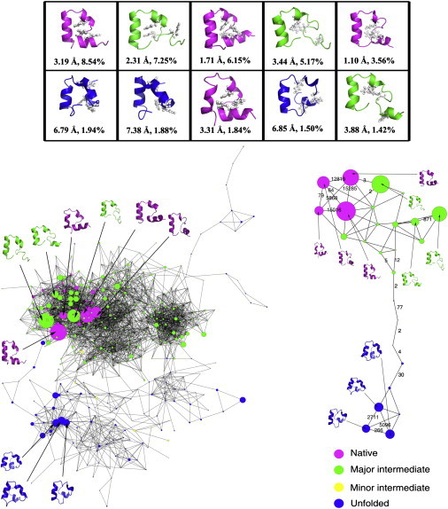
Folding network of trajectory WTP. (A) Representative structures of the 10 clusters with the highest population. The structures are colored by the folding states (purple for the folded state, green for the major intermediate state, yellow for the minor intermediate state, and blue for the unfolded state). The three hydrophobic core residues (residues F6, F10, and F17) are shown in ball-and-stick representation. Below the structures are the structural properties, including the overall Cα-RMSD and population of the cluster. (B) The fully connected folding network. Nodes are colored according to the folding state of each cluster. (C) A simplified minimal folding network that includes the top 10 nodes. Nodes are colored according to the folding state of each cluster. Transition numbers between selected pairs of nodes are also shown.
Diverse sampling of conformations within each folding state was observed among the top 10 clusters. Within the native state, although both segments were folded to <2.0 Å, the four clusters displayed distinctive characteristics. Clusters 3 and 5 had subangstrom folding in both segments, and thus good overall folding (1.71 Å and 1.10 Å, respectively). The individual helices were better formed in cluster 3, but the overall RMSD was smaller in cluster 5 due to the more native-like orientation of the helices and the better native packing of the hydrophobic core (0.96 Å RMSD for cluster 5, and 1. 36 Å for cluster 3). The larger RMSD in cluster 1 (3.19 Å) was caused by the nonnative planer arrangement in segment A and bad packing of the hydrophobic core (2.77 Å RMSD), whereas the larger RMSD in cluster 8 (3.31 Å) was caused by the nonideal helix formation in segment B (1.56 Å RMSD). Within the intermediate state, the difference in segment A was even more pronounced (from 2.54 Å in cluster 2, to 3.73 Å in cluster 4 and 4.58 Å in cluster 10). Although the folding of segment B was very good in cluster 2 and the overall folding was decent (2.31 Å RMSD), it still belonged to the intermediate state because of the poor formation of helix I. The less well-folded segment B, together with the poor formation of helix I and the helix I-II linker region led to a larger overall RMSD in clusters 4 and 10 (3.44 Å and 3.88 Å, respectively). In addition, F6 was far away from F10 and F17 for all those three nodes, leading to a large RMSD for the hydrophobic core (>4.77 Å). Within the unfolded state, all three clusters had helix I pointing in the wrong direction, leading to very large RMSD in segment A (>5.11 Å) and the hydrophobic core (>4.38 Å). In addition, this wrongly oriented helix I also interfered with the folding of segment B, leading to wider separation of helices II and III and a large RMSD in segment B (>3.74 Å). Overall, the very large global RMSD (>6.79 Å) in the unfolded state was mainly caused by the nonnative packing of the three helices.
Based on the above-mentioned clustering and the detection of transitions among the clusters, we constructed a folding network (Fig. 2 B). Among the 468 clusters, there were 29 clusters in the native state with a combined population of 29.6%, 291 clusters in the major intermediate state with a combined population of 52.3%, 12 clusters in the minor intermediate state with a combined population of 0.9%, and 136 clusters in the unfolded state with a combined population of 17.2%. The color of each node was based on the folding-state assignment of the cluster center, and the size of each node was based on the population of the cluster. In addition, the structures of the 10 largest nodes were illustrated on the network.
Based on the network topology, we concluded that the folding network consisted of two modules (i.e., interconnected groups of clusters): a dense module at the top and a loose module at the bottom. The distribution of folding states was very clear on this network. The native conformations and major intermediate conformations were at the top, whereas the unfolded conformations and a few minor intermediate conformations were mostly at the bottom. The good separation of folding states suggested a flow of conformations from the unfolded state to the major intermediate state and finally to the folded state. Of interest, the native conformations and major intermediate conformations were not well separated, indicating frequent transitions between the two states. In fact, we observed 4629 transitions between these two states (balanced in both directions), but much fewer transitions between any other pairs of states. The high connectivity between the native and the major intermediate states suggested that the clear separation of the two states on the 2D landscape may not be an accurate depiction of the real folding landscape of HP35. Further examination of the network revealed more details about the folding mechanism. The mixing of the minor intermediate conformations with the unfolded conformations suggested that the minor intermediate state is an off-pathway intermediate state. More importantly, multiple routes of transitions between the unfolded conformations and major intermediate conformations were observed, suggesting heterogeneity in the folding/unfolding of HP35.
Since the top 10 nodes accounted for nearly 40% of the total population, a minimal network connecting the top 10 nodes would be an informative representation of the entire network. High intrastate connectivity was observed in this minimal network (Fig. 2 C). The three nodes at the unfolded state were directly interconnected, as were the four nodes at the native state and two of the three nodes at the major intermediate state. The four nodes at the native state were clustered together but had connections with several surrounding nodes at the major intermediate state. The nodes at the unfolded state were all clustered together and had only one connection with the major intermediate state. It was also evident that the intrastate transitions significantly outnumbered the interstate transitions. Consistent with the full network, this minimal network demonstrated a good connection between the native state and the major intermediate state, and isolation of the unfolded state from those two states.
Folding networks of the other four trajectories
As with many other descriptions of protein folding, a folding network should not be overinterpreted on the basis of a single folding trajectory. To demonstrate this, we constructed folding networks based on the other four trajectories. In comparison with the above-described network, we observed both similarities and differences.
Among the top 10 nodes in trajectory WTC (Fig. 3 A), there were eight clusters at the major intermediate state and two clusters at the native state, whereas both the unfolded and minor intermediate states were absent due to the lower population. Consistent with trajectory WTP, conformational heterogeneity was observed within both the native and major intermediate states. The folding network mainly consisted of two modules (Fig. 3 B). The upper-right portion of the network was a loosely connected module at the unfolded state. The lower-left portion was a densely connected module mostly at the native or major intermediate state. The relatively good separation between the unfolded state and the other two states was consistent with trajectory WTP. The major deviation was the significantly higher population in the major intermediate state. In addition, the mixing of a few unfolded conformations with major intermediate conformations was observed at the left corner of the network. Among the top 10 nodes, the two native conformations and seven of the eight major intermediate conformations had direct intrastate transitions (Fig. 3 C). The minimal network connecting the top 10 nodes again demonstrated that the native state was imbedded in the major intermediate state. Due to the much longer distance from the top 10 nodes, none of the unfolded conformations were included in this minimal network, further supporting the separation of unfolded state from those two states.
Figure 3.

Folding network of trajectory WTC. For details, refer to the legend of Fig. 2.
In trajectory WTF, the major intermediate conformations were absent from the top 10 list due to the low population (Fig. 4 A). The top 10 nodes consisted of nine unfolded conformations and one native conformation. Structural heterogeneity was also observed among the nine unfolded conformations. The folding network consisted of two modules (Fig. 4 B): a module with only unfolded conformations on the right, and another module on the left with mixed native and major intermediate conformations. The minimal network suggested the clear transition from the unfolded state to the major intermediate state and then the native state (Fig. 4 C). The good separation of the unfolded state from the other two states was evident from the minimal network. In addition, the top nine unfolded nodes had high intrastate connectivity, which is consistent with the network features from the other two trajectories.
Figure 4.

Folding network of trajectory WTF. For details, refer to the legend of Fig. 2.
The unfolded state was also highly populated in trajectory WTI (Fig. 5 A). The top 10 nodes consisted of four unfolded conformations (total population 43.9%), four major intermediate conformation (total population 4.78%), and two native conformations (total population 4.30%). The folding network mainly consisted of four modules (Fig. 5 B): three on the left with mostly unfolded nodes and a few small minor intermediate nodes, and one highly connected module on the right with the major intermediate and native nodes. The mixing of the major intermediate and native nodes, and the good separation from the unfolded node can also be clearly seen on the minimal network (Fig. 5 C).
Figure 5.

Folding network of trajectory WTI. For details, refer to the legend of Fig. 2.
The top 10 nodes of trajectory WTK consisted of four major intermediate nodes (total population 11.68%), three native nodes (total population 10.27%), and three unfolded nodes (total population 5.56%) (Fig. 6 A). The folding network mainly consisted of three modules: two small ones on the left with unfolded nodes, and a large one on the right with mixed native and major intermediate nodes (Fig. 6 B). This feature is also reflected on the minimal network (Fig. 6 C).
Figure 6.

Folding network of trajectory WTK. For details, refer to the legend of Fig. 2.
Discussion
Comparison with classical theories of protein folding
To further dissect the folding events, we conducted analyses on the partial folding of the protein, including segment folding, hydrophobic core formation, turn formation, and formation of the individual helices (for details, see the Supporting Material). Here we describe the main observations from those analyses and compare them with general theories of protein folding.
In trajectory WTP, the Cα-RMSD profile of segment A (residues 2–20, encompassing helices I and II) was very similar to the global Cα-RMSD profile. However, the Cα-RMSD profile of segment B (residues 13–31, encompassing helices II and III) was below 2.0 Å during the majority of the simulation time. A similar feature was observed in other trajectories, although segment B unfolded after ∼2 μs in trajectory WTF. This indicated that the folding of segment B was faster and more robust, whereas the dynamics in segment A led to the fluctuation of global Cα-RMSD. This observation is consistent with the diffusion-collision theory proposed by Karplus and Weaver (40), which holds that protein folding is guided by the diffusion and collision of prefolded secondary structure elements. In the case of HP35, the prefolded helices II and III collide with each other and form folded segment B, which then collides with the prefolded helix I and forms the globally folded HP35.
We then examined the formation of the individual helices. In trajectory WTP, the first two hydrogen bonds in helix III and the middle two hydrogen bonds in helix I had significantly higher occupancy than the neighboring hydrogen bonds. A similar feature was observed in other trajectories. This suggests that these helical turns may be critical for HP35 folding. The initiation of folding from the formation of helical turns is consistent with the nucleation-condensation theory (41). According to our simulation, the folding of HP35 initiated from the N-terminal of helix III and the middle of helix I, which formed two folding nuclei. This subsequently propagated to the formation of individual helices, followed by the diffusion and collision step. In a way, these two major folding theories were unified in the folding of HP35 from our simulation.
To compare our results with the hydrophobic-hydration theory (42), we investigated the formation of the hydrophobic core by three phenylalanine residues: F6, F10, and F17. In trajectory WTP, the hydrophobic core RMSD profile followed a fluctuation pattern similar to that of the global Cα-RMSD and the Cα-RMSD of segment A, in contrast to the much more stable pattern of the Cα-RMSD of segment B. A similar feature was observed in other trajectories. This suggests that the formation of this hydrophobic core is not the driving force behind HP35 folding, perhaps because of the relatively small hydrophobic cluster formed by the three phenylalanine residues.
Analyses of energetics
To further investigate the driving force of the folding, we calculated the average potential energy (including the solvation free energy) of the top 10 clusters (Fig. 2). In trajectory WTP, the native conformations had the highest average potential energy (−622.67 kcal/mol, −620.27 kcal/mol, −624.90 kcal/mol, and −621.33 kcal/mol for clusters 1, 3, 5, and 8, respectively), the unfolded conformations had the lowest average potential energy (−629.23 kcal/mol, −627.51 kcal/mol, and −631.35 kcal/mol for clusters 6, 7 and 9, respectively), and the average potential energy of the major intermediate conformations was in between (−625.85 kcal/mol, −625.05 kcal/mol, and −624.00 kcal/mol for clusters 2, 4, and 10, respectively). A similar trend was observed in trajectories WTC and WTF.
The lower potential energy in the unfolded state was likely due to the higher compactness (data not shown). In trajectory WTP, the least compact conformation among the top 10 clusters was a major intermediate conformation (cluster 10) with 3327 Å2 total accessible surface area, and the most compact conformation was an unfolded conformation (cluster 9) with 3072 Å2 total accessible surface area. Another unfolded conformation (cluster 7) had the second-lowest accessible surface area (3123 Å2). A similar trend was observed in other trajectories. Higher compactness led to more atom contact and lower potential energy. However, the overall correlation between potential energy and accessible surface area was not strong (data not shown).
We also investigated the energy distribution on the network by using the average potential energy of clusters for color-coding (see Supporting Material). In trajectory WTP, the more-populated nodes generally had lower potential energy (<−619 kcal/mol). Among the lower-energy nodes, the larger nodes at the bottom (unfolded conformations) had the lowest potential energy (<−626 kcal/mol), and most of the larger nodes on the top (native or major intermediate conformations) had slightly higher potential energy (−626 to −619 kcal/mol). A similar trend was observed in other trajectories.
Comparison with recent findings from experiments
To further reveal the energy barriers on the folding landscape of HP35, we constructed 2D maps based on segment RMSD (see Supporting Material). From the 2D maps, we observed two free-energy barriers: a major one from the U state to the I1 state, which corresponded to the folding of segment B; and a minor one from the I1 state to the N state, which corresponded to the subsequent folding of segment A. This is consistent with observations in our previous work (6,8).
We then examined the role of the second turn in the folding of segment B. In trajectory WTP, the turn RMSD profile was similar to that of segment B (see Supporting Material), indicating a high correlation between the turn formation and the folding of segment B with helices II and III connected by this turn. A more careful examination revealed that the turn formation was slightly ahead of the segment B folding, and the variation of the RMSD in segment B was higher than that of the turn. A similar feature was observed in other trajectories. This suggests that formation of the second turn may be critical for segment B folding, and likely constitutes the rate-limiting step. This is also consistent with observations in our previous work (6,8). However, we should note that, although HP35 reached the native state within 1 μs in some simulation trajectories, it is difficult to estimate the folding rate based on our simulation due to the limited number of simulation trajectories (20 in our previous work and five in this work).
HP35 is one of the most studied proteins in the field of protein folding. We have reviewed some of the notable studies in our previous works (6,8). Some of the predictions we made in those studies regarding the folding mechanism were subsequently verified by experiments. In an unfolding study using fluorescence resonance energy transfer, Glasscock and co-workers (43) demonstrated that the turn linking helices II and III remains compact under the denaturation condition, suggesting that the unfolding of HP35 consists of multiple steps and starts with the unfolding of helix I. In a mutagenesis experiment, Bunagan et al. (44) showed that the second turn region plays an important role in the folding rate of HP35. A recent freeze-quenching experiment by Hu and co-workers (45) revealed an intermediate state with native secondary structures and nonnative tertiary contacts. These experiments are highly consistent with our observations in terms of both the stepwise folding and the rate-limiting step. Kubelka et al. (46) proposed a three-state model in which the interconversion between the intermediate state and folded state is much faster than that between the intermediate state and the unfolded state. Therefore, the intermediate state lies on the folded side of the major free-energy barrier, which is consistent with the separation of the unfolded state from the other two states in our folding network. The estimation of 1.6–2.0 kcal/mol for the major free-energy barrier is also consistent with the estimation from our previous REMD simulation (47).
Nevertheless, controversy still exists regarding the folding mechanism of this small protein. In a recent work by Reiner et al. (48), a folded segment with helices I/II was proposed as the intermediate state, which corresponds to the off-pathway minor intermediate state in our work. It should be noted that different perturbations to the system, including high concentrations of denaturant, high temperatures, and site mutagenesis, have been utilized in different folding experiments. Because of the small size of HP35, the folding process may be sensitive to some of these perturbations. With the continuous development of experimental techniques that allow minimal perturbation and monitoring of the folding process at higher spatial and temporal resolution, the protein-folding mechanism will become more and more clear.
Comparison with other representations of protein folding
Because of the large number of degrees of freedom involved in protein folding, it is inevitably a multidimensional process that is difficult to represent. The most widely used property to describe protein folding has been the RMSD (either global or local). In general, the RMSD is a good indicator of the closeness between two structures. However, the RMSD is a degenerated numerical property. For a protein, one RMSD value may correspond to many different conformations. The same is true for other properties, such as the potential energy, solvent-accessible surface area, and helicity. Therefore, when these properties are used to describe the folding process, the exact conformational transitions cannot be fully represented. When two of these properties are combined to construct a 2D map, even though the degeneracy is significantly reduced, a spot on the map may still correspond to multiple conformations, leading to ambiguity in the interpretation of the results. Thus, novel representations that reflect the multidimensional nature of protein folding are needed.
The disconnectivity graph published by Krivov and Karplus (12) and the folding network developed by Rao and Caflisch (16) are both promising techniques for obtaining a multidimensional description of protein folding. The former mainly emphasizes energy, whereas the latter focuses more on conformation. Recently, Jiang et al. (49) applied a Markov cluster algorithm to a folding analysis of the trpzip2 peptide. A simplified network with five basins was constructed and the relative free energy and interbasin transitions were clearly demonstrated. In another work, Rajan et al. (50) applied a principle component analysis (PCA) and a nonmetric multidimensional scaling method to a folding analysis of HP35. The analysis greatly reduced the dimensionality of the simulation data and revealed the hidden structural heterogeneity. Recently, Hori and co-workers (51) used PCA to study the folding of protein G and src SH3. The results revealed a funnel-shaped folding landscape, especially toward the end of the folding process. The folding network was characterized as hierarchical with scale-free and small-world properties. We also conducted a PCA of HP35 folding in our previous work (6,8). Here, we adopted the network technique to reflect the conformational space in a fully connected network, and added folding state and energy information to the network. This combination provided detailed information and what we believe are new insights about the folding of HP35.
Our main observation from the RMSD profiles is that the fast folding and high stability of segment B plays an important role in the folding of HP35. However, it was rather challenging to visualize the conformational change from the RMSD curves. This situation was significantly improved in the 2D map, where the four folding states were clearly separated and the folding mechanism became clear. However, this representation still oversimplified the real protein folding process. The folding network, on the other hand, provided more detailed information. In contrast to the concentrated regions on the 2D map, many conformations were observed in every folding state on the folding network. In addition, the conformational transitions could be visualized in the form of a connected network. The use of different colors for the network nodes, such as the folding states, demonstrated the distribution of different properties throughout the network. Zooming-up of the network provided even more detailed information, such as the conformational transition pathway and the number of transitions between any pair of nodes. We conclude that the combination of traditional and network analyses can provide a better understanding of the folding mechanism.
Conclusions
We conducted a network analysis of the reversible folding of HP35 in a set of 10 μs folding trajectories. Compared with the classical 2D folding landscape, the folding network uncovered more intrinsic complexity of the folding landscape. Structural heterogeneity was observed in each of the folding states, including the unfolded state, intermediate state, and even the native state. Several groups of conformations were clearly distinguishable yet linked together. Energetic analyses revealed deep enthalpic traps at the unfolded state. In addition, the mixing of the native conformations and major intermediate conformations on the network was different from the clear separation of the two states on the 2D folding landscape. In summary, comprehensive network analyses of protein folding can provide new insights into the folding mechanism.
Acknowledgments
Usage of AMBER and Pymol, GRACE, VMD, MATLAB, and Rasmol graphics packages is gratefully acknowledged.
This work was supported by research grants from the National Institutes of Health (GM79383 and GM67168 to Y.D.), the National Natural Science Foundation of China (30870474 to H.L.), and the Scientific Research Foundation for Returned Overseas Chinese Scholars, State Education Ministry (to H.L.). The research was also supported in part by the Project of Knowledge Innovation Program of the Chinese Academy of Sciences (grant KJCX2.YW.W10).
Contributor Information
Hongxing Lei, Email: leihx@big.ac.cn.
Yong Duan, Email: duan@ucdavis.edu.
Supporting Material
References
- 1.Bryngelson J.D., Onuchic J.N., Wolynes P.G. Funnels, pathways, and the energy landscape of protein folding: a synthesis. Proteins. 1995;21:167–195. doi: 10.1002/prot.340210302. [DOI] [PubMed] [Google Scholar]
- 2.Herges T., Wenzel W. Free-energy landscape of the villin headpiece in an all-atom force field. Structure. 2005;13:661–668. doi: 10.1016/j.str.2005.01.018. [DOI] [PubMed] [Google Scholar]
- 3.Liu F., Dumont C., Gruebele M. A one-dimensional free energy surface does not account for two-probe folding kinetics of protein α D-3. J. Chem. Phys. 2009;130:061101. doi: 10.1063/1.3077008. [DOI] [PMC free article] [PubMed] [Google Scholar]
- 4.Zagrovic B., Snow C.D., Pande V.S. Simulation of folding of a small α-helical protein in atomistic detail using worldwide-distributed computing. J. Mol. Biol. 2002;323:927–937. doi: 10.1016/s0022-2836(02)00997-x. [DOI] [PubMed] [Google Scholar]
- 5.Corcho F.J., Mokoena P., Perez J.J. Molecular dynamics (MD) simulations of VIP and PACAP27. Biopolymers. 2009;91:391–400. doi: 10.1002/bip.21147. [DOI] [PubMed] [Google Scholar]
- 6.Lei H., Duan Y. Two-stage folding of HP-35 from ab initio simulations. J. Mol. Biol. 2007;370:196–206. doi: 10.1016/j.jmb.2007.04.040. [DOI] [PMC free article] [PubMed] [Google Scholar]
- 7.Lei H., Duan Y. Ab initio folding of albumin binding domain from all-atom molecular dynamics simulation. J. Phys. Chem. B. 2007;111:5458–5463. doi: 10.1021/jp0704867. [DOI] [PubMed] [Google Scholar]
- 8.Lei H., Wu C., Duan Y. Folding free-energy landscape of villin headpiece subdomain from molecular dynamics simulations. Proc. Natl. Acad. Sci. USA. 2007;104:4925–4930. doi: 10.1073/pnas.0608432104. [DOI] [PMC free article] [PubMed] [Google Scholar]
- 9.Lei H.X., Wang Z.X., Duan Y. Dual folding pathways of an α/β protein from all-atom ab initio folding simulations. J. Chem. Phys. 2009;131:165105. doi: 10.1063/1.3238567. [DOI] [PMC free article] [PubMed] [Google Scholar]
- 10.Lei H.X., Wu C., Duan Y. Folding processes of the B domain of protein A to the native state observed in all-atom ab initio folding simulations. J. Chem. Phys. 2008;128:235105. doi: 10.1063/1.2937135. [DOI] [PMC free article] [PubMed] [Google Scholar]
- 11.Qi Y.F., Huang Y.Q., Lai L. Folding simulations of a de novo designed protein with a βαβ fold. Biophys. J. 2010;98:321–329. doi: 10.1016/j.bpj.2009.10.018. [DOI] [PMC free article] [PubMed] [Google Scholar]
- 12.Krivov S.V., Karplus M. Free energy disconnectivity graphs: application to peptide models. J. Chem. Phys. 2002;117:10894–10903. [Google Scholar]
- 13.Krivov S.V., Karplus M. Hidden complexity of free energy surfaces for peptide (protein) folding. Proc. Natl. Acad. Sci. USA. 2004;101:14766–14770. doi: 10.1073/pnas.0406234101. [DOI] [PMC free article] [PubMed] [Google Scholar]
- 14.Palla G., Derényi I., Vicsek T. Uncovering the overlapping community structure of complex networks in nature and society. Nature. 2005;435:814–818. doi: 10.1038/nature03607. [DOI] [PubMed] [Google Scholar]
- 15.Duan Y., Kollman P.A. Pathways to a protein folding intermediate observed in a 1-microsecond simulation in aqueous solution. Science. 1998;282:740–744. doi: 10.1126/science.282.5389.740. [DOI] [PubMed] [Google Scholar]
- 16.Rao F., Caflisch A. The protein folding network. J. Mol. Biol. 2004;342:299–306. doi: 10.1016/j.jmb.2004.06.063. [DOI] [PubMed] [Google Scholar]
- 17.Caflisch A. Network and graph analyses of folding free energy surfaces. Curr. Opin. Struct. Biol. 2006;16:71–78. doi: 10.1016/j.sbi.2006.01.002. [DOI] [PubMed] [Google Scholar]
- 18.Muff S., Caflisch A. Kinetic analysis of molecular dynamics simulations reveals changes in the denatured state and switch of folding pathways upon single-point mutation of a β-sheet miniprotein. Proteins. 2008;70:1185–1195. doi: 10.1002/prot.21565. [DOI] [PubMed] [Google Scholar]
- 19.Hansmann U.H. Simulations of a small protein in a specifically designed generalized ensemble. Phys. Rev. E. 2004;70:012902. doi: 10.1103/PhysRevE.70.012902. [DOI] [PubMed] [Google Scholar]
- 20.Hansmann U.H.E., Okamoto Y. Generalized-ensemble Monte Carlo method for systems with rough energy landscape. Phys. Rev. E. 1997;56:2228–2233. [Google Scholar]
- 21.Kubelka J., Eaton W.A., Hofrichter J. Experimental tests of villin subdomain folding simulations. J. Mol. Biol. 2003;329:625–630. doi: 10.1016/s0022-2836(03)00519-9. [DOI] [PubMed] [Google Scholar]
- 22.Chiu T.K., Kubelka J., Davies D.R. High-resolution x-ray crystal structures of the villin headpiece subdomain, an ultrafast folding protein. Proc. Natl. Acad. Sci. USA. 2005;102:7517–7522. doi: 10.1073/pnas.0502495102. [DOI] [PMC free article] [PubMed] [Google Scholar]
- 23.Reference deleted in proof.
- 24.Duan Y., Wang L., Kollman P.A. The early stage of folding of villin headpiece subdomain observed in a 200-nanosecond fully solvated molecular dynamics simulation. Proc. Natl. Acad. Sci. USA. 1998;95:9897–9902. doi: 10.1073/pnas.95.17.9897. [DOI] [PMC free article] [PubMed] [Google Scholar]
- 25.De Mori G.M., Colombo G., Micheletti C. Study of the villin headpiece folding dynamics by combining coarse-grained Monte Carlo evolution and all-atom molecular dynamics. Proteins. 2005;58:459–471. doi: 10.1002/prot.20313. [DOI] [PubMed] [Google Scholar]
- 26.Shen M.Y., Freed K.F. All-atom fast protein folding simulations: the villin headpiece. Proteins. 2002;49:439–445. doi: 10.1002/prot.10230. [DOI] [PubMed] [Google Scholar]
- 27.Zagrovic B., Snow C.D., Pande V.S. Native-like mean structure in the unfolded ensemble of small proteins. J. Mol. Biol. 2002;323:153–164. doi: 10.1016/s0022-2836(02)00888-4. [DOI] [PubMed] [Google Scholar]
- 28.Pande V.S., Baker I., Zagrovic B. Atomistic protein folding simulations on the submillisecond time scale using worldwide distributed computing. Biopolymers. 2003;68:91–109. doi: 10.1002/bip.10219. [DOI] [PubMed] [Google Scholar]
- 29.Jayachandran G., Vishal V., Pande V.S. Using massively parallel simulation and Markovian models to study protein folding: examining the dynamics of the villin headpiece. J. Chem. Phys. 2006;124:164902. doi: 10.1063/1.2186317. [DOI] [PubMed] [Google Scholar]
- 30.Jang S., Kim E., Pak Y. Ab initio folding of helix bundle proteins using molecular dynamics simulations. J. Am. Chem. Soc. 2003;125:14841–14846. doi: 10.1021/ja034701i. [DOI] [PubMed] [Google Scholar]
- 31.Ripoll D.R., Vila J.A., Scheraga H.A. Folding of the villin headpiece subdomain from random structures. Analysis of the charge distribution as a function of pH. J. Mol. Biol. 2004;339:915–925. doi: 10.1016/j.jmb.2004.04.002. [DOI] [PubMed] [Google Scholar]
- 32.Carr J.M., Trygubenko S.A., Wales D.J. Finding pathways between distant local minima. J. Chem. Phys. 2005;122:234903. doi: 10.1063/1.1931587. [DOI] [PubMed] [Google Scholar]
- 33.Wen E.Z., Hsieh M.J., Luo R. Enhanced ab initio protein folding simulations in Poisson-Boltzmann molecular dynamics with self-guiding forces. J. Mol. Graph. Model. 2004;22:415–424. doi: 10.1016/j.jmgm.2003.12.008. [DOI] [PubMed] [Google Scholar]
- 34.Lee I.H., Kim S.Y., Lee J. Dynamic folding pathway models of the villin headpiece subdomain (HP-36) structure. J. Comput. Chem. 2010;31:57–65. doi: 10.1002/jcc.21288. [DOI] [PubMed] [Google Scholar]
- 35.Case D.A., Cheatham T.E., 3rd, Woods R.J. The Amber biomolecular simulation programs. J. Comput. Chem. 2005;26:1668–1688. doi: 10.1002/jcc.20290. [DOI] [PMC free article] [PubMed] [Google Scholar]
- 36.Duan Y., Wu C., Kollman P. A point-charge force field for molecular mechanics simulations of proteins based on condensed-phase quantum mechanical calculations. J. Comput. Chem. 2003;24:1999–2012. doi: 10.1002/jcc.10349. [DOI] [PubMed] [Google Scholar]
- 37.Onufriev A., Bashford D., Case D.A. Exploring protein native states and large-scale conformational changes with a modified generalized Born model. Proteins. 2004;55:383–394. doi: 10.1002/prot.20033. [DOI] [PubMed] [Google Scholar]
- 38.Berendsen H.J.C., Postma J.P.M., Haak J.R. Molecular-dynamics with coupling to an external bath. J. Chem. Phys. 1984;81:3684–3690. [Google Scholar]
- 39.Ryckaert J.P., Ciccotti G., Berendsen H.J.C. Numerical integration of Cartesian equations of motion of a system with constraints—molecular-dynamics of N-alkanes. J. Comput. Phys. 1977;23:327–341. [Google Scholar]
- 40.Karplus M., Weaver D.L. Protein folding dynamics: the diffusion-collision model and experimental data. Protein Sci. 1994;3:650–668. doi: 10.1002/pro.5560030413. [DOI] [PMC free article] [PubMed] [Google Scholar]
- 41.Fersht A.R. Optimization of rates of protein folding: the nucleation-condensation mechanism and its implications. Proc. Natl. Acad. Sci. USA. 1995;92:10869–10873. doi: 10.1073/pnas.92.24.10869. [DOI] [PMC free article] [PubMed] [Google Scholar]
- 42.Dill K.A. Dominant forces in protein folding. Biochemistry. 1990;29:7133–7155. doi: 10.1021/bi00483a001. [DOI] [PubMed] [Google Scholar]
- 43.Glasscock J.M., Zhu Y., Gai F. Using an amino acid fluorescence resonance energy transfer pair to probe protein unfolding: application to the villin headpiece subdomain and the LysM domain. Biochemistry. 2008;47:11070–11076. doi: 10.1021/bi8012406. [DOI] [PMC free article] [PubMed] [Google Scholar]
- 44.Bunagan M.R., Gao J., Gai F. Probing the folding transition state structure of the villin headpiece subdomain via side chain and backbone mutagenesis. J. Am. Chem. Soc. 2009;131:7470–7476. doi: 10.1021/ja901860f. [DOI] [PMC free article] [PubMed] [Google Scholar]
- 45.Hu K.N., Yau W.M., Tycko R. Detection of a transient intermediate in a rapid protein folding process by solid-state nuclear magnetic resonance. J. Am. Chem. Soc. 2010;132:24–25. doi: 10.1021/ja908471n. [DOI] [PMC free article] [PubMed] [Google Scholar]
- 46.Kubelka J., Henry E.R., Eaton W.A. Chemical, physical, and theoretical kinetics of an ultrafast folding protein. Proc. Natl. Acad. Sci. USA. 2008;105:18655–18662. doi: 10.1073/pnas.0808600105. [DOI] [PMC free article] [PubMed] [Google Scholar]
- 47.Godoy-Ruiz R., Henry E.R., Eaton W.A. Estimating free-energy barrier heights for an ultrafast folding protein from calorimetric and kinetic data. J. Phys. Chem. B. 2008;112:5938–5949. doi: 10.1021/jp0757715. [DOI] [PubMed] [Google Scholar]
- 48.Reiner, A., P. Henklein, and T. Kiefhaber. An unlocking/relocking barrier in conformational fluctuations of villin headpiece subdomain. Proc. Natl. Acad. Sci. USA 107:4955–4960. [DOI] [PMC free article] [PubMed]
- 49.Jiang X.W., Chen C.J., Xiao Y. Improvements of network approach for analysis of the folding free-energy surface of peptides and proteins. J. Comput. Chem. 2010;31:57–65. doi: 10.1002/jcc.21544. [DOI] [PubMed] [Google Scholar]
- 50.Rajan A., Freddolino P.L., Schulten K. Going beyond clustering in MD trajectory analysis: an application to villin headpiece folding. PLoS ONE. 2010;5:e9890. doi: 10.1371/journal.pone.0009890. [DOI] [PMC free article] [PubMed] [Google Scholar]
- 51.Hori N., Chikenji G., Takada S. Folding energy landscape and network dynamics of small globular proteins. Proc. Natl. Acad. Sci. USA. 2009;106:73–78. doi: 10.1073/pnas.0811560106. [DOI] [PMC free article] [PubMed] [Google Scholar]
Associated Data
This section collects any data citations, data availability statements, or supplementary materials included in this article.