Dynamic energy budget theory restores coherence in biology

Abstract

We present the state of the art of the development of dynamic energy budget theory, and its expected developments in the near future within the molecular, physiological and ecological domains. The degree of formalization in the set-up of the theory, with its roots in chemistry, physics, thermodynamics, evolution and the consistent application of Occam's razor, is discussed. We place the various contributions in the theme issue within this theoretical setting, and sketch the scope of actual and potential applications.

1. Reaching out for generality

In physics, there is a quest for a unified theory. Physical theories have a broad spectrum of application, a strong mathematical background and are subject to numerous empirical tests. By contrast, in biology, mathematical theory has played a secondary role because biology is frequently seen as a science of exceptions and particular cases, with little interest in abstraction and generalization. Exceptions are the research being done in the fields of theoretical biology and mathematical biology. However, theoretical and mathematical biology have frequently been carried out without a concern for empirical testing. When this concern appears, models are of narrow application, reducing their theoretical breadth. The dynamic energy budget (DEB) theory starts from the Dutch tradition of theoretical and mathematical biology, but couples it with a fundamental concern in producing general theory that is subjected to careful empirical testing.

DEB theory aims to capture the quantitative aspects of metabolism at the individual level for organisms of all species. It builds on the premise that the mechanisms that are responsible for the organization of metabolism are not species-specific (Kooijman 2001, 2010). This hope for generality is supported by (i) the universality of physics and evolution and (ii) the existence of widespread biological empirical patterns among organisms (Sousa et al. 2008). Table 1 synthesizes the essential criteria for any general model for the metabolism of individuals. We explore the links between DEB theory and each of the proposed criteria in the following paragraphs.

Table 1.

Criteria for general explanatory models for the energetics of individuals.

1. consistency with other scientific knowledge: the models must be based on explicit assumptions that are consistent with thermodynamics, physics, (geo)chemistry and evolution.

2. consistency with empirical data: the assumptions should be consistent with empirical patterns.

3. life-cycle approach: the assumptions should cover the full life cycle of the individual, from initiation of development to death.

4. Occam's razor: the general model should be as simple as possible (and not more). The predictions should be testable in practice, which typically constrains its maximum complexity substantially (quantified in terms of number of variables and parameters).

5. taxon-specific adaptations: restrictions that make a model applicable to particular taxa only, should: (a) be consistent with an explicit evolutionary scenario; (b) be explicit to allow the prediction that the model will apply to those species.

DEB theory is explicitly based on the conservation of mass, isotopes, energy and time, including the inherent degradation of energy associated with all processes. So it complies to criteria 1, table 1.

The DEB theory is biologically implicit, so it applies to all species. Species-specific restrictions of DEB models are explained and predicted by the theory (criterion 5, table 1). For example, consider the most important difference between DEB models, the number of reserves (biomass components that fuel metabolism) and structures (biomass components that have maintenance needs) that are delineated. This depends on the degree of coupling of the various substrates an organism needs. Animals feed on other organisms, which couples uptake of the various substrates (proteins, carbohydrates, lipids, nutrients) tightly and explains why a single reserve and structure is appropriate for them. This does not hold for plants, for instance, where multiple reserves and structures (root, shoot) are required. This means that the applicability of a model can be judged a priori.

The structure of DEB theory is such that there is a smooth merging and splitting of reserves and structures, which is a key feature in response to evolutionary changes in acquisition strategies (Kooijman et al. 2003; Kooijman 2004, 2010; Kooijman & Hengeveld 2005; Troost et al. 2005; Kooijman & Troost 2007). It is possible to smoothly convert one DEB model into another, according to an evolutionary scenario that makes DEB species-specific models consistent with an evolutionary scenario (criterion 5, table 1). This includes organisms that evolved from the merging of ancestors such as the mitochondria and chloroplasts that once had an independent existence, and many of the symbioses (e.g. corals) that exist today.

In an attempt to be explicit on consistency with empirical observations (criterion 2, table 1), we organized generally observed patterns in empirical data on various aspects of energetics, life stages and stoichiometry in tables 2 and 3 (Sousa et al. 2006). DEB theory has an explanation for each of them. Many empirical models, such as Droop's model for the nutrient limited growth of algae and Huggett and Widdas' model for foetal growth, are special cases of DEB theory (table 4). The large collection of empirical support for all these findings that accumulated in the literature and the bits of evidence that people working with DEB accumulated during the 30 years of DEB research makes DEB theory presently the best tested quantitative theory in biology (Kooijman 2010).

Table 2.

Stylized facts and empirical evidence on feeding, growth, reproduction, respiration and death.

	stylized facts	empirical evidence
feeding	during starvation, organisms are able to reproduce	animals: Kjesbu et al. (1991), Hirche & Kattner (1993) and Kirk (1997)
	during starvation, organisms are able to grow	animals: Stromgren & Cary (1984), Russell & Wootton (1992), Roberts et al. 2001, Dou et al. (2002), Gallardo et al. (2004) and Zheng et al. (2005)
	during starvation, organisms are able to survive for some time	animals: Stockhoff (1991) and Letcher et al. (1996)
		bacteria: Kunji et al. (1993)
growth	the growth of isomorphic organisms at abundant food is well described by the von Bertalanffy growth curve  Putter (1920) and von Bertalanffy (1938)	animals: Frazer et al. (1990), Strum (1991), Chen et al. (1992), Schwartz & Hundertmark (1993), Ferreira & Russ (1994) and Ross et al. (1995)
	for different constant food levels the inverse von Bertalanffy growth rate increases linearly with ultimate length Putter (1920)	animals: Summers (1971), Galluci & Quinn (1979), Weindruch et al. (1986), Hubert et al. (2000) and Kooijman (2010, pp.48)
	many species do not stop growing after reproduction has started, i.e. they exhibit indeterminate growth Heino & Kaitala (1999) and Kozlowski (1996)	animals: Shine & Iverson (1995) and Jorgensen & Fiksen (2006)
	holometabolic insects are an exception foetuses increase in weight approximately proportional to cubed time Huggett & Widdas (1951)	animals: Huggett & Widdas (1951) and Zonneveld & Kooijman (1993)
	the von Bertalanffy growth rate of different species corrected for a common body temperature decreases almost proportional to maximum body length	bacteria: Kooijman (2000, pp. 276–282)
		yeasts: Kooijman (2000, pp. 276–282)
		animals: Kooijman (2000, pp. 276–282)
reproduction	reproduction increases with size intraspecifically but decreases with size interspecifically	animals: Peters (1983) and Kooijman (2010, pp. 69,323)
respiration	freshly laid eggs do not use dioxygen in significant amounts	animals: Whitehead (1987), Romijn & Lokhorst (1951), Pettit (1982) and Bucher (1983)
	the use of dioxygen increases with decreasing mass in embryos and increases with mass in juveniles and adults	animals: Romijn & Lokhorst (1951), Richman (1958), Pettit (1982), Bucher (1983), Whitehead (1987), Clarke & Johnston (1999) and Savage et al. (2004)
	the use of dioxygen scales approximately with body weight raised to a power close to 0.75 Kleiber (1932)	animals: Richman (1958), Clarke & Johnston 1999 and Savage et al. (2004)
	organisms show a transient increase in metabolic rate after ingesting food (heat increment of feeding)	animals: Janes & Chappell (1995), Chappell et al. (1997), Hawkins et al. (1997), Rosen & Trites (1997) and Nespolo et al. (2005)
ageing	lifespan increases with size for endotherms, but is independent of size in ectotherms	animals: Finch (1990) and Ricklefs & Finch (1995)

Table 3.

Stylized facts and empirical evidence on stoichiometry, energy dissipation and cells.

	stylized facts	empirical evidence
stoichiometry	chemical body composition of well- and poorly-fed organisms differ	animals: Hirche & Kattner (1993), Du & Mai (2004), Chen et al. (2005) and Molnar et al. (2006)
		yeasts: Hanegraaf et al. (2000)
	chemical body composition of organisms growing at constant food density becomes constant	animals: Chilliard et al. (2005), Krol et al. (2005), Fink et al. (2006), Ingenbleek (2006) and Steenbergen et al. (2006)
energy dissipation	dissipating heat is a weighted sum of three mass flows: carbon dioxide, dioxygen and nitrogenous waste	animals: Seale et al. (1991)
cells	cells in a tissue are metabolically very similar regardless the size of the organism Morowitz (1968)

Table 4.

Empirical models that turn out to be special cases of DEB models, or very good numerical approximations to them.

author	year	model
Lavoisier	1780	multiple regression of heat against mineral fluxes
Gompertz	1825	survival probability for ageing (Gompertz 1825)
Arrhenius	1889	temperature dependence of physiological rates
Huxley	1891	allometric growth of body parts (Huxley 1932)
Henri	1902	Michaelis Menten kinetics
Blackman	1905	bilinear functional response (Blackman 1905)
Hill	1910	Hill's functional response (Hill 1910)
Thornton	1917	heat dissipation (Thornton 1917)
Putter	1920	von Bertalanffy growth of individuals (Putter 1920)
Pearl	1927	logistic population growth (Pearl 1927)
Fisher and Tippitt	1928	Weibull aging (Fisher & Tippitt 1928)
Kleiber	1932	respiration scales with body weight raised to 3/4
Mayneord	1932	cube root growth of tumours (Mayneord 1932)
Monod	1942	growth of bacterial populations (Monod 1942)
Emerson	1950	cube root growth of bacterial colonies (Emerson 1950)
Huggett and Widdas	1951	foetal growth (Huggett & Widdas 1951)
Weibull	1951	survival probability for aging (Weibull 1951)
Best	1955	diffusion limitation of uptake (Best 1995)
Smith	1957	embryonic respiration (Smith 1957)
Leudeking and Piret	1959	microbial product formation (Leudeking & Piret 1959)
Holling	1959	hyperbolic functional response (Holling 1959)
Marr and Pirt	1962	maintenance in yields of biomass (Marr et al. 1963) and (Pirt 1965)
Droop	1973	reserve (cell quota) dynamics (Droop 1973, 1974, 1983)
Rahn and Ar	1974	water loss in bird eggs (Rahn & Ar 1974)
Hungate	1975	digestion (Hungate 1975)
Beer and Anderson	1997	development of salmonid embryos (Beer & Anderson 1997)

The pragmatic application of Occam's razor (criterion 4, table 1) in the construction of DEB theory privileged the smallest (possible) number of state variables, the smallest (possible) number of parameters, constant functions instead of linear and linear functions instead of nonlinear. For example, the variable stoichiometry of organisms, exposed to different food levels, is explained, in the DEB standard model, by describing biomass as two aggregated chemical compounds with constant chemical compositions and variable relative amounts.

Biomass is assumed to consist of one or more reserves and one or more structures. The dynamics of these metabolic pools is followed using five concepts of homeostasis, which are all meant for simplification and enhancing the testability of model predictions. The various forms of homeostasis are linked to the principle (criterion 1, table 1) that organisms have increased their control over metabolism during evolution allowing for some adaptation to environmental changes in short periods.

(a). Strong homeostasis

Metabolic pools do not change in composition and can be conceived as generalized compounds, i.e. mixtures of a large number of compounds of constant chemical composition and thermodynamic properties. The individual feeds on substrate (food, X) and produces products (faeces, water, carbon dioxide, ammonia, etc.), biomass (reserve E and structure V) and gametes (reserve allocated to reproduction). The standard DEB model (but not DEB models in general) assumes a fixed chemical composition for food. All (generalized) compounds have constant thermodynamic properties such as mass–energy couplers (chemical potentials) and mass–entropy couplers (specific entropies). Strong homeostasis imposes constant conversion coefficients on all aggregated chemical reactions occurring in the organism including assimilation, dissipation and growth, which comes with stoichiometric constraints. The combination of stoichiometric constraints and variations in the composition of biomass (reserve/structure ratio) leads to rather complex patterns at the various levels of organization.

(b). Weak homeostasis

The individual as a whole does not change in composition during growth in environments with constant food availability (possibly after an adaptation period). The composition (controlled by the ratio of reserve to structure) varies with the level of food availability. This implies constraints on the dynamics of reserve relative to structure.

(c). Structural homeostasis

The individual does not change the shape during growth, which controls how surface area relates to volume as they change in time. This simplifies the control of metabolism since some processes are proportional to surface area while others are proportional to volume. Transport processes, including food uptake, uptake and elimination of toxicants, osmosis and heat transfer, are proportional to surface area, which is compatible with the description of these processes in non-equilibrium thermodynamics (criterion 1, table 1). By contrast, most maintenance costs are linked to (structural) mass (turnover), so to volume. The scaling of feeding relative to maintenance controls ultimate body size. Only the standard DEB model makes use of structural homeostasis, not the wider class of uni- and multivariate DEB models.

(d). Acquisition homeostasis

The individual eats what it needs (demand systems), rather than what is available (supply systems). Species can be ranked on the supply–demand spectrum; no species can follow the demand rules into the extreme (food must obviously be available at some minimum level). All demand systems are animals that have typically a higher behavioural flexibility and a lower metabolic flexibility. Demand systems evolved from supply systems and most are endothermic.

(e). Thermal homeostasis

The individual (endotherms, mainly birds and mammals) heats the body to a constant temperature. This behaviour has an energetic cost, that might be significant under particular conditions, but it allows these species a higher independence over the environment since all metabolic rates depend on temperature.

The state variables of DEB theory are the structure(s), the reserve(s) and the level of maturity. The level of maturity controls life-stage transitions that cover the full life cycle of the organism (criterion 3, table 1).

Consistency with the evolutionary principle (criterion 1, table 1) that organisms inherit parents' characteristics in a sloppy way allowing for some adaptation to environmental changes across generations makes the set of parameter values in DEB individual-specific. Selection leads to evolution characterized by a change in the species' parameters (mean) values. The differences between the mean parameters values of different species are an evolutionary amplification of the differences between the parameters values of individuals.

Parameters of the standard DEB model can be classified into two classes: size-independent parameters that only depend on the very local physico-chemical sub-organismal (cell) conditions (but not on body size) and design parameters that depend on the maximum size of the individual. Size-independent parameters are assumed to be constant across species because cells are metabolically similar, regardless of the species or body size (table 3), which is consistent with Occam's razor (criterion 4, table 1) and evolution (criterion 1, table 1). The DEB body size scaling relationships predict how these parameter values change as a function of the maximum size of the species (Sousa et al. 2008; Kooijman 2010).

The first focus of DEB theory is the individual level, but it has many implications for the sub- and supra-organismic levels (Nisbet et al. 2000; Kooijman 2001, 2010; Kooijman & Segel 2005). There is a direct coupling of sub-organismal processes to the individual level. For instance, hormonal regulation might stimulate growth and reproduction in particular situations, but it will not occur if substrate is not available. This testifies that our understanding of regulation processes must come from a multi-level analysis. There is also a direct coupling of the individual to the supra-individual level. For instance, the processes of food selection, feeding and product formation at the individual level directly link to interaction between individuals and species, in terms of competition, predation and syntrophy. These are key processes at the population level.

2. Metabolic organization in the standard Dynamic Energy Budget model

We here present the DEB standard model that will be used as a departure point for the papers published in this volume. This model considers an isomorphic individual (structural homeostasis), which might be a flea or a whale that feeds on a single type of food (substrate). Other substrates (such as dioxygen) are assumed to be non-limiting. The standard model is assumed to be appropriate for most animals. Univariate DEB models allow for variations in shape during development, as an extension of the standard model. Multivariate DEB models account for several food types, several reserves (to allow for more metabolic flexibility, e.g. bacteria and phototrophs such as microalgae) and several structures (such as roots and shoots of plants, or body parts (organs)), see Kooijman (2010). Figure 1 summarizes the standard DEB model while tables 5–7 summarize the notation.

Figure 1.

Metabolism in a DEB individual. Circles are processes and rectangles are state variables. Arrows are flows of food , reserve , , , , , , or structure . The full square is a fixed allocation rule (the κ rule) and the full circles are priority allocation rules.

Table 6.

List of symbols of variables. Dimensions: — dimensionless; T time; L length; # mass in moles or C-moles; symbols with {·} are per unit surface area, [·] are per unit of structural volume and dots above are per unit time. ϕ = A, C, S, T, M, J, G, R and θ = X, E, V.

state variable	dimensions	interpretation
MV = [MV ]V; EV = μVMV; V = L3	#, e, L3	structure
ME; E = μEME	#, e	non-allocated reserve
MER; EER = μEMER	#, e	reserve in reproduction buffer
MH	#	cumulated reserve allocated to maturation
q¨	T−2	ageing acceleration
ḣ	T−1	hazard rate
variable	dimensions	interpretation
t	T	time
X	# L−3	substrate density
mE	# #−1	reserve density
e = mE/mEm	—	scaled reserve density
L	L	volumetric structural length V1/3
f	—	scaled functional response
J̇θϕ	# T−1	mass flow associated with process ϕ and compound θ
Ṙ	eggs T−1	reproduction rate

Table 7.

List of parameters. Dimensions: — dimensionless; T time; l environmental length; L structural length; # moles or C-moles; symbols with {·} are per unit surface area, [·] are per unit of structural volume and dots above are per unit time. Chemical compound and process specifiers appear as subscripts to other variables.

parameter	dimensions	interpretation
	l3L−2T−1	surface-specific maximum searching rate
	# L−2T−1	surface-specific maximum assimilation rate
	# L−3	maximum reserve density
m{Em} = [MEm] [MV]−1	# #−1	maximum molar reserve density
,	# L−3T−1	volume-specific maintenance rate
,	# L−2T−1	surface-specific maintenance rate
yEX	# #−1	yield of reserve on substrate (food)
yVE	# #−1	yield of structure on reserve
	LT−1	energy conductance
κ	—	fraction of mobilized reserve allocated to soma
κR	—	fraction of reserve allocated to reproduction that is fixed in eggs
	—	investment ratio
	T−1	somatic maintenance rate coefficient
,	T−1	maturity maintenance rate coefficient
	L	maximum length
	L	heating length
MHb	#	threshold of maturity at birth
MHp	#	threshold of maturity at puberty
ME0	#	initial amount of reserve

Table 5.

List of symbols of compounds and processes.

	compound		process
X	substrate (food)	X	feeding
E	reserve	A	assimilation
V	structure	C	mobilization
P	products	M	somatic maintenance (volume related)
Mi	mineral compound i	T	somatic maintenance (surface related)
		S	somatic maintenance (total)
		J	maturity maintenance
		G	growth
		R	reproduction or maturation

Table 6 lists the state variables of the standard DEB model; we here use time (T), length (L), mass (M) and energy (E) to present the standard DEB model. Mass can be quantified in grams (which allows for changes in chemical composition) or C-moles (which does not allow for changes in composition); we here use the latter quantification. Strong homeostasis allows for simple relationships between quantification in volume, mass and energy because specific densities, molecular weights and chemical potentials, are constant for all compounds. The length description allows us to deal with shape of the structure. The basic variable is volumetric structural length L, i.e. the cubic root of structural volume. We need surface areas L² for food uptake and volumes V = L³ for maintenance; we treat the volume-specific structural mass [M_V]≡ M_V /V as a constant (strong homeostasis). The mass description allow us to deal with mass conservation, the energy description with energy conservation and the entropy description (not presented in table 6) with irreversibilities (Sousa et al. 2006). Entropy balances can only be made when energy balances are known, which in their turn can only be made when mass balances are known.

The total biomass of the individual (in C-moles) has contributions from reserve, structure and the reproduction buffer: M_E + M_V + M_ER. Maturity has no mass or energy, it is information that reflects the level of metabolic learning; stage transitions (from embryo to juvenile to adult) occur when maturity exceeds threshold values. We quantify maturity as cumulated mass of reserve invested in maturity, but this invested mass dissipates into the environment as products (carbon dioxide, water, ammonia, heat).

None of the state variables can be measured directly, only indirectly (a problem known as hidden variables). This complicates the practical testability, and necessitates the development of auxiliary theory apart from core theory (that deals with mechanisms) to link measurements to model predictions (Kooijman et al. 2008). The solution of the problem of hidden variables is that a set of measured variables is linked to a set of hidden variables. This involves the estimation of a set of parameters from several datasets simultaneously, simulating the development of appropriate statistical theory for such more advanced applications. The software package DEBtool (http://www.bio.vu.nl/thb/deb/deblab) is developed specifically for this purpose. The auxiliary theory exploits the strong homeostasis assumption that is also used by the core theory, together with the rule that a well-chosen physical length measure L_f (e.g. the head–body length excluding a tail) is proportional to the volumetric structural length L, i.e. the cubic root for structural volume: L = δ_M L_f, where δ_M is the constant shape coefficient, see Kooijman et al. (2008).

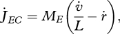
Figure 1 presents an overview of the various processes that are delineated by the standard DEB model. In our description of the various processes below, we assume that temperature is constant. In the standard DEB model, all rates depend on temperature in the same way to avoid that conversion efficiencies (from food to reserve, structure, offspring, products) become temperature-dependent; multiple-reserve systems are more flexible in this respect.

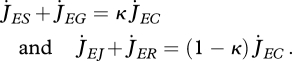
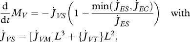
(a). Reserve dynamics drives metabolism

The core of DEB theory is that metabolism is fuelled by the mobilization of reserve during all life stages (embryo, juvenile and adult); reserve being replenished by assimilation after the maturity threshold for birth has been passed,

2.1

with for embryos (they do not feed), i.e. maturity M_H < M_H^b. This not only explains why embryos can grow (i.e. increase structure) without feeding, but also why starving individuals can for some time survive and pay maintenance costs without dying (Sousa et al. 2008).

The flux of mobilized reserve equals the sum of all metabolic activities, excluding feeding (and assimilation)

2.2

i.e. somatic (S) and maturity maintenance (J), maturation (or reproduction, R) and growth (G).

In combination with the constraint that mobilization only depends on the amounts of reserve and structure, weak homeostasis implies that the mobilization rate is (see Sousa et al. 2008)

2.3

where specific growth rate and structural length L can vary (equation 2.10), but energy conductance is constant. The residence time of ‘molecules’ in the reserve is , so the energy conductance for a fully grown individual ( at L = L_∞) equals . This relationship provides a simple interpretation of energy conductance as a parameter. The independence of the reserve dynamics of food availability provides the individual with some protection against environmental fluctuations and some control over its own metabolism; typically varies wildly, but always varies slowly.

With the combination of equations 2.1 and 2.3 and the definition of surface-specific maximum assimilation rate , the dynamics of the reserve density m_E = M_E /M_V amounts to:

2.4

which is independent of the specific growth rate . If assimilation is at the maximum then the reserve density m_E goes to a maximum value. This

2.5

is independent of the organism body size; only the embryo can exceed this maximum, because it obtained its reserve from the mother.

It turns out to be convenient to introduce the scaled reserve density e = m_E/m_Em; this dimensionless quantity varies between 0 and 1.

(b). Feeding and assimilation

Embryos do not feed; only juveniles and adults. Feeding only depends on substrate (food) density and amount of structure, not partaking in the other metabolic interactions. The heat increment of feeding suggests that there are processes associated with food processing only, i.e. that food goes through a set of chemical reactions that transform it into reserves (Sousa et al. 2008). This is the assimilation process that is characterized by a yield coefficient y_EX of reserve on food that is assumed to be constant (for a given type of food) owing to the strong homeostasis assumption.

Food uptake at food density X is linked to assimilation as

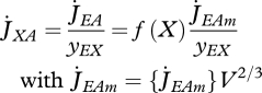2.6

where the scaled functional response f(X) = X/(X+K) is a monotonous increasing function of food density X with 0 ≤ f(X) ≤ 1, with half saturation constant , where is the maximum specific searching rate. The scaled functional response f results from the idea that the individual behaves as a synthesizing unit (SU; Kooijman 1998) with two sequential behavioural modes: searching and handling (including digestion and other metabolic work). Many extensions of this idea have been proposed. The original formulation of the behaviour SUs is stochastic but the standard DEB model only uses the mean feeding rate.

The maximum surface-specific assimilation rate is assumed to be constant, which is explained by the fact that digestion and other food processing activities depend on mass transport processes that occur through surfaces.

At constant food density, the reserve density evolves to (equation 2.5), which is independent of size and proportional to the scaled functional response. The scaled reserve density e = m_E /m_Em equals the scaled functional response f in equilibrium.

(c). Allocation

DEB's κ-rule for the allocation of mobilized reserve states that there is a constant fraction κ, with 0 ≤ κ ≤ 1, of mobilized reserve that is allocated to the soma (somatic maintenance and growth), i.e.

2.7

Somatic maintenance has priority over growth (i.e. increase in structure) and maturity maintenance has priority over maturation or reproduction. The ultimate size an individual can reach directly results from the competition between somatic maintenance and growth. Reproduction and growth do not compete directly with each other, which explains why they can occur simultaneously, as listed in the stylized empirical facts in table 2.

Static and dynamic generalizations of the κ-rule allow for the accurate description of the growth of body parts (including tumours), and the relationship with energetics. In particular fields, such as in fisheries research, it is standard to let growth directly compete with reproduction dynamically. This can be done by allowing κ to be a function of structure. The partitionability requirement for reserve dynamics (which is implied by weak homeostasis) allows this dependence (Kooijman 2000; Sousa et al. 2008). However, the dependence of κ on structure makes κ a design parameter implying that the maximum surface area specific assimilation rate can no longer be proportional to maximum length (Sousa et al. 2008). The consequence is that scaling relationships such as the interspecific Kleiber's Law would be lost as implied properties of the model. Moreover, if κ would depend on size, the von Bertalanffy growth curve no longer applies at constant food density. This empirical evidence together with the fact that the inverse von Bertalanffy growth rate increases linearly in the ultimate length (table 2) is strong support of the assumption that κ is generally constant.

(d). Somatic and maturity maintenance

The need to allocate energy to maintenance is intimately related with the second law of thermodynamics because the level of maturity, i.e. complexity of the organism, would decrease in the absence of energy spent on its maintenance.

Somatic maintenance is the use of reserve to fuel the set of processes that keep the organism alive, where and are the reserve flows allocated to volume, e.g. protein turnover, and to surface maintenance costs, e.g. heating in endotherms:

2.8

The volume-specific somatic maintenance costs are assumed to be constant; the turnover of structure comprises a big proportion of these costs, but they also include activity, for instance. The surface-specific somatic maintenance costs are only positive for particular taxa (endotherms and osmotic work for freshwater species). It is convenient to introduce the heating length 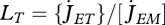. This turns out to be the reduction in ultimate length owing to surface-linked somatic maintenance.

Ultimate length L_∞ (when ) follows from the balance between assimilation and maintenance and does not depend on growth. Growth ceases if (cf. equation 2.7). Using equation 2.3 and 2.5, the result is L_∞ = fL_m − L_T with maximum length .

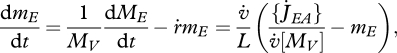
Reserve is assumed to require no maintenance, as empirically supported by the fact that freshly produced eggs almost exclusively consist of reserve and hardly respire (see Sousa et al. (2008) for a detailed explanation). Reserves do not need turnover; they have a limited residence time owing to assimilation and mobilization. In fully grown individuals, the residence time amounts to , but it is shorter in smaller individuals. This explains why babies need to feed more frequently than adults.

Maturity maintenance is the use of reserve to maintain the complexity of the structure where is the reserve flow allocated to this process and is the maturity maintenance rate coefficient:

2.9

The is constant in adults since for them maturity is constant, M_H = M_H^p.

(e). Growth

Growth is the increase of structure; the specific growth rate follows from the reserve dynamics (equation 2.3), the κ-rule (equation 2.7) and the somatic maintenance costs (equation 2.8). The result is

2.10

where is the mobilized reserve allocated to growth and y_VE is the yield of structure on reserve. Maximum length L_m, heating length L_T, investment ratio g are all given in table 7. Now the specific growth rate is specified, the mobilization rate in equation 2.3 is specified as well, so is the residence time t_E of ‘molecules’ in the reserve during ontogeny.

For any constant food level, the scaled reserve density e settles at the level of the scaled functional response e = f and the dynamics of structural length L = V^{1/3} = (M_V/[M_V])^1/3 simplifies to von Bertalanffy growth for juveniles and adults:

2.11

where the somatic maintenance rate coefficient is given in table 7. The inverse of the von Bertalanffy growth rate is thus linearly increasing with ultimate length, as listed in the stylized empirical facts in table 2.

If allocation of reserve to soma is not sufficient to pay the somatic maintenance costs, structure can shrink:

2.12

where the somatic maintenance costs , if paid from structure, have the same set-up as those paid from reserve (equation 2.8). A natural simplification is to assume that , but this ratio should be larger than one for thermodynamic reasons. Death by starvation occurs if structure, relative to the maximum the individual once had, decreases below a minimum. This minimum fraction is for supply systems typically smaller than for demand systems, but even for demand systems, empirical support for shrinking exists (Genoud 1988). Most species seem to avoid shrinking, e.g. by using the reproduction buffer to cover the somatic maintenance costs.

In extreme cases, species can sport suicide reproduction, and convert part of their structure to gametes before dying.

(f). Maturation and reproduction and initial state of the individual

Maturation is the use of reserve to increase the level of maturity, M_H. This level controls qualitative changes in metabolism (life-stage events). The initiation of feeding occurs at birth when M_H = M_H^b. The initiation of allocation to reproduction occurs at puberty when M_H = M_H^p; it is coupled to the ceasing of maturation. Other life-history events, such as cell division, metamorphosis or other stage transitions (e.g. to the pupal stage) occur also at threshold values for M_H.

Multicellular organisms typically have three life stages: embryo, juvenile, adult. At the start of development, age a is set to zero, structure M_V and maturity M_H are zero, M_V⁰ = 0 and M_H⁰ = 0, and the initial amount of reserve M_E⁰ is such that the reserve density m_E at birth equals that of the mother at egg formation; the maternal effect as listed in the stylized empirical facts in table 2. This fully specifies M_E⁰; for an efficient algorithm to obtain M_E⁰, see Kooijman (2009). Dividing unicellulars are treated as juveniles; division of maturity follows that of structure and division occurs if maturation exceeds a threshold.

The allocation to maturity (in embryos and juveniles) or reproduction (in adults) is

2.13

The change in maturity (in embryos and juveniles) is given by

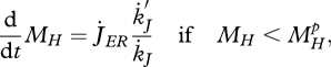2.14

where if , but for shrinking maturity (rejuvenation), it is a free constant parameter. Empirical evidence for rejuvenation induced by starvation is presented in Thomas & Ikeda (1987). The hazard rate owing to starvation is proportional to the difference between the maximum maturity level that the individual has reached and the actual level.

The reproduction buffer fills at rate for M_H = M_H^p. The details of the conversion of the reproduction buffer of females to a number of eggs are rather species-specific, typically including requirements on temperature and filling of the buffer; the conversion of the reproduction buffer of males to sperm is typically linked to female reproductive behaviour. The simplest buffer handling rule is to produce an egg as soon as the reproduction buffer allows; this rule involves no new parameters. The conversion of the content of the reproduction buffer to one or more eggs involves an overhead cost of the reproduction process, i.e. a fraction (1 − κ_R) of the converted buffer (and so of the reserve allocated to reproduction ) dissipates, and a fraction κ_R is fixed into eggs. The cost per egg equals the initial amount of reserve M_E⁰.

The reproduction rate in terms of numbers of eggs per time, is a delta function of time. Ignoring the effect of the reproduction buffer, and treating reproduction as a continuous process, the reproduction rate would amount to .

Foetal development is a variation on egg production, where the mother does not fill a reproduction buffer, but directly adds to the reserve of the foetus, bypassing its digestive system. This process can, therefore, not be seen as a feeding process from the foetal perspective.

(g). Three organizing fluxes in metabolism

An implication of strong homeostasis is that the different types of aggregated chemical reactions occurring in the organism have constant stoichiometries. These reactions are assimilation (), growth () and dissipation (), where dissipation is defined as:

2.15

and κ_R = 0 for the embryo and juvenile stages. Thus, metabolic transformation has three degrees of freedom; the flow of any compound (e.g. dioxygen), produced or consumed, in the organism is a weighted sum of these three organizing flows. The method of indirect calorimetry (table 3) is a particular case: the flow of heat is a weighted average of the fluxes of carbon dioxide, dioxygen and nitrogenous waste. Since, reserve is key to the ability to delineate these three fluxes (without reserve we would have two), the empirical success of the method of indirect calorimetry gives strong support to the topology of the standard DEB model.

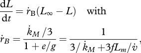
(h). Ageing

The hazard rate , i.e. the probability of dying, owing to ageing, is taken to be proportional to the density of damage compounds (e.g. modified proteins):

2.16

where is the dilution by growth and the change in ageing acceleration, which is proportional to the density of damage-inducing compounds (e.g. changed mitochondrial DNA). Damage compounds are generated by damage-inducing compounds at a rate proportional to the metabolic activity measured by the reserve mobilization rate (equation 2.3). The production of damage-inducing compounds is again taken to be proportional to the reserve mobilization rate (as quantifier for the respiration rate, excluding contributions from assimilation, which are supposed to have local effects only).

The change in ageing acceleration is given by

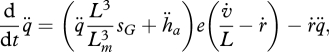2.17

where is the dilution by growth and the factor 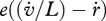is proportional to the mobilization rate; cf. equation 2.3. The proportionality factor 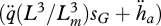increases linearly with because damage-inducing compounds promote their own production. This expression involves two new parameters, the Weibull ageing acceleration and the Gompertz stress coefficient s_G. The latter parameter is close to zero for most ectotherms, but for endotherms it is typically positive. It can be shown that if the growth period is short relative to the life span, both the Weibull and the Gompertz ageing models result, table 4. For further details on ageing see van Leeuwen et al. (2010).

(i). Parameters

Each individual is characterized in DEB theory by a set of primary parameters: the surface-area specific searching rate (feeding) , the surface-area specific maximum assimilation rate (assimilation) , the yield of reserve on food (digestion) y_EX and of structure on reserve (growth) y_VE, the energy conductance (mobilization of reserve) , surface and volume-specific somatic maintenance costs and , the specific maturity maintenance , the fraction of mobilized reserve allocated to soma κ, the reproduction efficiency κ_R, the maturity threshold levels that trigger the onset of feeding and reproduction M_H^b and M_H^p, the Weibull ageing acceleration and the Gompertz stress coefficient sG. This amounts to 14 primary parameters including the two ageing parameters and excluding parameters for species-specific handling rules for the reproduction buffer. The details of death by starvation involve another four parameters; these can be avoided by letting the individual die upon shrinking or starvation-induced rejuvenation. One can argue about the status of the mass–volume coupler [M_V]; this parameter relates measurements with no impact on processes.

The standard DEB model is meant to be the simplest in the DEB family that still has all essential features, a canonical form. Many applications need extensions of various types; the specification of respiration, for instance, requires the elemental composition of various compounds (food, faeces, reserve, structure). We agree with Nisbet et al. (2010) that some other applications, such as in population and ecosystem dynamics, require simplifications.

Most applications allow setting κ_R = 1 and ; the latter equality implies that maturity density, M_H/M_V, remains constant and metabolic switches occur at fixed amounts of structure. This means that the maturity thresholds can be replaced by structure thresholds and maturity can be avoided as state variable. If reproduction occurs with one offspring at a time, the reproduction buffer can be avoided as state variable. If investment in heating (or osmosis) is small, we have and s_G = 0. Ageing is not always an important cause of death in field situations; the ageing acceleration and the hazard rate can be avoided as state variables under those conditions, and the two ageing parameters are lost. All simplifications together reduce the standard DEB model to two state variables (reserve and structure) and nine parameters, while it still covers a full specification of feeding, digestion, maintenance, development, growth and reproduction over the full life cycle of the individual. This amounts to 9/6 = 1.5 parameter per process; we think a remarkable simplicity. Typical applications involve only a subset of these parameters because they do not involve all processes.

(j). Covariation of parameter values

A rough estimation of DEB parameters for each species can be made with the scaling relationships, i.e., based only on the species maximum size and a reference species; the accuracy of this estimation increases with the similarity between the species. The design parameters are and , which scale with maximum length, and M_H^b and M_H^p, which scale with maximum volume. All the other primary parameters are independent of size, so also independent of the maximum size of a species. The body-size scaling relationships can also be used partially, making optimal use of all data at hand (Kooijman et al. 2008; Kooijman 2010) to detect species-specific deviations from the general trend.

These rules also determine how properties that can be written as functions of the primary parameters depend on maximum length. An example is the respiration rate (i.e. the use of dioxygen). It works out to be approximately proportional to weight to the power 3/4, both inter- and intraspecifically (see the list of stylized facts in table 2), but for very different reasons. The weight-specific respiration rate decreases intraspecifically because growth decreases (and so the contribution of overhead costs of growth to respiration); it decreases interspecifically in fully grown adults because reserve density increases with the maximum size of a species and somatic maintenance is only paid for structure. The explanation offered by DEB theory also allows to understand taxon-specific variations in the scaling of respiration, since quite a few parameters contribute to the result and evolutionary adaptations cause deviations of parameters from the pattern. Many alternative attempts to explain the scaling of respiration fail to distinguish between intra- and interspecific comparisons, probably owing to the similarity of the numerical behaviour.

Many scaling relationships work out differently for intra- and interspecific comparisons. Feeding scales with surface intraspecifically, but with volume interspecifically, while maximum reproduction increases with size intraspecifically but decreases with size interspecifically.

The remarkable prediction for life span is that it scales with length if the Gompertz stress coefficient is positive (as expected for endotherms), but hardly scales with length if it is zero (as expected for ectotherms), which is consistent with empirical data (table 2).

3. Current research topics in Dynamic Energy Budget Theory

(a). The sub-individual level

The links that DEB theory establishes between the sub- and supra-individual levels together with the high amount of throughput data becoming available at the sub-individual level have allowed the use, test and development of DEB models at this organization level (van Leeuwen et al. 2010; Pecquerie et al. 2010; Vinga et al. 2010).

Vinga et al. (2010) use DEB theory for a top-down approach to understand the dynamic behaviour of metabolites. The individual level controls the size of the reserve fluxes that are associated with assimilation, dissipation and growth: , and . These fluxes impose constraints on the rates of aggregated chemical reactions and on the overall amount of each aggregated chemical compound at the sub-individual level. Vinga et al. compare the DEB approach with biochemical systems theory (BST) in modelling in vivo data of lactic acid bacteria under various conditions. In contrast with DEB theory, BST is a bottom-up approach that models each chemical compound and each chemical reaction explicitly. The complementarity between the two approaches is important in bringing new insights to unsolved problems that link the sub-individual and the individual levels such as the mechanisms underlying gene expression or the mechanisms underlying ageing (van Leeuwen et al. 2010).

Pecquerie et al. (2010) develop DEB theory further to provide a framework for stable isotope dynamics. The fundamental processes of the standard DEB model—assimilation, dissipation and growth—are further detailed into their anabolic and catabolic transformations to account for the mass balance of stable isotopes. Isotope dynamics reveals features that remain hidden in aggregate mass dynamics such as the turnover rate of structure. This turnover process has a catabolic as well as an anabolic component. Since turnover has a substantial contribution to somatic maintenance, it is also of importance to energetics. This DEB module on isotope dynamics will allow for the correct interpretation of the increasing amount of data becoming available on isotope ratios contributing to the identification of trophic web structures, the reconstruction of individual life histories, and the tracking of the flow of elements through ecosystems.

van Leeuwen et al. (2010) review the DEB-based approaches to ageing and link them to current research at the molecular/cellular level. The authors link alternative ageing DEB-based modelling approaches with different cellular senescence processes. This is a first step towards a fundamental understanding of the link between mechanisms of cellular senescence and ageing, at the individual level.

(b). The individual level

The mass, energy and entropy description of all fluxes, provided by DEB theory, are most useful to study the internal concentration of specific compounds such as isotopes (Pecquerie et al. 2010), reactive oxygen species  (van Leeuwen et al. 2010) and toxins (Jager & Klok 2010; Ducrot et al. 2010) that affect the performance of organisms at the individual level. The mode of action of a compound is, in the context of DEB theory, defined by the parameters that are affected. When the internal concentration increases, more and more parameters become affected, but at a sufficiently low concentration only a single parameter is significantly affected, but the consequences might be complex, involving feeding, growth and reproduction. For example, an increase in the specific maintenance rate, , leads directly to a decrease in growth, and ultimately also to a smaller adult that reproduces less while the decrease in the efficiency of reproduction, κ_R, leads to a decrease in the rate of reproduction (Jager et al. 2004), but does not affect growth or feeding. Jager and Klok compare several DEB approaches for analysing the toxicity of copper in the earthworm Dendrobaena octaedra: the Kooijman–Metz formulation (Kooijman & Metz 1984; which has no reserve or maturity), the DEBtox approach (Kooijman & Bedaux 1996; which has no explicit maturity) and the DEB3 approach (Kooijman 2010). Results on mortality and growth rate for the DEBtox and the DEB3 approach were similar. Also, they compare DEB based and empirical approaches concluding that only the former allow extrapolation for field relevant conditions. Ducrot et al. use the DEBtox model to assess the toxicity data of diquat on the gastropod Lymnaea stagnalis, where they include data on embryo development, making full use of the life-cycle features of DEB theory in variable environments, which is crucial for environmental risk assessment.

(c). The population level

The step from the individual to the population level requires extra rules for the interaction between individuals and for the transport of resources in the environment. The simplest interaction rule for the standard DEB model is that individuals only interact via competition for resources. The standard bookkeeping technique to follow the performance of populations as collections of individuals is (hyperbolic) partial differential equations (PDEs). Diekmann & Metz (2010) present a wider mathematical framework that removes some of the shortcomings of PDEs in this context. The standard DEB model has some features, however, that still cause mathematical problems including the existence of metabolic events (birth, puberty) that lead to singularities in the equations, the fact that eggs are not infinitesimally small and last but not least, DEB is deterministic (apart from the survival module). Some of these problems can be removed. For example, SU-dynamics (which is used to specify feeding) is stochastic by nature and differences between individuals can be implemented using different parameter values.

Other problems, however, are rather fundamental and call for individual-based approaches or a fully stochastic framework. For example, when feeding on a single resource in homogeneous space, the DEB rules imply that small (young) individuals can rather easily outcompete the large (old) individuals, perhaps to an extent that is not very realistic. There are several DEB solutions to this problem. Kearney et al. (2010) consider that food quality required by the individual depends on size. Large individuals mainly have to cover their maintenance cost (reproduction is low at the carrying capacity, where competition is strongest) while small individuals need to grow. Energy for maintenance can be supplied by carbohydrates and lipids while energy for growth must be supplied by a protein-rich resource. This set-up favours the large (old) individuals. Nisbet et al. (2010) consider survival to be maturity-dependent; in juveniles, the probability of dying is much more dependent on the food level, which favours adults. With this feature they have been able to understand the occurrence of daphnid population oscillations under particular conditions, using a reduced version of the DEB individual dynamics. They beautifully illustrate that not all details are important under all conditions; if food density is rather constant and different food levels are not compared, reserve and maturity typically play a minor role.

The step from the individual to the population levels can be done using a variety of schemes. Jager & Klok (2010) use DEB-structured individuals in matrix and continuous Euler–Lotka population models to extrapolate toxic effects from individuals to populations.  Kooi & van der Meer (2010) use a physiological-structured population to model the dynamics of a population in a semi-chemostat environment where reproduction is a discrete event process. In the case of organisms that reproduce by division, the transition from the individual to the population is simpler, because organisms can be considered as V1-morphs, i.e. individuals that change in shape during growth such that their surface area is proportional to volume. In this case, a population of a few big individuals behaves identically to that of many small ones if the sum of their masses match: the individual level completely drops out of the equations. This is the case in Lorena et al. (2010) and Poggiale et al. (2010), where population performance hence directly links to sub-individual physiology.

(d). Variable environments

Since DEB theory specifies the interaction between the individual and its environment dynamically, it has no problems at all with variable environments. This volume has a nice collection of examples, where these variations are explicitly used to study the underlying organization. Ducrot et al. (2010) use this feature when analysing the effects of a weed control agent when the concentrations vary in time; they show how DEB-based models can capture observed survival patterns where typical models fail.  Lorena et al. (2010) model microalgae populations in a chemostat with a variable light regime and study how the biochemical composition of microalgae depends on light. More specifically they discuss the relationship between chlorophyll, biomass and the production of exopolimeric substances; these are key features in the interpretation of remote sensing data.  Pecquerie et al. (2010) evaluate how variations in isotope concentrations in the environment work out for the organism. They do not make the common assumption that isotope dynamics is at equilibrium, and include the full metabolism in their analysis. Troost et al. (2010) adjust DEB individual models for cockles and mussels to a specific site by adjusting the functional response. With this model they detected food preferences in cockles and mussels, inferring the importance of detritus and intraspecific competition under field situations.

Kearney et al. (2010) position DEB theory in a wider ecological setting, linking it to the theories of biophysical ecology and the Geometric Framework for Nutrition. The combination of these fields stimulates the development of models at their interfaces that can shed more light on the detailed interaction of organisms and their environment. Biophysical ecology provides a framework for the climatic niche of an organism (distribution limits as constrained by heat and water balances) making use of spatial environmental data while the Geometric Framework for Nutrition provides a way to determine the nutritional niche of an organism (distribution limits as constrained by dietary needs) making use of information on the availability of food. These theories presently make use of allometrically derived static mass and energy budgets. By using DEB theory, these theories can model physiological rates across the life cycle under variable food and climatic environments and establish links between individuals and their functional traits and population. This is an essential step towards the goal of building predictive niche models that can tackle questions such as the impact of climate change on a species distribution.

(e). SUs: combining multiple mass and energy flows

The kinetics of SUs (Kooijman 1998, 2010) is an essential building block for the dynamics of multiple reserve and/or multiple structure organisms. SUs can be conceived as generalized enzymes that link the product fluxes to the arrival fluxes of substrate at the enzyme. Poggiale et al. (2010) interpret the different types of co-limitation in an SU context and demonstrate that these different types are of importance at the ecosystem level. Lorena et al. (2010) use SU-dynamics to model the co-limitation of photosynthesis by light and carbon dioxide and the co-limitation of growth by a carbon and nitrogen reserves. While Kearney et al. (2010) use SU-dynamics to transform food into separate nutrient reserve pools, and then regulate the assignment of reserves mobilized from each pool into maintenance, structure, maturity maintenance and reproductive output.

(f). Parameters

The generality of DEB theory allows the use of more parsimonious models (fewer parameters) to accurately describe experimental data under different environmental conditions. The DEB model for glycolysis in Lactococcus lactis uses much less parameters than a comparable BST model Vinga et al. (2010), while it better catches the differences between growth under aerobic and anaerobic conditions.

DEB rate parameters depend on temperature. Freitas et al. (2010) compare the temperature tolerance (this is the set of temperatures for which the Arrhenius relationship applies) and temperature sensitivity for a variety of marine species. Their results suggest that the width of the temperature tolerance range increases with the optimal growth temperature. Differences in life-history strategies of related species translated nicely in differences in parameter values: high-optimal growth temperatures, large tolerance ranges and high sensitivities are linked to low-specific assimilation rates and low-specific maintenance costs.

Although DEB theory does not use any optimization argument, it remains thought-provoking to study to what extent parameter values, or life-history traits, are optimal, or at least could be seen as the outcome of an evolutionary optimization process. The theory of adaptive dynamics is ideal for this, because there is no need to specify any explicit optimization criterion. Moreover, it includes the interactions between organisms and their environment and the long-term consequences of changes in traits in a natural way; the outcome depends on the realism of the ecosystem model. Kooi & van der Meer (2010) study the handling rules of the reproduction buffer of Macoma under seasonal forcing. They successfully capture the observed spawning behaviour of this iteroparous species, which spawns once a year; although, they were not able to correctly predict the timing of spawning. Application of adaptive dynamics with seasonal forcing is an impressive tour de force; more research is required to understand why Macoma spawns in spring. Moreover, Kooi & van der Meer (2010) demonstrate that the techniques that they use are a special case of bifurcation theory (Troost et al. 2007), which can lead to cross-fertilization.

Although a lot has been done already, the development of DEB theory has only started. Almost all contributions in this volume illustrate this in different ways. Future developments should include extensions in the sub-individual level, e.g. at the molecular level, and in the supra-individual level, e.g. the development of DEB-based biogeochemical climate models (Kooijman 2004). There are also open issues at the individual level such as the development of behavioural extensions, the formalization of multiple reserve and multiple structure organisms and DEB models for plants. The behavioural timescale including food searching, food selection, sleeping, social interaction, parental care, etc., is particularly important for animals and humans. Quite a few behavioural extensions have already been proposed using SU-dynamics but they have to be explored more systematically. Also, DEB models for plants have been proposed (Kooijman 2010), but they need to be tested against data; which has not been easy because detailed studies in plant biology are not available.

4. Concluding remarks

Given the richness of biodiversity on Earth, general explanatory models have to be lean, capturing taxon-specific phenomena in modules that extend the non-taxon-specific core. For particular applications (e.g. in ecosystem dynamics), the standard DEB model will be too complex, for other applications (e.g. in medicine and molecular biology) not detailed enough. This directly relates to the timescales of interest. Simplifications as well as extensions should be done, respecting a natural order in timescales, where the standard DEB model deals only with the slowest processes at the individual level. It makes little sense to include very fast processes if slower processes are not included. Extensions should be consistent with the existing assumptions.

Balancing realism at a detailed level against simplicity (in terms of numbers of parameters and variables) depends on subjective judgement and context. Although the standard DEB model is simple relative to the complexity of biological reality, estimating its parameters on the basis of published data is a challenge. Extensions make this problem worse, not easier, and we believe that obtaining accurate estimates for the primary parameters should generally have priority over extensions. We made a systematic start in the add_my_pet program (http://www.bio.vu.nl/thb/deb/deblab) and hope that the collection extends rapidly and improves in quality. We hope that a new generation of scientists will collect data in the light of DEB theory that allows the accurate estimation of its parameters and further critical testing of the underlying assumptions.

References

- Beer W. N., Anderson J. J.1997Modelling the growth of salmonid embryos. J. Theor. Biol. 189, 297–306 (doi:10.1006/jtbi.1997.0515) [DOI] [PubMed] [Google Scholar]
- Best J.1995The influence on intracellular enzymatic properties for kinetics data obtained from living cells. Cell. Comp. Physiol. 46, 1–27 (doi:10.1002/jcp.1030460102) [DOI] [PubMed] [Google Scholar]
- Blackman F. F.1905Optima and limiting factors. Ann. Bot. 19, 281–295 [Google Scholar]
- Bucher T. L.1983Parrot eggs, embryos, and nestlings—patterns and energetics of growth and development. Physiol. Zool. 56, 465–483 [Google Scholar]
- Chappell M. A., Bachman G. C., Hammond K. A.1997The heat increment of feeding in house wren chicks: magnitude, duration, and substitution for thermostatic costs. J. Comp. Physiol. B 167, 313–318 (doi:10.1007/s003600050079) [Google Scholar]
- Chen Y., Jackson D. A., Harvey H. H.1992A comparison of von Bertalanffy and polynomial functions in modeling fish growth data. Can. J. Fish. Aquat. Sci. 49, 1228–1235 (doi:10.1139/f92-138) [Google Scholar]
- Chen Y., Ke C. H., Zhou S. Q., Li F. X.2005Effects of food availability on feeding and growth of cultivated juvenile Babylonia formosae habei (Altena and Gittenberger 1981). Aquaculture Res. 36, 94–99 (doi:10.1111/j.1365-2109.2004.01189.x) [Google Scholar]
- Chilliard Y., Delavaud C., Bonnet M.2005Leptin expression in ruminants: nutritional and physiological regulations in relation with energy metabolism. Domest. Anim. Endocrinol. 29, 3–22 (doi:10.1016/j.domaniend.2005.02.026) [DOI] [PubMed] [Google Scholar]
- Clarke A., Johnston N. M.1999Scaling of metabolic rate with body mass and temperature in teleost fish. J. Anim. Ecol. 68, 893–905 (doi:10.1046/j.1365-2656.1999.00337.x) [DOI] [PubMed] [Google Scholar]
- Diekmann O., Metz J. A. J.2010How to lift a model for individual behaviour to the population level? Phil. Trans. R. Soc. B 365, 3523–3530 (doi:10.1098/rstb.2010.0100) [DOI] [PMC free article] [PubMed] [Google Scholar]
- Dou S., Masuda R., Tanaka M., Tsukamoto K.2002Feeding resumption, morphological changes and mortality during starvation in Japanese flounder larvae. J. Fish Biol. 60, 1363–1380 (doi:10.1111/j.1095-8649.2002.tb02432.x) [Google Scholar]
- Droop M. R.1973Some thoughts on nutrient limitation in algae. J. Phycol. 9, 264–272 [Google Scholar]
- Droop M. R.1974The nutrient status of algal cells in continuous culture. J. Mar. Biol. Assoc. UK 54, 825–855 (doi:10.1017/S002531540005760X) [Google Scholar]
- Droop M. R.198325 years of algal growth kinetics. Bot. Mar. 26, 99–112 (doi:10.1515/botm.1983.26.3.99) [Google Scholar]
- Du S. B., Mai K. S.2004Effects of starvation on energy reserves in young juveniles of abalone Haliotis discus hannai Ino. J. Shellfish Res. 23, 1037–1039 [Google Scholar]
- Ducrot V., Péry A. R. R., Lagadic L.2010Modelling effects of diquat under realistic exposure patterns in genetically differentiated populations of the gastropod Lymnaea stagnalis. Phil. Trans. R. Soc. B 365, 3485–3494 (doi:10.1098/rstb.2010.0047) [DOI] [PMC free article] [PubMed] [Google Scholar]
- Emerson S.1950The growth phase in neurospora corresponding to the logarithmic phase in unicellular organisms. J. Bacteriol. 60, 221–223 [DOI] [PMC free article] [PubMed] [Google Scholar]
- Ferreira B. P., Russ G. R.1994Age validation and estimation of growth-rate of the coral trout, Plectropomus leopardus, (Lacepede 1802) from Lizard Island, Northern Great Barrier Reef. Fish. Bull. 92, 46–57 [Google Scholar]
- Finch C. E.1990Longevity, senescence, and the genome. Chicago, IL: University of Chicago Press [Google Scholar]
- Fink P., Peters L., Von Elert E.2006Stoichiometric mismatch between littoral invertebrates and their periphyton food. Arch. Hydrobiol. 165, 145–165 (doi:10.1127/0003-9136/2006/0165-0145) [Google Scholar]
- Fisher R. A., Tippitt L. H. C.1928Limiting forms of the frequency distribution of the largest or the smallest member of a sample. Proc. Camb. Phil. Soc. 24, 180–190 (doi:10.1017/S0305004100015681) [Google Scholar]
- Frazer N. B., Gibbons J. W., Greener J. L.1990Exploring Fabens growth interval model with data on a long-lived vertebrate, Trachemys scripta (Reptilia: Testudinata). Copeia 1, 112–118 (doi:10.2307/1445827) [Google Scholar]
- Freitas V., Cardoso J. F. M. F., Lika K., Peck M. A., Campos J., Kooijman S. A. L. M, van der Veer H. W.2010Temperature tolerance and energetics: a dynamic energy budget-based comparison of North Atlantic marine species. Phil. Trans. R. Soc. B 365, 3553–3565 (doi:10.1098/rstb.2010.0049) [DOI] [PMC free article] [PubMed] [Google Scholar]
- Gallardo C. S., Manque C., Filun M.2004Comparative resistance to starvation among early juveniles of some marine muricoidean snails. Nautilus 118, 121–126 [Google Scholar]
- Galluci V. F., Quinn T. J.1979Reparameterizing, fitting, and testing a simple growth-model. Trans. Am. Fish. Soc. 108, 14–25 (doi:10.1577/1548-8659(1979)108<14:RFATAS>2.0.CO;2) [Google Scholar]
- Genoud M.1988Energetic strategies of shrews: ecological constraints and evolutionary implications. Mammal. Rev. 4, 173–193 (doi:10.1111/j.1365-2907.1988.tb00083.x) [Google Scholar]
- Gompertz B.1825On the nature of the function expressive of the law of mortality, and on a new method of determining the value of life contingencies. Phil. Trans. R. Soc. 27, 513–585 (doi:10.1098/rstl.1825.0026) [Google Scholar]
- Hanegraaf P. P. F., Stouthamer A. H., Kooijman S. A. L. M.2000A mathematical model for yeast respiro-fermentative physiology. Yeast 16, 423–437 (doi:10.1002/(SICI)1097-0061(20000330)16:5<423::AID-YEA541>3.0.CO;2-I) [DOI] [PubMed] [Google Scholar]
- Hawkins P. A. J., Butler P. J., Woakes A. J., Gabrielsen G. W.1997Heat increment of feeding in Brunnich's guillemot Uria lomvia. J. Exp. Biol. 200, 1757–1763 [DOI] [PubMed] [Google Scholar]
- Heino M., Kaitala V.1999Evolution of resource allocation between growth and reproduction in animals with indeterminate growth. J. Evol. Biol. 12, 423–429 (doi:10.1046/j.1420-9101.1999.00044.x) [Google Scholar]
- Hill H. V.1910The possible effects of aggregation on the molecules of haemoglobin on its dissociation curves. J. Physiol. 40, pIV–VII. [Google Scholar]
- Hirche H. J., Kattner G.1993Egg production and lipid content of Calanus glacialis in spring: indication of a food-dependent and food-independent reproductive mode. Mar. Biol. 117, 615–622 (doi:10.1007/BF00349773) [Google Scholar]
- Holling C. S.1959Some characteristics of simple types of predation and parasitism. Can. Entomol. 91, 385–398 (doi:10.4039/Ent91385-7) [Google Scholar]
- Hubert M. F., Laroque P., Gillet J. P., Keenan K. P.2000The effects of diet, ad libitum feeding, and moderate and severe dietary restriction on body weight, survival, clinical pathology parameters, and cause of death in control Sprague Dawley rats. Toxicol. Sci. 58, 195–207 (doi:10.1093/toxsci/58.1.195) [DOI] [PubMed] [Google Scholar]
- Huggett A. S., Widdas W. F.1951The relationship between mammalian foetal weight and conception age. J. Physiol. 114, 306–317 [DOI] [PMC free article] [PubMed] [Google Scholar]
- Hungate R. E.1975The rumen microbial ecosystem. Ann. Rev. Ecol. Syst. 6, 39–66 (doi:10.1146/annurev.es.06.110175.000351) [Google Scholar]
- Huxley J. S.1932Problems of relative growth. London, UK: Methuen Co [Google Scholar]
- Ingenbleek Y.2006The nutritional relationship linking sulfur to nitrogen in living organisms. J. Nutr. 136, 1641–1651 [DOI] [PubMed] [Google Scholar]
- Jager T., Klok C.2010Extrapolating toxic effects on individuals to the population level: the role of dynamic energy budgets. Phil. Trans. R. Soc. B 365, 3531–3540 (doi:10.1098/rstb.2010.0137) [DOI] [PMC free article] [PubMed] [Google Scholar]
- Jager T., Crommentuijn T., van Gestel C. A. M., Kooijman S. A. L. M.2004Simultaneous modelling of multiple endpoints in life-cycle toxicity tests. Environ. Sci. Technol. 38, 2894–2900 (doi:10.1021/es0352348) [DOI] [PubMed] [Google Scholar]
- Janes D. N., Chappell M. A.1995The effect of ration size and body-size on specific dynamic action in adelie penguin chicks, Pygoscelis-adeliae. Physiol. Zool. 68, 1029–1044 [Google Scholar]
- Jorgensen C., Fiksen O.2006State-dependent energy allocation in cod (Gadus morhua). Can. J. Fish. Aquat. Sci. 63, 186–199 (doi:10.1139/f05-209) [Google Scholar]
- Kearney M., Simpson S. J., Raubenheimer D., Helmuth B.2010Modelling the ecological niche from functional traits. Phil. Trans. R. Soc. B 365, 3469–3483 (doi:10.1098/rstb.2010.0034) [DOI] [PMC free article] [PubMed] [Google Scholar]
- Kirk K. L.1997Life-history responses to variable environments: starvation and reproduction in planktonic rotifers. Ecology 78, 434–441 (doi:10.1890/0012-9658(1997)078[0434:LHRTVE]2.0.CO;2) [Google Scholar]
- Kjesbu O. S., Klungsoyr J., Kryvi H., Witthames P. R., Walker M. G.1991Fecundity, atresia, and egg size of captive atlantic cod (Gadus morhua) in relation to proximate body-composition. Can. J. Fish. Aquat. Sci. 48, 2333–2343 (doi:10.1139/f91-274) [Google Scholar]
- Kleiber M.1932Body size and metabolism. Hilgardia 6, 315–353 [Google Scholar]
- Kooi B. W., van der Meer J.2010Bifurcation theory, adaptive dynamics and dynamic energy budget-structured populations of iteroparous species. Phil. Trans. R. Soc. B 365, 3579–3590 (doi:10.1098/rstb.2010.0173) [DOI] [PMC free article] [PubMed] [Google Scholar]
- Kooijman S. A. L. M.1998The synthesizing unit as model for the stoichiometric fusion and branching of metabolic fluxes. Biophys. Chem. 73, 179–188 (doi:10.1016/S0301-4622(98)00162-8) [DOI] [PubMed] [Google Scholar]
- Kooijman S. A. L. M.2000Dynamic energy and mass budgets in biological systems. Cambridge, UK: Cambridge University Press [Google Scholar]
- Kooijman S. A. L. M.2001Quantitative aspects of metabolic organization: a discussion of concepts. Phil. Trans. R. Soc. Lond. B 356, 331–349 (doi:10.1098/rstb.2000.0771) [DOI] [PMC free article] [PubMed] [Google Scholar]
- Kooijman S. A. L. M.2004On the coevolution of life and its environment. In Scientists debate Gaia: the next century (eds Schneider S. H., Miller J. R., Crist E., Boston P. J.), ch. 30, pp. 343–351 Cambridge, MA: MIT Press [Google Scholar]
- Kooijman S. A. L. M.2009What the egg can tell about its hen: embryo development on the basis of dynamic energy budgets. J. Math. Biol. 58, 377–394 (doi:10.1007/s00285-008-0195-x) [DOI] [PubMed] [Google Scholar]
- Kooijman S. A. L. M.2010Dynamic energy budget theory for metabolic organization. Cambridge, UK: Cambridge University Press [Google Scholar]
- Kooijman S. A. L. M., Bedaux J. J. M.1996Analysis of toxicity tests on daphnia survival and reproduction. Water Res. 30, 1711–1723 (doi:10.1016/0043-1354(96)00054-1) [Google Scholar]
- Kooijman S. A. L. M., Hengeveld R.2005The symbiontic nature of metabolic evolution. In Current themes in theoretical biology: a Dutch perspective (eds Reydon T. A. C., Hemerik L.), pp. 159–202. Dordrecht, The Netherlands: Springer [Google Scholar]
- Kooijman S. A. L. M., Metz J. A. J.1984On the dynamics of chemically stressed populations: the deduction of population consequences from effects on individuals. Ecotoxicol. Environ. Saf. 8, 254–274 (doi:10.1016/0147-6513(84)90029-0) [DOI] [PubMed] [Google Scholar]
- Kooijman S. A. L. M., Segel L. A.2005How growth affects the fate of cellular substrates. Bull. Math. Biol. 67, 57–77 (doi:10.1016/j.bulm.2004.06.003) [DOI] [PubMed] [Google Scholar]
- Kooijman S. A. L. M., Troost T. A.2007Quantitative steps in the evolution of metabolic organisation as specified by the dynamic energy budget theory. Biol. Rev. 82, 1–30 (doi:10.1111/j.1469-185X.2006.00006.x) [DOI] [PubMed] [Google Scholar]
- Kooijman S. A. L. M., Auger P., Poggiale J. C., Kooi B. W.2003Quantitative steps in symbiogenesis and the evolution of homeostasis. Biol. Rev. 78, 435–463 (doi:10.1017/S1464793102006127) [DOI] [PubMed] [Google Scholar]
- Kooijman S. A. L. M., Sousa T., Pecquerie L., van der Meer J., Jager T.2008From food-dependent statistics to metabolic parameters, a practical guide to the use of dynamic energy budget theory. Biol. Rev. 83, 533–552 [DOI] [PubMed] [Google Scholar]
- Kozlowski J.1996Optimal allocation of resources explains interspecific life-history patterns in animals with indeterminate growth. Proc. R. Soc. Lond. B 263, 559–566 (doi:10.1098/rspb.1996.0084) [Google Scholar]
- Krol E., Redman P., Thomson P. J., Williams R., Mayer C., Mercer J. G., Speakman J. R.2005Effect of photoperiod on body mass, food intake and body composition in the field vole, Microtus agrestis. J. Exp. Biol. 208, 571–584 (doi:10.1242/jeb.01429) [DOI] [PubMed] [Google Scholar]
- Kunji E. R. S., Ubbink T., Matin A., Poolman B., Konings W. N.1993Physiological responses of Lactococcus lactis ML3 to alternating conditions of growth and starvation. Arch. Microbiol. 159, 372–379 (doi:10.1007/BF00290920) [Google Scholar]
- Letcher B. H., Rice J. A., Crowder L. B., Binkowski F. P.1996Size-dependent effects of continuous and intermittent feeding on starvation time and mass loss in starving yellow perch larvae and juveniles. Trans. Am. Fish. Soc. 125, 14–26 (doi:10.1577/1548-8659(1996)125<0014:SDEOCA>2.3.CO;2) [Google Scholar]
- Leudeking R., Piret E. L.1959A kinetic study of the lactic acid fermentation. J. Biochem. Microbiol. Technol. Eng. 1, 393 (doi:10.1002/jbmte.390010406) [Google Scholar]
- Lorena A., Marques G. M., Kooijman S. A. L. M., Sousa T.2010Stylized facts in microalgal growth: interpretation in a dynamic energy budget context. Phil. Trans. R. Soc. B 365, 3509–3521 (doi:10.1098/rstb.2010.0101) [DOI] [PMC free article] [PubMed] [Google Scholar]
- Marr A. G., Nilson E. H., Clark D. J.1963The maintenance requirement of Escherichia coli. Ann. NY Acad. Sci. 102, 536–548 (doi:10.1111/j.1749-6632.1963.tb13659.x) [Google Scholar]
- Mayneord W. V.1932On a law of growth of jensen's rat sarcoma. Am. J. Cancer 16, 841–846 [Google Scholar]
- Molnar T., Szabo A., Szabo G., Szabo C., Hancz C.2006Effect of different dietary fat content and fat type on the growth and body composition of intensively reared pikeperch Sander lucioperca (L.). Aquaculture Nutr. 12, 173–182 (doi:10.1111/j.1365-2095.2006.00398.x) [Google Scholar]
- Monod J.1942Recherches sur la croissance des cultures bacteriennes, 2nd edn. Paris, France: Hermann [Google Scholar]
- Morowitz H. J.1968Energy flow in biology. New York, NY: Academic Press [Google Scholar]
- Nespolo R. F., Castaneda L. E., Roff D. A.2005The effect of fasting on activity and resting metabolism in the sand cricket, Gryllus firmus: a multivariate approach. J. Insect Physiol. 51, 61–66 (doi:10.1016/j.jinsphys.2004.11.005) [DOI] [PubMed] [Google Scholar]
- Nisbet R. M., McCauley E., Johnson L. R.2010Dynamic energy budget theory and population ecology: lessons from Daphnia. Phil. Trans. R. Soc. B 365, 3541–3552 (doi:10.1098/rstb.2010.0167) [DOI] [PMC free article] [PubMed] [Google Scholar]
- Nisbet R., Muller E., Lika K., Kooijman S. A. L. M.2000From molecules to ecosystems through dynamic energy budget models. J. Anim. Ecol. 69, 913–926 (doi:10.1046/j.1365-2656.2000.00448.x) [Google Scholar]
- Pearl R.1927The growth of populations. Q. Rev. Biol. 2, 532–548 (doi:10.1086/394288) [Google Scholar]
- Pecquerie L., Nisbet R. M., Fablet R., Lorrain A., Kooijman S. A. L. M.2010The impact of metabolism on stable isotope dynamics: a theoretical framework. Phil. Trans. R. Soc. B 365, 3455–3468 (doi:10.1098/rstb.2010.0097) [DOI] [PMC free article] [PubMed] [Google Scholar]
- Peters R. H.1983The ecological implications of body size. Cambridge, UK: Cambridge University Press [Google Scholar]
- Pettit T. N.1982Embryonic oxygen-consumption and growth of Laysan and black-footed albatross. Am. J. Physiol. Regul. Integr. Comp. Physiol. 242, 121–128 [DOI] [PubMed] [Google Scholar]
- Pirt S. J.1965The maintenance energy of bacteria in growing cultures. Proc. R. Soc. Lond. B 163, 224–231 (doi:10.1098/rspb.1965.0069) [DOI] [PubMed] [Google Scholar]
- Poggiale J.-C., Baklouti M., Queguiner B., Kooijman S. A. L. M.2010How far details are important in ecosystem modelling: the case of multi-limiting nutrients in phytoplankton–zooplankton interactions. Phil. Trans. R. Soc. B 365, 3495–3507 (doi:10.1098/rstb.2010.0165) [DOI] [PMC free article] [PubMed] [Google Scholar]
- Putter A.1920Studies on the physiological similarity. VI. Similarities in growth. Pflugers Archiv für die Gesamte Physiologie des Menschen und der Tiere 180, 280 [Google Scholar]
- Rahn H., Ar A.1974The avian egg: incubation time and water loss. Condor 76, 147–152 (doi:10.2307/1366724) [Google Scholar]
- Richman S.1958The transformation of energy by Daphnia pulex. Ecol. Monogr. 76, 273 (doi:10.2307/1942243) [Google Scholar]
- Ricklefs R. E., Finch C. E.1995Aging: a natural history. New York, NY: Scientific American Library [Google Scholar]
- Roberts R. D., Lapworth C., Barker R. J.2001Effect of starvation on the growth and survival of post-larval abalone (Haliotis iris). Aquaculture 200, 323–338 (doi:10.1016/S0044-8486(01)00531-2) [Google Scholar]
- Romijn C., Lokhorst W.1951Foetal respiration in the hen—the respiratory metabolism of the embryo. Physiol. Comp. Oecolog. 2, 187–197 [Google Scholar]
- Rosen D. A. S., Trites A. W.1997Heat increment of feeding in Steller sea lions, Eumetopias jubatus. Comp. Biochem. Physiol. A-Mol. Integr. Physiol. 118, 877–881 (doi:10.1016/S0300-9629(97)00039-X) [DOI] [PubMed] [Google Scholar]
- Ross J. L., Stevens T. M., Vaughan D. S.1995Age, growth, mortality, and reproductive biology of red drums in North Carolina waters. Trans. Am. Fish. Soc. 124, 37–54 (doi:10.1577/1548-8659(1995)124<0037:AGMARB>2.3.CO;2) [Google Scholar]
- Russell N. R., Wootton R. J.1992Appetite and growth compensation in the European minnow, Phoxinus phoxinus (Cyprinidae), following short periods of food restriction. Environ. Biol. Fishes 34, 277–285 (doi:10.1007/BF00004774) [Google Scholar]
- Savage V. M., Gillooly J. F., Woodruff W. H., West G. B., Allen A. P., Enquist B. J., Brown J. H.2004The predominance of quarter-power scaling in biology. Funct. Ecol. 57, 257–282 (doi:10.1111/j.0269-8463.2004.00856.x) [Google Scholar]
- Schwartz C. C., Hundertmark K. J.1993Reproductive characteristics of Alaskan moose. J. Wildl. Manage. 57, 454–468 (doi:10.2307/3809270) [Google Scholar]
- Seale J. L., Rumpler W. V., Moe P. W.1991Description of a direct-indirect room-sized calorimeter. Am. J. Physiol. Endocrinol. Metab. 57, E306–E320 [DOI] [PubMed] [Google Scholar]
- Shine R., Iverson J. B.1995Patterns of survival, growth and maturation in turtles. Oikos 72, 343–348 (doi:10.2307/3546119) [Google Scholar]
- Smith S.1957Early development and hatching. In The physiology of fishes, vol. 1 (ed. Brown M. E.), pp. 323–359 San Diego, CA: Academic Press [Google Scholar]
- Sousa T., Mota R., Domingos T., Kooijman S. A. L. M.2006Thermodynamics of organisms in the context of dynamic energy budget theory. Phys. Rev. E 74, 051901. (doi:10.1103/PhysRevE.74.051901) [DOI] [PubMed] [Google Scholar]
- Sousa T., Domingos T., Kooijman S. A. L. M.2008From empirical patterns to theory: a formal metabolic theory of life. Phil. Trans. R. Soc. B 363, 2453–2464 (doi:10.1098/rstb.2007.2230) [DOI] [PMC free article] [PubMed] [Google Scholar]
- Steenbergen R., Nanowski T. S., Nelson R., Young S. G., Vance J. E.2006Phospholipid homeostasis in phosphatidylserine synthase-2-deficient mice. Biochim. Biophys. Acta Mol. Cell Biol. Lipids 1761, 313–323 [DOI] [PubMed] [Google Scholar]
- Stockhoff B. A.1991Starvation resistance of gipsy moth, Lymantria dispar (L.) (Lepidoptera: Lymantriidae): tradeoffs among growth, body size and survival. Oecologia 82, 422–429 (doi:10.1007/BF00317588) [DOI] [PubMed] [Google Scholar]
- Stromgren T., Cary C.1984Growth in length of Mytilus edulis L. fed on different algal diets. J. Exp. Mar. Biol. Ecol. 76, 23–34 (doi:10.1016/0022-0981(84)90014-5) [Google Scholar]
- Strum S. C.1991Weight and age in wild olive baboons. Am. J. Primatol. 25, 219–237 (doi:10.1002/ajp.1350250403) [DOI] [PubMed] [Google Scholar]
- Summers W. C.1971Age and growth of Loligo pealei, a population study of the common Atlantic coast squid. Biol. Bull. (Woods Hole) 141, 189–201 (doi:10.2307/1540003) [Google Scholar]
- Thomas P. G., Ikeda T.1987Sexual regression, shrinkage, re-maturation and growth of spent female Euphausia superba in the laboratory. Mar. Biol. 95, 357–363 (doi:10.1007/BF00409565) [Google Scholar]
- Thornton W. M.1917The relation of oxygen to the heat of combustion of organic compounds. Phil. Mag. 33, 196–203 [Google Scholar]
- Troost T. A., Kooi B. W., Kooijman S. A. L. M.2005When do mixotrophs specialize? Adaptive dynamics theory applied to a dynamic energy budget model. Math. Biosci. 193, 159–182 (doi:10.1016/j.mbs.2004.06.010) [DOI] [PubMed] [Google Scholar]
- Troost T. A., Kooi B. W., Kooijman S. A. L. M.2007Bifurcation analysis can unify ecological and evolutionary aspects of ecosystems. Ecol. Mod. 204, 253–268 (doi:10.1016/j.ecolmodel.2007.01.007) [Google Scholar]
- Troost T. A., Wijsman J. W. M., Saraiva S., Freitas V.2010Modelling shellfish growth with dynamic energy budget models: an application for cockles and mussels in the Oosterschelde (southwest Netherlands). Phil. Trans. R. Soc. B 365, 3567–3577 (doi:10.1098/rstb.2010.0074) [DOI] [PMC free article] [PubMed] [Google Scholar]
- van Leeuwen I. M. M., Vera J., Wolkenhauer O.2010Dynamic energy budget approaches for modelling organismal ageing. Phil. Trans. R. Soc. B 365, 3443–3454 (doi:10.1098/rstb.2010.0071) [DOI] [PMC free article] [PubMed] [Google Scholar]
- Vinga S., Neves A. R., Santos H., Brandt B. W., Kooijman S. A. L. M.2010Subcellular metabolic organization in the context of dynamic energy budget and biochemical systems theories. Phil. Trans. R. Soc. B 365, 3429–3442 (doi:10.1098/rstb.2010.0156) [DOI] [PMC free article] [PubMed] [Google Scholar]
- von Bertalanffy L.1938A quantitative theory of organic growth (Inquiries on growth laws. II.). Hum. Biol. 10, 181–213 [Google Scholar]
- Weibull W.1951A statistical distribution of wide applicability. J. Appl. Mech. 18, 293–297 [Google Scholar]
- Weindruch R., Walford R. L., Fligiel S., Guthrie D.1986The retardation of aging in mice by dietary restriction: longevity, cancer, immunity and lifetime energy intake. J. Nutr. 116, 641–654 [DOI] [PubMed] [Google Scholar]
- Whitehead P. J. P.1987Respiration of Crocodylus johnstoni embryos. In Wildlife management: crocodiles and alligators (eds Webb G. J. W., Manolis S. C., Whitehead P. J. P.). Sydney, Australia: University of Minnesota Press [Google Scholar]
- Zheng H. P., Ke C. H., Zhou S. Q., Li F. X.2005Effects of starvation on larval growth, survival and metamorphosis of ivory shell Babylonia formosae habei Altena et al., 1981 (Neogastropoda: Buccinidae). Aquaculture 243, 357–366 (doi:10.1016/j.aquaculture.2004.10.010) [Google Scholar]
- Zonneveld C., Kooijman S. A. L. M.1993Comparative kinetics of embryo development. Bull. Math. Biol. 55, 609–635 [DOI] [PubMed] [Google Scholar]