

Abstract
We studied a prey–predator system in which both species evolve. We discuss here the conditions that result in coevolution towards a stable equilibrium or towards oscillations. First, we show that a stable equilibrium or population oscillations with small amplitude is likely to occur if the prey's (host's) defence is effective when compared with the predator's (parasite's) attacking ability at equilibrium, whereas large-amplitude oscillations are likely if the predator's (parasite's) attacking ability exceeds the prey's (host's) defensive ability. Second, a stable equilibrium is more likely if the prey's defensive trait evolves faster than the predator's attack trait, whereas population oscillations are likely if the predator's trait evolves faster than that of the prey. Third, when the adaptation rates of both species are similar, the amplitude of the fluctuations in their abundances is small when the adaptation rate is either very slow or very fast, but at an intermediate rate of adaptation the fluctuations have a large amplitude. We also show the case in which the prey's abundance and trait fluctuate greatly, while those of the predator remain almost unchanged. Our results predict that populations and traits in host–parasite systems are more likely than those in prey–predator systems to show large-amplitude oscillations.
Keywords: coevolution, population cycles, stability, adaptive dynamics, speed of evolution
1. Introduction
Coevolution in species with antagonistic interactions, such as in predator–prey, host–parasite or exploiter–victim systems, is considered one of the most important processes creating and maintaining species diversity on Earth. In spite of research efforts by both empiricists and theoreticians in evolutionary biology, demonstrating coevolution in nature is still difficult. Recently, coevolutionary dynamics have been revealed by experimental studies with micro-organisms (Buckling & Rainey 2002; Forde et al. 2004, 2007; Buckling et al. 2006; Lopez-Pascua & Buckling 2008), and coevolution has also been confirmed to occur in field studies (Berenbaum & Zangerl 1992; Benkman et al. 2001; Bergelson et al. 2001; Brodie et al. 2002; Soler et al. 2003; Toju & Sota 2006; Hoso et al. 2007).
Since population sizes in a predator–prey system have an inherent tendency to oscillate, one research focus has been to ascertain under what conditions coevolution of prey and predator leads to population stability or oscillation. Experimental studies have shown that the evolution of traits is sufficiently rapid to influence the population dynamics (Hairston et al. 1999, 2005; Shertzer et al. 2002; Yoshida et al. 2003; Agashe 2009). If the ecological dynamics and evolutionary dynamics occur on similar time scales, they should be considered within the same framework (e.g. Abrams & Matsuda 1997).
Many theoretical studies have addressed coevolution in a predator–prey system (see Abrams 2000). Most of these studies have assumed a bidirectional axis of prey vulnerability (Abrams 2000), in which prey can reduce their risk by having a defensive trait value either larger or smaller than that of the most vulnerable phenotype, which is determined by the predator's phenotype (Brown & Vincent 1992; Marrow et al. 1992, 1996; Marrow & Cannings 1993; Dieckmann et al. 1995; Van der Laan & Hogeweg 1995; Dieckmann & Law 1996; Abrams & Matsuda 1997; Doebeli 1997; Gavrilets 1997; Khibnik & Kondrashov 1997; Nuismer et al. 2005; Weitz et al. 2005; Dercole et al. 2006). This model is appropriate, for example, if the focal trait is body size and the predator feeds most efficiently on prey within a limited size range. In contrast, only a few theoretical studies have assumed a unidirectional axis of prey vulnerability in which the traits are the defensive or attack skills of the two species: a higher predator ability increases the capture rate, and a higher prey ability reduces it (Saloniemi 1993; Frank 1994; Abrams & Matsuda 1997; Sasaki & Godfray 1999; Nuismer et al. 2007). This model is appropriate for trait interactions between predator and prey such as speed versus speed, toxin versus antitoxin and weapon versus armour. Both bidirectional and unidirectional predation situations occur widely in nature (Nuismer et al. 2007).
In this paper, we study the coevolutionary dynamics of a predator–prey system with a unidirectional axis of prey vulnerability: the predator's trait v is the effectiveness of its attacks, and the prey's trait u is the effectiveness of its defence. We examine the conditions for coevolution to result in a stable equilibrium or large-amplitude oscillations. We focus on how constraints on the two species with regard to attack or defence adaptation affect the likelihood of evolutionary oscillation or evolutionary stability. We also examine how the speed of evolutionary adaptation in the two species influences the population dynamics. For the ecological dynamics we adopt the Lotka–Volterra (LV) system as the simplest model, and for the evolutionary dynamics we adopt a quantitative genetic model (Iwasa et al. 1991) in which the evolution of the prey's trait u and the predator's trait v is controlled by quantitative genetic dynamics. The speed of change of these traits is determined by their additive genetic variance and the generation time.
From the results of mathematical analyses, we predict the following coevolutionary consequences. First, population size and trait equilibria tend to be stable if the prey's defence is effective against the predator's attacking ability, whereas the population and trait dynamics tend to show cycles if the predator's attacking ability exceeds the prey's defence ability. Second, population size and trait equilibria are more likely to be stable if the prey evolves faster than the predator, whereas population and trait cycles are likely if the predator evolves faster than the prey. Third, when the speed of evolutionary adaptation of the two species is similar, the magnitude of population size fluctuations is small when the adaptation rate is either very slow or very fast, but large when the adaptation rate is intermediate. We also find the case in which the prey's population size and trait value fluctuate greatly, while the predator's trait value and population size remain almost unchanged. We then discuss the implications of our results with regard to the coevolutionary dynamics of parasites and pathogens, as well as those of predators and prey, the life–dinner principle of asymmetry in predator–prey relationships (Dawkins & Krebs 1979), and the cryptic dynamics concept (Yoshida et al. 2007).
2. Model
(a). Dynamics of population size
We consider the following simple Lotka–Volterra population dynamics model of predator and prey,
| 2.1a |
| 2.1b |
where X and Y are prey and predator densities, respectively; r is the per capita prey growth rate; a is the capture rate (i.e. the rate at which the predator captures its prey); g is the conversion efficiency, which relates the predator's birth rate to prey consumption; and d is the death rate of the predator.
Parameters r, a and g are functions of certain traits of the two species. We assume that a is a function of the predator trait v and the prey trait u: that is, a(u, v); a decreases as the difference between u and v increases, which is an appropriate model for trait interactions such as speed–speed, weapon–armour and toxin–antitoxin (Saloniemi 1993; Frank 1994; Abrams & Matsuda 1997; Sasaki & Godfray 1999; Gavrilets et al. 2001; Nuismer et al. 2007). Specifically, a is the sigmoidal function, 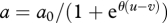 , where a0 is the maximum capture rate and θ is the shape parameter of the function. As θ increases, the function approaches a step function. If the value of the prey's trait u is much greater than that of the predator's trait v, the prey can escape predation effectively, and a is very small. In contrast, if the values of the predator's trait v is much greater than that of the prey's trait u, then the capture rate a is large.
The cost of developing the trait in each species is modelled by assuming that r and g are decreasing functions of u and v, respectively (trade-off functions). The rates of decrease (−r′ and −g′) indicate the strength of the cost constraint on the prey and the predator, respectively.
(b). Dynamics of evolutionary adaptation
We model the evolutionary dynamics of the population mean trait values, u and v, by a quantitative trait evolution model (Iwasa et al. 1991) as follows (see electronic supplementary material, appendix A):
| 2.2a |
| 2.2b |
where  and
and  represent the speed of evolutionary adaptation, which is equal to the additive genetic variance divided by the generation time, in the prey and the predator, respectively. We call this parameter the adaptation speed. For simplicity, we assume that the speed is constant. WX and WY are prey fitness and predator fitness, respectively, defined as the per capita rate of population growth: WX = r(u) − a(u − v)Y and WY = g(v)a(u − v)X − d. WX is a function of trait
  of the focal prey individual and WY is a function of trait
  . They also depend on the population mean traits u and v (Iwasa et al. 1991). Equation (2.2) indicates that the rate of adaptive change in the traits should be proportional to the selection gradient. If the selection gradient is positive (negative), selection pushes the population towards higher (lower) trait values. At evolutionary equilibrium, equation (2.2) becomes zero.
A formula similar to equation (2.2) has also been adopted to describe habitat choice, behavioural change, learning and phenotypic plasticity, by which individuals can shift the value of their trait in a direction that will improve the expected fitness (Abrams et al. 1993). Here, the dynamics expressed by equation (2.2) indicate adaptive change in traits by either genetic evolution or an individual's shifting of its phenotype. In the following discussion, we consider both to be ‘adaptation’ in the broad sense.
The four differential equations (2.1a), (2.1b), (2.2a) and (2.2b) describe the coupled coevolutionary and ecological dynamics of a prey and a predator species, which we analyse further below.
3. Results
In figure 1, we show the coevolutionary dynamics of population sizes (X and Y) and traits (u and v) for several different values of the speed of evolutionary adaptation  , which was chosen to be the same in both species. In this example, cyclic oscillation occurs, but depending on conditions, the dynamics may converge to equilibrium. We first discuss the condition for a stable or unstable equilibrium. Then, we discuss how the speed of adaptation affects the dynamic behaviour of the population sizes and traits of the two species.
Figure 1.

An example of non-equilibrium dynamics in relation to the speed of adaptation. We adopted the linear functions r = r0(1−ρXu) and g = g0(1−ρY v), where r0 and g0 are the basal per capita prey growth rate and the basal conversion efficiency of the predator, respectively, and ρX and ρY represent the strength of the trade-off in the prey and the predator, respectively. We assumed that  . The solid and dotted lines indicate the dynamics of the prey and predator, respectively. The inset in the lower panel of (a) enlarges a portion of panel. The parameter values are ρX = ρY = 2, r0 = 1, g0 = 1, a0 = 3, θ = 20 and d = 0.3. The initial values are (X, Y, u, v) = (1, 0.5, 0.1, 0.1).
(a). Conditions leading to equilibria or cycles
To ascertain the conditions leading to coevolutionary cycles, we analyse the local stability of a non-trivial equilibrium in the coevolutionary system described by equations (2.1) and (2.2) (the results are explained in the electronic supplementary material, appendix B).
Figure 2 illustrates the parameter regions in which the equilibrium is stable (white) and unstable (shaded). In the shaded, unstable regions, the system oscillates perpetually. The two cases shown in figure 2 differ with regard to the strength of the constraints on the two species.
Figure 2.

The parameter regions in which the equilibrium is stable or unstable. The two axes are  and
and  . We adopted the linear functions r = r0(1−ρXu) and g = g0(1−ρYv). The white and shaded regions indicate the parameter ranges in which the equilibrium is stable and unstable, respectively. (a) u* = v*. We assumed ρX = ρY=2. (b) u* < v*. The shaded region is the unstable region when ρX = 1.98 and ρY = 2. The ordered pairs show (ρX, ρY), corresponding to each boundary (dotted lines) between stable and unstable regions, with the region on the left side of the boundary unstable and the one on the right stable. The other parameter values are r0 = 1, g0 = 1, a0 = 3, θ = 20 and d = 0.2.
If the constraint on the prey's adaptation is greater than that on the predator's adaptation, the value of the prey's defensive trait is smaller than the value of the predator's attacking trait at equilibrium (u* ≤ v*). The asterisks denote the trait values at equilibrium. Figure 2a illustrates the case where u* = v*, but the result where u* < v* is very similar. In this case, in a large fraction of the parameter space the equilibrium is unstable. In contrast, when the constraint on the prey's defence trait is weaker than that on the predator's attacking trait, the value of the prey's defence trait is greater than the value of the predator's trait (u* > v*; figure 2b). In this case, in a large fraction of the parameter space a stable equilibrium exists. The contrast between figure 2a and b illustrates that the equilibrium is more likely to be stable if u* > v* than if u* ≤ v*. Examination of many numerical results similar to those shown in figure 2 supports this conclusion.
Moreover, the results shown in figure 2b also suggest that the equilibrium tends to be stable when  , implying that if the speed of evolutionary adaptation of the prey is faster than that of the predator, then the dynamics tend to be stable. If the adaptation reflects genetic evolution (rather than phenotypic plasticity or behavioural choice), the speed of adaptation is the additive genetic variance of the focal trait (Iwasa et al. 1991) divided by the mean generation time. Hence, if the generation time of the prey is shorter than that of the predator, then the system is likely to converge to an evolutionary equilibrium.
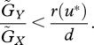
In cases of extreme parameter values, we can further analyse local stability. For example, when evolutionary adaptation is very fast ( ), we can show that the equilibrium is locally stable if the following inequality holds:
| 3.1 |
and, moreover, that the equilibrium is unstable if equation (3.1) is reversed. The derivation is explained in the electronic supplementary material, appendix C. This result implies that very fast evolution leads to stability if the equilibrium trait value of the prey is larger than that of the predator. In other words, if the constraint on the prey's trait is weaker than that on the predator's, the equilibrium is likely to be stable.
In the case that evolution is very slow ( ), and if the trade-off functions r(u) and g(v) are linear, the stability condition is again very simple (see the electronic supplementary material, appendix D). When u* > v*, the system is always locally stable if
 |
3.2 |
Also, we can show that if the trade-off functions are linear, the equilibrium is always locally stable when coevolution is slow and u* = v* (figure 2a). If  , this equilibrium is globally stable: numerical analysis shows that starting from any initial condition, the system converges to equilibrium. In contrast, if
  , the equilibrium is only locally stable, and if the initial state is far from the equilibrium, the system converges to a periodic oscillation with a moderately large amplitude. This limit cycle is also locally stable.
Although the example illustrated in figure 2 assumes linear trade-off functions, we also numerically examined the local stability of the equilibrium in the case of nonlinear trade-off functions and obtained results that were qualitatively the same as those for linear trade-off functions. The parameter region in which the equilibrium is stable becomes broader when r″(u*), g″(v*) < 0 than the case with a linear trade-off (r″(u*), g″(v*) = 0; see electronic supplementary material, figs S1 and S2), but becomes narrower when r″(u*), g″(v*) > 0 than the case with a linear trade-off such that the entire region of  space is locally unstable (the double primes indicate the second derivative of the function). In other words, if the cost of developing a trait increases at a decelerating rate as the trait value increases, coevolutionary cycles are likely to occur (Abrams & Matsuda 1997).
In summary, if the prey's defensive trait is less constrained and if the prey's speed of adaptation is faster when compared with the predator's attack trait and speed of adaptation, then the dynamics are likely to converge to an evolutionary equilibrium. In the opposite situation, the system is more likely to evolve to show oscillations.
(b). Speed of adaptation and the amplitude of oscillation
Next, we examine how the speed of adaptation influences the behaviour of the system. To show this, we focus on the case in which the speeds of adaptation of the two species are equal ( ).
).
We observe two different patterns of dependence of the dynamics on the speed of adaptation (figures 3 and 4). In both cases, as the speed of adaptation  increases, the amplitude of the population cycles changes in a non-monotonic manner. The amplitude of the population oscillation is small when the speed of evolution is very slow or very fast, but large when the speed is intermediate. In contrast, the amplitude of the trait cycles shows two patterns: either the amplitudes increase as the speed of adaptation increases (figure 3), or they reach a peak when the speed of adaptation is intermediate and then abruptly stabilize above a threshold speed (figure 4). These differences are closely related to the behaviour of the system when
  is large (see our discussion of equation (3.1)). If u* > v*, the second pattern is more likely to occur, but if u* < v*, the first pattern is more likely.
Figure 3.

Bifurcation diagrams of (a,b) population and (c) trait dynamics, and (d) the ratio of the amplitudes of oscillation in the two species in relation to the speed of adaptation. The points indicate the minimum and maximum values. The black and grey points in panel (c) are the maximum and minimum trait values in the prey and predator, respectively. The Arabic numerals in square brackets above the panels indicate three phases: [1] trait–abundance cycle; [2] resonance; and [3] trait–trait cycle phases (see text). Other parameter values are ρX = ρY = 1, r0 = 1, g0 = 1, a0 = 6, θ = 40 and d = 0.45. The initial values are (X, Y, u, v) = (1, 0.5, 0.1, 0.1).
Figure 4.

Bifurcation diagrams of (a,b) population and (c) trait dynamics, and (d) the ratio of the amplitudes of oscillation in the two species in relation to the speed of adaptation. The Arabic numerals in square brackets above the panels indicate phases, as in figure 3; [4] indicates the stationary phase (see text). Parameters are the same as in figure 2 except for ρX = 1 and ρY = 1.01.
As we increase  from a very small value to a very large one, we can recognize several distinct phases as described below (figures 3 and 4).
(i). Trait–abundance cycle phase
When the speed of evolutionary adaptation is slow, the sizes of the two populations oscillate. The amplitude and the period of the oscillation do not change much with variations in the speed of adaptation  . For very small
  , the equilibrium is locally stable (see figure 2a, near the origin). But the system also has a stable limit cycle with a fixed amplitude. The fixed amplitudes of these limit cycles with small
  are shown in figures 3 and 4.
Note that the amplitudes of the oscillations of both the trait value and the population size of the prey are much larger than those of the predator (figures 3d and 4d). This result indicates that the prey's population size and trait value oscillate with a moderately large amplitude, whereas the predator's population size and trait value remain almost stationary in this phase. The ratio of the magnitude of oscillation in X to that in Y and the ratio of the oscillation in u to that in v are both much greater than 1 (figures 3d and 4d). This asymmetric pattern can be explained by considering the between-species difference in the sensitivity of trait dynamics to the population dynamics (electronic supplementary material, appendix E). We call this parameter region the ‘trait–abundance cycle’ phase, because the trait and the abundance of the prey both fluctuate although no clear oscillation occurs in the predator's trait or abundance.
(ii). Resonance phase
When the speed of adaptation  exceeds a threshold value, the amplitude of the oscillation of the population sizes of both species suddenly becomes large. The traits of both species also begin to fluctuate with large amplitude (figures 3a,b and 4a,b). In the Lotka–Volterra model, which does not incorporate adaptation of the species, the system shows an inherent tendency towards oscillation, and the coevolutionary dynamics of the two species are coupled with the population dynamics, causing large-amplitude oscillations. This phenomenon is comparable to a resonance between the population dynamics and the evolutionary dynamics; hence, we call this phase the ‘resonance’ phase.
(iii). Trait–trait cycle phase
When the speed of adaptation  is even faster, the amplitude of the population size fluctuation becomes smaller. In contrast, the trait dynamics shows oscillations of a larger amplitude (figures 3c and 4c). As the two species coevolve, their trait values show large-amplitude fluctuations, whereas the abundances of the two species either stabilize or oscillate with a rather small amplitude. We call this parameter region the ‘trait–trait cycle’ phase, because the traits of both species fluctuate with a large amplitude but the oscillation in the abundances is less conspicuous.
The amplitude of the population dynamics oscillations decreases as the speed of the evolutionary adaptation  increases. This may be explained intuitively as follows. In the Lotka–Volterra model, in which the trait values do not change adaptively (fixed u and v), the system can oscillate at many different frequencies: when the amplitude is small, the period of the oscillation is short, and when the amplitude is larger, the period is longer. The period of oscillation for the highest frequency is about 2π/√rd, as calculated from the eigenvalue at the central equilibrium. This shortest period, in the example of figure 1, is about 25.7 at equilibrium. When the adaptive dynamics are very fast, the period of oscillation becomes shorter than this value, resulting in a small amplitude of oscillation.
(iv). Stationary phase with fast adaptation
Only in the case of the second pattern of the dependence of the dynamics on the speed of adaptation, shown in figure 4, do we observe the complete cessation of oscillation in population sizes and trait values for very large  . This pattern is likely to occur when u* > v*. Note that the transition from phase [3], which exhibits a moderately large oscillation, to this phase of perfect equilibrium is quite sudden.
In our discussion thus far (figures 1, 3 and 4), we have assumed that the speed of evolutionary adaptation was the same in both species. We also examined the case in which the speed of evolution differed between the two species. If the speed of evolution of the prey increases while that of the predator remains fixed, the dynamics tend to become stabilized. In contrast, if the speed of evolution of the predator increases with that of the prey remaining fixed, the dynamics tend to be destabilized. If the speed of evolutionary adaptation is not very different between the two species, however, the dynamics are similar to those illustrated in figures 1, 3 and 4.
The patterns shown in figures 3 and 4 were determined by assuming linear trade-off functions, but the patterns are qualitatively the same even if we adopt nonlinear trade-off functions.
(c). The effect of prey's density dependence
To examine the robustness of these results, we also studied numerically the cases with prey's density dependence: we assumed that the prey's population size follows logistic growth, r(1 − X/K), in the absence of the predator.
First we found that the strength of density dependence largely influences the stability: very weak density dependence (small K) tends to stabilize the system (electronic supplementary material, fig. S3a). However, as shown in figure 2b, the tendency of the equilibrium to be stable when  remains valid for the case with density dependence (electronic supplementary material, fig. S3a). In addition, according to the result shown in figure 2a,b, that the equilibrium tends to be stable when u* > v* while it tends to be unstable when u* < v* is also valid with the density-dependent regulation of prey population (electronic supplementary material, fig. S3b). When evolutionary adaptation is very fast (
 ) or very slow (
 ), we can further analyse local stability (electronic supplementary material, appendix F). The analysis shows that the local stability conditions are very similar with and without density dependence when adaptation is very slow, and exactly the same when adaptation is very fast.
In this system, we also find an interesting pattern of the dynamics on the speed of adaptation shown in LV type (electronic supplementary material, fig. S4). Although there are some difference in the dynamics between the density dependence model (electronic supplementary material, fig. S4) and the LV type (figures 3 and 4), in both models we can recognize the ‘resonance’ phase when the speed of adaptation is medium, the ‘trait–trait cycle’ phase when the speed of adaptation is relatively fast and the ‘stationary phase’ when the speed of adaptation is very fast. However, we could not recognize the ‘trait–abundance cycle’ phase in the density dependence model, and instead we have the ‘stationary phase’ when the speed of adaptation is very slow. In short, most conclusions obtained for the LV model also hold in the presence of the density dependence of prey population growth.
3. Discussion
We analysed the coevolutionary dynamics of a predator–prey system with a unidirectional axis with regard to the prey's defence and the predator's attack abilities. We also examined the conditions under which the coevolution of predator and prey resulted in coevolutionary oscillation or in a stable equilibrium, and how the speed of evolutionary adaptation of the two species controls the population dynamics.
We demonstrated that the coevolutionary consequences strongly depend on the dominance of adaptation and the relative magnitudes of the speed of adaptation between the two species. Population sizes and trait values tend towards stable equilibrium if the prey's defence is effective when compared with the predator's attacking ability. Otherwise, the dynamics tend to show cycles. In addition, a stable equilibrium is more likely if the prey evolves faster than the predator.
We also found that the population dynamics and coevolutionary dynamics depend critically on the speed of evolutionary adaptation. The magnitude of fluctuation in the population size is relatively small when adaptation is very slow and it is even smaller when adaptation is very fast, whereas a large amplitude of fluctuation is associated with an intermediate speed of adaptation. As the speeds of evolutionary adaptation in the two species increase simultaneously, we observe several distinct phases: trait–abundance cycle, resonance, trait–trait cycle and stationary with fast adaptation phases.
(a). Host–parasite versus prey–predator systems
Taken together, these results suggest that a host–parasite system would tend to evolve towards instability with large-amplitude oscillations, because in such a system a single host tends to be attacked by a number of parasite species. Hence, evolutionary adaptation by the host is constrained with respect to defence against any particular parasite. In contrast, parasites tend to be more specific than hosts, and to achieve reproductive success they must succeed in breaking the host's defence. Hence, we expect the coevolutionary equilibrium generally to be parasite-dominated (u* < v*). Our results indicate that in this situation the equilibrium becomes more unstable. In addition, parasites tend to have a much smaller body size, and hence a shorter generation time, than the host. A second result of our analysis indicates that this difference in generation time also makes the coevolutionary outcome more unstable, because a shorter generation time causes the evolutionary adaptation of the parasites to be faster than that of the host.
In contrast, a predator–prey relationship may have a more stable coevolutionary outcome than a host–parasite relationship. Predators tend to have a larger body size than their prey, so they adapt more slowly than their prey. In addition, a generalist predator tends to be less adapted for attacking a particular prey species. This asymmetry has been discussed by Dawkins & Krebs (1979).
Previous theoretical studies have shown that host–parasite interactions are likely to be unstable (Frank 1994; Sasaki & Godfray 1999), and that predator–prey interactions are likely to be stable in a coevolutionary system (Saloniemi 1993; Abrams & Matsuda 1997). This contrast, though not clearly noted before, is supported by our results here.
An experimental study has shown that predator–prey dynamics are stabilized by evolution of the defence of the prey if the cost of that defence is small (Jones et al. 2009). The population dynamics are likely to be stabilized if the defence cost is small. This finding may be consistent with our result that a weaker constraint on adaptation by the prey than on adaptation by the predator is likely to stabilize the population dynamics at the evolutionary endpoint. We also showed that faster adaptation by the prey than by the predator is likely to stabilize the population dynamics. This result may explain the reported stabilizing effect of an inducible defence of the prey on predator–prey dynamics (Verschoor et al. 2004).
(b). Intermediate adaptation speed principle
An interesting finding of this study is that population abundances show much larger fluctuations when the speed of evolutionary adaptation is intermediate (the intermediate adaptation speed principle). This finding suggests that either a loss of genetic variance in populations with high evolutionary potential or an increase in genetic variance in populations with low evolutionary potential can cause destabilization of predator–prey dynamics. This result may be important in conservation practice.
The intermediate adaptation speed principle has been observed in other, more realistic predator–prey systems. For example, we tested the other model system that incorporated logistic growth of the prey population and type II functional response. All the model systems showed a dynamics pattern similar to that found in this study (Mougi & Iwasa, submitted).
(c). Fast adaptation
The adaptation speed critically influences the stability of predator–prey dynamics. The same equation used to describe evolution in our model can be regarded as a description of phenotypic plasticity, in which individuals shift their trait in the direction that improves their expected fitness (Abrams et al. 1993): that is, fast coevolutionary adaptation can be considered equivalent to reciprocal phenotypic plasticity. In reciprocal phenotypic plasticity, for example, a prey with an inducible defence and a predator with an inducible attack may interact antagonistically in a sort of arms race (Agrawal 2001; Kopp & Tollrian 2003; Kishida et al. 2006). Mougi & Kishida (2009) showed that reciprocal phenotypic plasticity can stabilize predator–prey dynamics when the defence is effective. This observation is consistent with the result reported in this paper that very fast adaptation can stabilize the dynamics, particularly when the value of the prey's trait is clearly larger than that of the predator's trait at equilibrium. Another finding of this paper is that the speed of adaptation can also strongly affect the stability, which is consistent with a previous result that fast adaptive foraging by predators can stabilize and maintain a complex food web (Kondoh 2003).
(d). Cryptic dynamics
The results of experiments with micro-organisms have recently shown that, when a prey species is rapidly evolving, the predator can exhibit large-amplitude cycles, while the prey's abundance remains nearly constant (Yoshida et al. 2007). This phenomenon is called ‘cryptic dynamics’. In the Lotka–Volterra coevolutionary system studied in this paper, cryptic dynamics were also observed to occur where the trait value and the abundance of the prey species showed a large-amplitude cycle while those of the predator remained nearly constant.
We also found an asymmetric relationship between population dynamics and evolutionary dynamics. The prey's trait and abundance cycles were much larger than those of the predator when adaptation was very slow. In contrast, in both species, the amplitude of the trait oscillation was large, and that of the population size oscillation was small, when adaptation was fast. We might call this result ‘cryptic red queen dynamics’.
(e). Evolution of genetic variance
In this paper, we focus on how the magnitude of speed of evolution (controlled by additive genetic variance and generation time) affects the population dynamics, assuming that the speed itself remains constant. Several previous studies have examined the cases in which the genetic variances in two interacting species evolve (Sasaki & Godfray 1999; Nuismer et al. 2005, 2007; Kopp & Gavrilets 2006). The models that assumed a bidirectional axis of prey vulnerability have predicted that genetic variation can be maintained at unequal levels: very small variation in the predator (parasite) species and relatively high variation in the prey (host) species (Nuismer et al. 2005; Kopp & Gavrilets 2006). This would be because the predator (parasite) tends to experience stabilizing selection and the prey (host) tends to experience disruptive selection. In contrast, the models that assumed a unidirectional axis of prey vulnerability have predicted that genetic variation can be maintained at almost equal levels (Sasaki & Godfray 1999; Nuismer et al. 2007). If this is also true in our model, the argument about the speed of evolutionary adaptation and stability may reduce to that about generation times and stability. The examination of whether any of the conclusions in this paper change when additive genetic variance also changes in evolution is an important theme of future theoretical study.
In the near future, our predictions will be testable empirically by manipulating the evolutionary potential of the two species or observing the relationship between generation times and population dynamics.
Acknowledgements
We are very grateful to K. Nishimura, K. Uriu and S. Wada for their valuable comments on this study. This study was supported by a Grant-in-Aid for a Research Fellow from the Japan Society for the Promotion of Science and a Research Fellowship for Young Scientists (no. 20*01655) to A.M. and by a Grant-in-Aid (B) to Y.I.
References
- Abrams P. A.2000The evolution of predator-prey interactions: theory and evidence. Annu. Rev. Ecol. Syst. 31, 79–105 (doi:10.1146/annurev.ecolsys.31.1.79) [Google Scholar]
- Abrams P. A., Matsuda H.1997Fitness minimization and dynamic instability as a consequence of predator–prey coevolution. Evol. Ecol. 11, 1–20 (doi:10.1023/A:1018445517101) [Google Scholar]
- Abrams P. A., Harada Y., Matsuda H.1993Unstable fitness maxima and stable fitness minima in the evolution of continuous traits. Evol. Ecol. 7, 465–487 (doi:10.1007/BF01237642) [Google Scholar]
- Agashe D.2009The stabilizing effect of intraspecific genetic variation on population dynamics in novel and ancestral habitats. Am. Nat. 174, 255–267 (doi:10.1086/600085) [DOI] [PubMed] [Google Scholar]
- Agrawal A. A.2001Phenotypic plasticity in the interactions and evolution of species. Science 294, 321–326 (doi:10.1126/science.1060701) [DOI] [PubMed] [Google Scholar]
- Benkman C. W., Holimon W. C., Smith J. W.2001The influence of a competitor on the geographic modaic of coevolution between crossbills and lodgepole pine. Evolution 55, 282–294 [DOI] [PubMed] [Google Scholar]
- Berenbaum M. R., Zangerl A. R.1992Genetics of physiological and behavioural resistance to host furanocoumarins in the parsnip webworm. Evolution 46, 1373–1384 (doi:10.2307/2409943) [DOI] [PubMed] [Google Scholar]
- Bergelson J., Dawyer G., Emerson J. J.2001Models and data on plant-enemy coevolution. Annu. Rev. Genet. 35, 469–499 (doi:10.1146/annurev.genet.35.102401.090954) [DOI] [PubMed] [Google Scholar]
- Brodie E. D., Jr, Ridenhour B. J., Brodie E. D., III2002The evolutionary response of predators to dangerous prey: hot spots and cold spots in the geographic mosaic of coevolution between garter snakes and newts. Evolution 56, 2067–2082 [DOI] [PubMed] [Google Scholar]
- Brown J. S., Vincent G. T. L.1992Organization of predator–prey communities as an evolutionary game. Evolution 46, 1269–1283 (doi:10.2307/2409936) [DOI] [PubMed] [Google Scholar]
- Buckling A., Rainey P. B.2002Antagonistic coevolution between a bacterium and a bacteriophage. Proc. R. Soc. Lond. B 269, 931–936 (doi:10.1098/rspb.2001.1945) [DOI] [PMC free article] [PubMed] [Google Scholar]
- Buckling A., Wei Y., Massey R. C., Brockhurst M. A., Hochberg M. E.2006Antagonistic coevolution with parasites increases the cost of host deleterious mutations. Proc. R. Soc. B 273, 45–49 (doi:10.1098/rspb.2005.3279) [DOI] [PMC free article] [PubMed] [Google Scholar]
- Dawkins R., Krebs J. R.1979Arms races between and within species. Proc. R. Soc. Lond. B 205, 489–511 (doi:10.1098/rspb.1979.0081) [DOI] [PubMed] [Google Scholar]
- Dercole F., Ferrière R., Gragnani A., Rinaldi S.2006Coevolution of slow–fast populations: evolutionary sliding, evolutionary pseudo-equilibria and complex Red Queen dynamics. Proc. R. Soc. B 273, 983–990 (doi:10.1098/rspb.2005.3398) [DOI] [PMC free article] [PubMed] [Google Scholar]
- Dieckmann U., Law R.1996The dynamical theory of coevolution: a derivation from stochastic ecological processes. J. Math. Biol. 34, 579–612 (doi:10.1007/BF02409751) [DOI] [PubMed] [Google Scholar]
- Dieckmann U., Maroow P., Law R.1995Evolutionary cycling in predator–prey interactions: population dynamics and the Red Queen. J. Theor. Biol. 176, 91–102 (doi:10.1006/jtbi.1995.0179) [DOI] [PubMed] [Google Scholar]
- Doebeli M.1997Genetic variation and the persistence of predator-prey interactions in the Nicholson–Bailey model. J. Theor. Biol. 188, 109–120 (doi:10.1006/jtbi.1997.0454) [Google Scholar]
- Forde S. E., Thompson J. N., Bohannan B. J. M.2004Adaptation varies through space and time in a coevolving host–parasitoid interaction. Nature 431, 841–844 (doi:10.1038/nature02906) [DOI] [PubMed] [Google Scholar]
- Forde S. E., Thompson J. N., Bohannan B. J. M.2007Gene flow reverses an adaptive cline in a coevolving host–parasitoid interaction. Am. Nat. 169, 794–801 (doi:10.1086/516848) [DOI] [PubMed] [Google Scholar]
- Frank S. A.1994Coevolutionary genetics of hosts and parasites with quantitative inheritance. Evol. Ecol. 8, 74–94 (doi:10.1007/BF01237668) [Google Scholar]
- Gavrilets S.1997Coevolutionary chase in exploiter–victim systems with polygenic characters. J. Theor. Biol. 186, 527–534 (doi:10.1006/jtbi.1997.0426) [DOI] [PubMed] [Google Scholar]
- Gavrilets S., Arnqvist G., Friberg U.2001The evolution of female mate choice by sexual conflict. Proc. R. Soc. B 268, 531–539 [DOI] [PMC free article] [PubMed] [Google Scholar]
- Hairston N. G., Jr, Lampert W., Cáceres C. E., Holtmeier C. L., Weider L. J., Gaedke M. U., Fischer J., Fox J. A., Post D. M.1999Rapid evolution revealed by dormant eggs. Nature 401, 446 (doi:10.1038/46731) [Google Scholar]
- Hairston N. G., Jr, Ellner S. P., Geber M. A., Yoshida T., Fox J. A.2005Rapid evolution and the convergence of ecological and evolutionary time. Ecol. Lett. 8, 1114–1127 (doi:10.1111/j.1461-0248.2005.00812.x) [Google Scholar]
- Hoso M., Asami T., Hori M.2007Right-handed snakes: convergent evolution of asymmetry for functional specialization. Biol. Lett. 3, 169–172 (doi:10.1098/rsbl.2006.0600) [DOI] [PMC free article] [PubMed] [Google Scholar]
- Iwasa Y., Pomiankowski A., Nee S.1991The evolution of costly mate preferences. II. The ‘handicap’ principle. Evolution 45, 1431–1442 (doi:10.2307/2409890) [DOI] [PubMed] [Google Scholar]
- Jones L. E., Becks L., Ellner S. P., Hairston N. G., Jr, Yoshida T., Fussmann G. F.2009Rapid contemporary evolution and clonal food web dynamics. Phil. Trans. R. Soc. B 364, 1571–1579 (doi:10.1098/rstb.2009.0004) [DOI] [PMC free article] [PubMed] [Google Scholar]
- Khibnik A. I., Kondrashov A. S.1997Three mechanisms of Red Queen dynamics. Proc. R. Soc. Lond. B 264, 1049–1056 (doi:10.1098/rspb.1997.0145) [Google Scholar]
- Kishida O., Mizuta Y., Nishimura K.2006Reciprocal phenotypic plasticity in a predator–prey interaction between larval amphibians. Ecology 87, 1599–1604 (doi:10.1890/0012-9658(2006)87[1599:RPPIAP]2.0.CO;2) [DOI] [PubMed] [Google Scholar]
- Kondoh M.2003Foraging adaptation and the relationship between food-web complexity and stability. Science 299, 1388–1391 (doi:10.1126/science.1079154) [DOI] [PubMed] [Google Scholar]
- Kopp M., Gavrilets S.2006Multilocus genetics and the coevolution of quantitative traits. Evolution 60, 1321–1336 [PubMed] [Google Scholar]
- Kopp M., Tollrian R.2003Reciprocal phenotypic plasticity in a predator–prey system: inducible offences against inducible defences? Ecol. Lett. 6, 742–748 (doi:10.1046/j.1461-0248.2003.00485.x) [Google Scholar]
- Lopez-Pascua L. D. C., Buckling A.2008Increasing productivity accelerates host–parasite co-evolution. J. Evol. Biol. 21, 853–860 [DOI] [PubMed] [Google Scholar]
- Marrow P., Cannings C.1993Evolutionary instability in predator-prey systems. J. Theor. Biol. 160, 135–150 (doi:10.1006/jtbi.1993.1008) [Google Scholar]
- Marrow P., Law R., Cannings C.1992The coevolution of predator–prey interactions: ESSs and Red Queen dynamics. Proc. R. Soc. Lond. B 250, 133–141 (doi:10.1098/rspb.1992.0141) [Google Scholar]
- Marrow P., Dieckmann U., Law R.1996Evolutionary dynamics of predator–prey systems: an ecological perspective. J. Math. Biol. 34, 556–578 (doi:10.1007/BF02409750) [DOI] [PubMed] [Google Scholar]
- Mougi A., Iwasa Y.Submitted Resonance, cryptic cycles, and phase differences in predator–prey adaptive dynamics. [Google Scholar]
- Mougi A., Kishida O.2009Reciprocal phenotypic plasticity can lead to stable predator–prey interaction. J. Anim. Ecol. 78, 1172–1181 (doi:10.1111/j.1365-2656.2009.01600.x) [DOI] [PubMed] [Google Scholar]
- Nuismer S. L., Doebeli M., Browning D.2005The coevolutionary dynamics of antagonistic interactions mediated by quantitative traits with evolving variances. Evolution 59, 2073–2082 [PubMed] [Google Scholar]
- Nuismer S. L., Ridenhour B. J., Oswald B.2007Antagonistic coevolution mediated by phenotypic differences between quantitative traits. Evolution 61, 1823–1834 (doi:10.1111/j.1558-5646.2007.00158.x) [DOI] [PubMed] [Google Scholar]
- Saloniemi I.1993A coevolutionary predator–prey model with quantitative characters. Am. Nat. 141, 880–896 (doi:10.1086/285514) [DOI] [PubMed] [Google Scholar]
- Sasaki A., Godfray H. C. J.1999A model for the coevolution of resistance and virulence in coupled host–parasitoid interactions. Proc. R. Soc. Lond. B 266, 455–463 (doi:10.1098/rspb.1999.0659) [Google Scholar]
- Shertzer K. W., Ellner S. P., Fussmann G. F., Hairston N. G., Jr2002Predator–prey cycles in a live aquatic microcosm: testing hypotheses of mechanism. J. Anim. Ecol. 71, 802–815 (doi:10.1046/j.1365-2656.2002.00645.x) [Google Scholar]
- Soler J. J., Aviles J. M., Soler M., Moller A. P.2003Evolution of host egg mimicry in a brood parasite, the great spotted cuckoo. Biol. J. Linn. Soc. 79, 551–563 (doi:10.1046/j.1095-8312.2003.00209.x) [Google Scholar]
- Toju H., Sota T.2006Imbalance of predator and prey armament: geographic clines in phenotypic interface and natural selection. Am. Nat. 167, 105–117 (doi:10.1086/498277) [DOI] [PubMed] [Google Scholar]
- Van der Laan J. D., Hogeweg P.1995Predator–prey coevolution: interactions across different timescales. Proc. R. Soc. Lond. B 259, 35–42 (doi:10.1098/rspb.1995.0006) [Google Scholar]
- Verschoor A. M., Vos M., van der Stap I.2004Inducible defences prevent strong population fluctuations in bi- and tritrophic food chains. Ecol. Lett. 7, 1143–1148 (doi:10.1111/j.1461-0248.2004.00675.x) [Google Scholar]
- Weitz J. S., Hartman H., Levin S. A.2005Coevolutionary arms races between bacteria and bacteriophage. Proc. Natl Acad. Sci. USA 102, 9535–9540 (doi:10.1073/pnas.0504062102) [DOI] [PMC free article] [PubMed] [Google Scholar]
- Yoshida T., Jones L. E., Ellner S. P., Fussmann G. F., Hairston N. G.2003Rapid evolution drives ecological dynamics in a predator–prey system. Nature 424, 303–306 (doi:10.1038/nature01767) [DOI] [PubMed] [Google Scholar]
- Yoshida T., Ellner S. P., Jones L. E., Bohannan B. J. M., Lenski R. E., Hairston N. G., Jr2007Cryptic population dynamics: rapid evolution masks trophic interactions. PloS Biol. 5, 1868–1879 [DOI] [PMC free article] [PubMed] [Google Scholar]