A heterozygote–homozygote test of Hardy–Weinberg equilibrium

Abstract

The century-old Hardy–Weinberg law remains fundamental to population genetics. Typically Hardy–Weinberg equilibrium is tested in unrelated individuals using a χ² goodness-of-fit test that compares expected and observed numbers of heterozygotes and homozygotes. In this report, we propose a likelihood ratio test for Hardy–Weinberg equilibrium that accommodates a mixture of pedigree and random sample data. The underlying statistical model depends on a parameter γ determining the ratio of heterozygous genotypes to homozygous genotypes among pedigree founders. As our heterozygous–homozygous test accommodates markers with dominant and recessive alleles, it can handle the phase ambiguities encountered in combining several linked single nucleotide polymorphisms into a single supermarker. No prior haplotyping is necessary. Our experience on real and simulated data suggests that the heterozygous–homozygous test has good type-one error and power.

Introduction

During the 100th anniversary year of the Hardy–Weinberg (HW) law, it hardly seems necessary to remind readers of its fundamental role in population genetics.^{1, 2, 3} The simple HW rules for computing genotype frequencies from allele frequencies undergird almost all linkage and association studies. Deviations from Hardy–Weinberg equilibrium (HWE) occur when there is selection, drift, population admixture, or forms of non-random mating. Tests of HWE have been used to fine map susceptibility loci,^{4, 5} to screen for association in genome-wide data,^{6, 7} and to identify genotyping errors.^{7, 8, 9}

As HWE testing has been thoroughly reviewed elsewhere,^{10, 11, 12, 13, 14, 15, 16} we only cover background material directly pertinent to our new test. When the number of alleles m is small, it is feasible to test for HWE by comparing observed genotype numbers to expected genotype numbers using either a Pearson's χ²-test or a likelihood ratio test (LRT).¹⁰ The degrees of freedom of either test are m(m−1)/2. As m increases in these tests, power decreases and expected cell counts fall below recommended levels.¹⁷ It is possible to construct a more parsimonious test by aggregating all heterozygotes and all homozygotes and computing the observed and expected numbers in the two aggregates.¹⁸ Superficially, the statistic

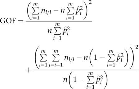is appealing, where n is the sample size, n_i/j is the number of observed genotypes of type i/j, and p̂_i is the gene counting estimate of the allele frequency p_i. Unfortunately, the GOF statistic does not follow a χ² distribution when the p_i are unequal.¹⁸ Weir¹⁸ suggests replacing the GOF test with the homozygosity test¹⁹

The test statistic H asymptotically follows a χ² distribution with one degree of freedom.¹⁹

Very few of the HWE tests have been extended to pedigree data. The obvious LRT extension compares the likelihood using arbitrary genotype frequencies for the founders to the likelihood using HW genotype frequencies for the founders. This test also has m(m−1)/2 degrees of freedom and suffers from overparameterization for large m. Bourgain et al.²⁰ developed a parsimonious quasi-score test that is parameterized by a heterozygous–homozygous fixation index.²¹ Their model does not readily lend itself to maximum likelihood estimation because of the complex bounds on the fixation index. Inspired by the Bourgain et al. model, we propose a model motivated by a simple acceptance–rejection mechanism. Our heterozygote–homozygote test (HH test) admits pedigree data, inbreeding internal to each pedigree and markers with dominant or recessive alleles (non-codominant markers). With no segregation distortion, complete typing of pedigree members, and a codominant marker, the HH test can dispense with the nonfounders in the pedigree and concentrate solely on the founders.

Heterozygote–homozygote model

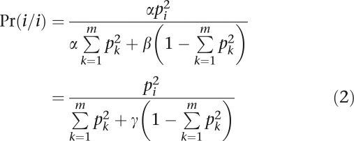
Suppose we are interested in testing HWE at a locus with m alleles and corresponding allele frequencies (p₁,…,p_m). In our model, we postulate that nature operates by first sampling the genotypes i/i and i/j with the usual HW probabilities and then subjecting a proposed genotype to an acceptance–rejection step. Let α be the acceptance probability for homozygotes, and let β be the acceptance probability for heterozygotes. If γ=β/α, then the various genotypes are ultimately accepted with the probabilities

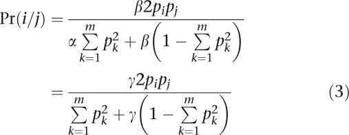The parameters α and β cannot both be estimated. This identifiability crisis is overcome by estimating their ratio γ. When the individuals in the sample are unrelated, then the distribution of the genotype count vector n=(n_1/1,…,n_1/m,…,n_m/m) is multinomial with likelihood proportional to

By declaring isolated individuals to be degenerate pedigrees, the model easily extends to samples consisting of independent pedigrees or mixtures of pedigrees and unrelateds. As the log-likelihoods of independent pedigrees add, it suffices to consider the likelihood of a single pedigree. If this pedigree has s members, then the likelihood formula

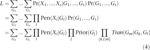of Ott²² applies, where X_i is person i's marker phenotype and G_i is his/her marker genotype. The product on j is taken over all founders, and the product on {k,l,m} is taken over all parent–offspring triples. The prior Prior(G_j) is given by Eq. (2) or (3). The penetrance for a marker Pen(X∣G) is either zero or one. The transmission probability Tran(G_m∣G_k,G_l) follows the traditional Mendelian law of independent segregation.

Computational efficiency is improved by lumping the alleles not seen in a pedigree. Our implementation of the HH test in the pedigree analysis package Mendel²³ employs a combination of genotype elimination²⁴ and allele lumping.²³ Alleles observed in a pedigree are preserved; the remaining alleles are lumped. Computation of founder priors must be performed carefully to preserve the correct form of the likelihood (Eq. (4)). Suppose the first k alleles are observed, and the remaining m-k alleles are missing in a pedigree. Eqs. (2) and (3) hold without modification for founder genotypes formed from the k observed alleles. Let q denote the lumped allele, and let

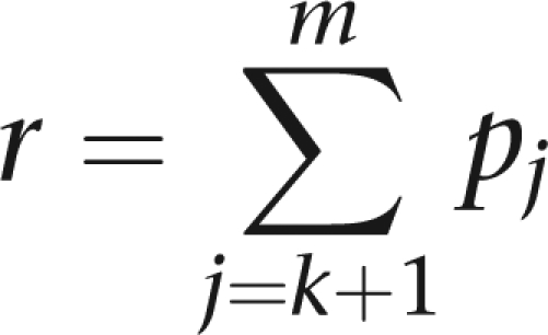denote its frequency. To account for lumping, we adjust the remaining genotype probabilities as follows:

The numerator of Eq. (5) accounts for the fact that genotype q/q is a composite of homozygous and heterozygous genotypes.

We maximize the sum of the log-likelihoods subject to the constraints 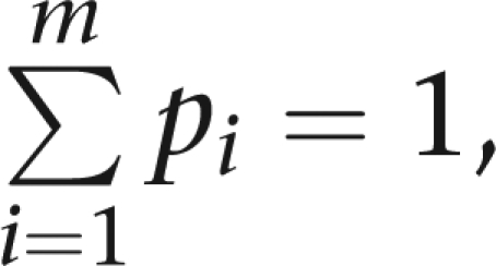p_i≥0, and γ≥0. In our computer program Mendel,²³ maximum likelihood estimation is accomplished efficiently by a quasi-Newton algorithm. To form the likelihood ratio statistic, we maximize the log-likelihood both under the null hypothesis (γ=1) and the alternative hypothesis (γ≠1). Under the null hypothesis, twice the difference in the two maximum log-likelihoods follows an asymptotic χ² distribution with one degree of freedom.

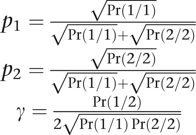
For a biallelic marker, the HH test is fully equivalent to the LRT based on genotypes. Proof of this fact just boils down to showing that one model is a reparameterization of the other. We have already demonstrated how to pass from the allele frequencies p₁ and p₂ and ratio γ of our model to the genotype probabilities Pr(1/1), Pr(1/2), and Pr(2/2) of the standard model. The reverse transformation simply amounts to

Type-one error rate and power

Now that we have presented our basic theory, we concentrate on demonstrating the flexibility of the HH test and on showing that it has the appropriate type-one error rates and comparable power to the Homozygosity test (H test). To address the question of type-one error rates, we simulated 1000 datasets under the null hypothesis of HWE. Each dataset includes 100 unrelated individuals typed at a marker with four equally frequent alleles. Using a significance level of 0.05, we find that the HH test has a type-one error rate of 0.047 (SD=0.007). In comparison, the benchmark H test has a type-one error rate of 0.042 (SD=0.006).

To assess the power of the HH test to detect deviations from HWE, we conducted two sets of simulations under our model. Each involved (a) a codominant marker with four alleles, (b) a grid of γ values ranging from 0.31 to 3.0, and (c) 1000 trials at each grid point. The first set of simulations used 100 unrelated individuals and assumed equally frequent alleles; the second used 200 unrelated individuals and assumed the allele frequency vector (0.8, 0.1, 0.05, 0.05). We chose these conditions so that in both cases the power was similar, approximately 0.80, when γ=2. As power depends on allele frequencies, we had to double the sample size for the skewed allele frequencies.

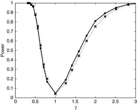
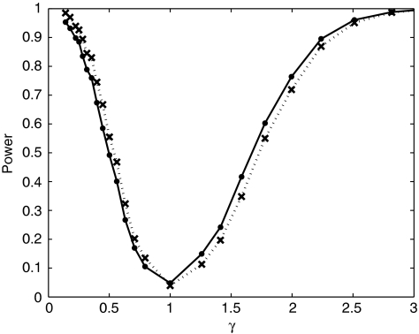
To generate genotypes under the alternative hypothesis γ≠1, we sampled with replacement as dictated by the model. This was realized for γ<1 by defining the acceptance probabilities α=1 and β=γ and for γ≥1 by defining α=1/γ and β=1. Genotypes were successively sampled for each individual until the first acceptance. We computed power at each grid point as the fraction of the datasets that reject the null hypothesis at the 0.05 level. Figure 1 plots power as a function of γ for both the HH test (solid line) and the H test (dashed line) for equally frequent alleles; Figure 2 does the same for the allele frequency vector (0.8, 0.1, 0.05, 0.05). For both sets of simulation conditions, the power curves of the H test and the HH test are not substantially different. At the point γ=1, both tests continue to show the correct type-one error rate.

Figure 1.

Comparison of the power of the HH and H tests with equally frequent alleles. Results of simulations to determine power as a function of γ. Each simulation is comprised of 1000 datasets each with n=100 unrelated individuals and 4 equally frequent alleles. The solid line denotes the power of the HH test. The dotted line denotes the power of the H test.

Figure 2.

Comparison of the power of the HH and H tests with skewed allele frequencies. Results of simulations to determine power as a function of γ. Each simulation is comprised of 1000 datasets with n=200 unrelated individuals and allele frequency vector=(0.8, 0.1, 0.05, 0.05). The solid line denotes the power of the HH test. The dotted line denotes the power of the H test.

A robust test should also possess good power against alternatives not covered by the model. We accordingly simulated another 1000 datasets with (a) n=200 unrelated individuals, (b) 3 codominant alleles with frequencies p₁=0.5 and p₂=p₃=0.25, and (c) acceptance probabilities α_1/1=1.0, α_2/2=0.5, α_3/3=0.25, β_1/2=1.0, β_1/3=0.5, and β_2/3=0.25. In these datasets, the rejection rate for the H test is 0.328 and the rejection rate for the HH test is 0.343.

In practice, violations of HWE often stem from population stratification. We therefore conducted 100 simulations combining 100 random individuals from each of two different populations separately in HWE. In population 1 the frequency vector of the three codominant alleles is (0.4, 0.3, 0.3); in population 2 it is (0.8, 0.1, 0.1). If we keep the two sets of 100 individuals separate, the average estimated γ in the first set is 0.99 and 1.07 in the second set. When we analyze the combined datasets, the averaged estimated γ is 0.71. In 86 out of the 100 combined datasets, the HH test has a P value less than 0.05.

Finally to validate the HH test in family data, we simulated nuclear families with missing founder genotypes. Specifically we simulated 1000 sets of 100 nuclear families under various scenarios. Each simulation scenario assumed (a) 3 fully genotyped siblings, (b) a codominant marker with 3 alleles, and (c) the allele frequency vector (0.5, 0.25, 0.25). In the first scenario, we took γ=1. In this case the type-one error rate is 0.046 and the average estimate of γ is 1.07, with 95.2% of the 95% confidence intervals covering γ=1 (95% coverage rate =95.2%.) In the second scenario γ=1.5. Here the average estimate of γ is 1.64 and the 95% coverage rate is 93.0%. In the third scenario γ=0.50. Now the average estimate of γ is 0.52 and the 95% coverage rate is 93.4%. These results appear reasonable.

Real data examples

It is also revealing to consider real data. Our first example involves the classical survey by Waaler^{25, 26} of X-linked recessive color blindness. These European data consist of 40 affected women, 725 affected men, 9032 unaffected women, and 8324 unaffected men. We analyze the data assuming that the color-blindness locus has two alleles, d and D, and that men with genotype d and women with genotype d/d are color blind. The likelihood contributions for affected and unaffected men are p_d and p_D, respectively. Note that these contributions do not depend on γ. The likelihood of an affected woman is

An unaffected woman is either a D/D homozygote or a D/d heterozygote. Thus the likelihood of an unaffected woman is

As all individuals are unrelated, the likelihood for the full data is

Our computer program Mendel can maximize likelihoods of this sort involving dominant and recessive alleles. All the user needs to do is define the X-linked locus as non-codominant in Mendel's definition file. Details can be found in the Mendel manual available at the UCLA web site mentioned later.

One of the virtues of the HH test on this problem is that it correctly incorporates allele frequency information contributed by men. The estimate γ̂=4.087 (SD=1.661), and corresponding likelihood ratio statistic of 5.119 output by Mendel give an asymptotic P value of 0.0237. This apparent violation of HWE is hardly surprising because there are actually two different forms of color blindness, protanopia and deuteranopia, located on the X chromosome.

As a more computationally challenging example, we now consider 1296 highly polymorphic markers on chromosomes 1, 2, and 3 deposited in the CEPH database version 10 (website: www.cephb.fr/cephdb/). The number of families, individuals, founders, and missing founder genotypes vary from marker to marker. The minimum number of genotyped families is 8, the minimum number of genotyped individuals is 84, and the minimum number of genotyped founders is 24. The maximum number of families is 40, the maximum number of genotyped individuals is 510, and the maximum number of genotyped founders is 131. To avoid needless computation, we trimmed ungenotyped family members unless they were critical in determining relationships between genotyped family members.²⁷ We also removed all Mendelian genotyping errors.^{8, 23, 24, 28} Under suboption 1 of the Mistyping option of Mendel, evidence of a genotyping error at a particular marker in a particular family causes the program to delete all genotypes at the marker in the family.

Testing of HWE is conducted by comparing maximum likelihoods under the null hypothesis (H_o: γ=1) and the alternative hypothesis (H_a: γ unrestricted). In both cases allele frequencies are estimated. The usual likelihood ratio statistic

asymptotically follows a χ² distribution with one degree of freedom. For problems involving this many markers, Mendel takes tens of minutes of computing time. Exact times depend on the computing platform and compiler.

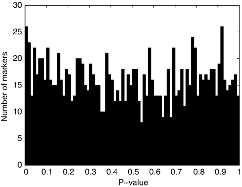
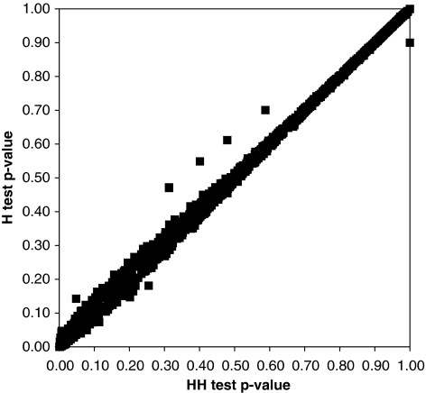
The resulting histogram of P values is shown in Figure 3. Except for a small spike near 0, the distribution appears uniform. Figure 4 compares H and HH P values based on founders alone. As expected from our previous simulation results, P values under the two tests are similar. As the HH test estimates allele frequencies as well as the heterozygote/homozygote ratio γ, it can provide a more sensitive test of HWE when an excess in the number of homozygous genotypes of one kind is balanced by a deficit in the number of homozygous genotypes of another kind. Violation of HWE in this situation is masked in the H test because the test statistic uses only the total counts of heterozygotes and homozygotes.¹⁸

Figure 3.

The distribution of HH test P values using data from the CEPH families. The results are from 1296 markers, each with 3 to 26 alleles. The number of families ranges from 8 to 40, the number of genotyped founders ranges from 24 to 131, and the number of genotyped individuals ranges from 84 to 510.

Figure 4.

Comparison of the HH test and H test P values using the genotyped founders from the CEPH families. The results are for the same 1296 highly polymorphic markers genotyped in the CEPH families (Figure 3). The number of unrelated individuals ranges from 24 to 131.

Finally, we illustrate the versatility of the HH test in handling tightly linked SNPs. Combining neighboring SNPs is a standard tactic for increasing their information content. When HWE holds, the frequency of the multi-locus phenotypes remain constant from generation to generation and can be predicted using haplotype frequencies. Owing to phase uncertainties, the supermarkers constructed from tightly linked SNPs are non-codominant.

For the sake of simplicity, let us consider the case of two neighboring SNPs. More SNPs can be handled by the same tactics. We denote a bi-locus phenotype as i₁i₂j₁j₂, where i₁/i₂ is the unordered genotype at the first SNP and j₁/j₂ is the unordered genotype at the second SNP. There are nine possible phenotypes. The corresponding alleles are the four haplotypes, 1-1, 1-2, 2-1, and 2-2. Eight of the nine bi-locus phenotypes correspond to a single haplotype pair. For example, the bi-locus phenotype 1112 is consistent with only the single haplotype pair 1-1/1-2. The doubly heterozygous phenotype 1212 is consistent with the two haplotype pairs 1-1/2-2 and 1-2/2-1. To convert two tightly linked SNPs into one non-codominant marker with four alleles, one can use the Combining_Loci option of Mendel.^{23, 29} The Mendel manual supplies the full syntax for constructing input files and interpreting output files.

As discussed in the X-linked color-blindness example, non-codominant markers can be easily handled in computing the pedigree likelihood (Eq. (4)); one simply sums over all possible genotypes consistent with each observed marker phenotype.

For example with a supermarker constructed from two neighboring SNPs, whenever an individual with phenotype 1212 is encountered, both of the genotypes 1-1/2-2 and 1-2/2-1 are visited in likelihood calculation. The priors shown in Eqs. (2) and (3), the null hypothesis (γ=1), and the alternative hypothesis (γ unrestricted) are interpreted exactly the same regardless of whether a marker is codominant or not. As an example, we combined SNPs rs998132 and rs434410 in the CEPH data. Although these two SNPs are approximately 3.5 Mb apart, no recombination events are observed between them. Table 1 summarizes our HH test results with the combined markers. Notice here that the evidence against HWE increases when we analyze the two markers together.

Table 1. Combined SNP results.

Marker name	γ̂	SE	HH P-value
rs998132	0.5132	0.1590	0.0274
rs434410	0.4322	0.1603	0.0206
Combined	0.3401	0.1085	0.0011

Discussion

In summary, the HH test has the advantages of allowing (a) a mixture of pedigree and random sample data, (b) non-codominant markers, and (c) highly polymorphic markers. It is motivated by a simple to understand acceptance–rejection model. It is slightly conservative and almost always as powerful as the benchmark H test. In some settings, for example in pedigree data with untyped founders, it is more powerful than the H test. The HH test does entail considerably more computing, but this is hardly a consideration for moderate-sized datasets. Inbred children are allowed but not inbred or related founders. Mendelian segregation is assumed to hold in the transmission of genes from parent to offspring. If departures from these assumptions are suspected of occuring, the methods of Bourgain et al.²⁰ will be more appropriate.

The HH test is now implemented in the publicly available software package Mendel (version 9.0 or later at www.genetics.ucla.edu/software) as part its Allele_Frequencies option. The option is fully documented and illustrated by specific numerical examples. We hope that this free software implementation will prove attractive to users.

References

- Hardy GH. Mendelian proportions in a mixed population. Science. 1908;28:49–50. doi: 10.1126/science.28.706.49. [DOI] [PubMed] [Google Scholar]
- Weinberg W. Über den nachweis der verrebung bein menschem. Jahresh Verein. 1908;64:368–382. [Google Scholar]
- Stern C. The Hardy-Weinberg law. Science. 1943;97:137–138. doi: 10.1126/science.97.2510.137. [DOI] [PubMed] [Google Scholar]
- Casellas J. Survival QTL fine-mapping by measuring and testing for Hardy-Weinberg and linkage disequilibrium. Genetics. 2007;176:721–724. doi: 10.1534/genetics.106.067264. [DOI] [PMC free article] [PubMed] [Google Scholar]
- Nielsen D, Ehm MG, Weir BS. Detecting marker-disease association by testing for Hardy-Weinberg disequilibrium at a marker locus. Am J Hum Genet. 1999;63:1531–1540. doi: 10.1086/302114. [DOI] [PMC free article] [PubMed] [Google Scholar]
- Lee WC. Searching for disease-susceptibility loci by testing for Hardy-Weinberg disequilibrium in a gene bank of affected individuals. Am J Epidemiol. 2003;158:379–400. doi: 10.1093/aje/kwg150. [DOI] [PubMed] [Google Scholar]
- Wittke-Thompson JK, Pluzhnikov A, Cox NJ. Rational inferences about departures from Hardy-Weinberg equilibrium. Am J Hum Genet. 2005;76:967–986. doi: 10.1086/430507. [DOI] [PMC free article] [PubMed] [Google Scholar]
- Douglas JA, Skol AD, Boehnke M. Probability of detection of genotyping errors and mutations as inheritance inconsistencies in nuclear-family data. Am J Hum Genet. 2002;70:487–495. doi: 10.1086/338919. [DOI] [PMC free article] [PubMed] [Google Scholar]
- Sen S, Burmeister M. Hardy-Weinberg analysis of a large set of published association studies reveals genotyping error and a deficit of heterozygotes across multiple loci. Hum Genomics. 2008;3:36–52. doi: 10.1186/1479-7364-3-1-36. [DOI] [PMC free article] [PubMed] [Google Scholar]
- Elston RC, Forthofer R. Testing for Hardy-Weinberg equilibrium in small samples. Biometrics. 1977;33:536–542. [Google Scholar]
- Emigh TH. A comparison of tests for Hardy-Weinberg equilibrium. Biometrics. 1980;36:627–642. [PubMed] [Google Scholar]
- Hernandez JL, Weir BS. A disequilibrium coefficient approach to Hardy-Weinberg testing. Biometrics. 1989;45:43–70. [PubMed] [Google Scholar]
- Guo SW, Thompson EA. Performing the exact test of Hardy-Weinberg proportions for multiple alleles. Biometrics. 1992;48:361–372. [PubMed] [Google Scholar]
- Weir BS. Genetic Data Analysis 2: Methods for Discrete Population Genetic Data. Sunderland, MA: Sinauer Associates Inc.; 1996. [Google Scholar]
- Chen JJ, Thomson G. The variance of the disequilibrium coefficient in the individual Hardy-Weinberg test. Biometrics. 1999;55:1269–1272. doi: 10.1111/j.0006-341x.1999.01269.x. [DOI] [PubMed] [Google Scholar]
- Chen JJ, Duan T, Single R, Mather K, Thomson G. Hardy-Weinberg testing of a single homozygous genotype. Genetics. 2005;170:1439–1442. doi: 10.1534/genetics.105.043190. [DOI] [PMC free article] [PubMed] [Google Scholar]
- Lee CC, Horvitz DG. Some methods of estimating the inbreeding coefficient. Am J Hum Genet. 1953;5:107–117. [PMC free article] [PubMed] [Google Scholar]
- Weir BS. Independence of VNTR Alleles defined as fixed bins. Genetics. 1992;130:873–887. doi: 10.1093/genetics/130.4.873. [DOI] [PMC free article] [PubMed] [Google Scholar]
- Barker JS, East PD, Weir BS. Temporal and micrographical variation in allozyme frequencies in a natural population of Drosophila buzzatii. Genetics. 1986;112:577–611. doi: 10.1093/genetics/112.3.577. [DOI] [PMC free article] [PubMed] [Google Scholar]
- Bourgain C, Abney M, Schneider D, Ober C, McPeek MS. Testing for Hardy-Weinberg equilibrium in samples with related individuals. Genetics. 2004;168:2349–2361. doi: 10.1534/genetics.104.031617. [DOI] [PMC free article] [PubMed] [Google Scholar]
- Rousset F, Raymond M. Testing heterozygotes excess and deficiency. Genetics. 1995;140:1413–1419. doi: 10.1093/genetics/140.4.1413. [DOI] [PMC free article] [PubMed] [Google Scholar]
- Ott J. Estimation of the recombination fraction in human pedigrees: efficient computation of the likelihood for human linkage studies. Am J Hum Genet. 1974;26:588–597. [PMC free article] [PubMed] [Google Scholar]
- Lange K, Cantor R, Horvath S, et al. Mendel version 4.0: a complete package for the exact genetic analysis of discrete traits in pedigree and population data sets. Am J Hum Genet. 2001;69S1:504. [Google Scholar]
- Lange K, Goradia TM. An algorithm for automatic genotype elimination. Am J Hum Genet. 1987;40:250–256. [PMC free article] [PubMed] [Google Scholar]
- Crow JF.Basic Concepts in Population, Quantiative, and Ecological Genetics. San Francisco: Freeman; 1986 [Google Scholar]
- Waaler GHM. Uber die Erblichkeitsverhaltnisse der verschiedenenArten von angeborener Rotgrunblindheitrdquo. Z Indukt Abstamm Vererbungsl. 1927;45:279–333. [Google Scholar]
- Lange K, Sinsheimer JS. The pedigree trimming problem. Hum Hered. 2004;58:108–111. doi: 10.1159/000083031. [DOI] [PubMed] [Google Scholar]
- Sobel E, Papp JC, Lange K. Detection and integration of genotyping errors in statistical genetics. Am J Hum Genet. 2002;70:496–508. doi: 10.1086/338920. [DOI] [PMC free article] [PubMed] [Google Scholar]
- Sinsheimer JS, McKenzie CA, Keavney B, et al. SNPs and snails and puppy dogs' tails: analysis of SNP haplotype data using the gamete competition model. Ann Hum Genet. 2001;65:483–490. doi: 10.1017/S0003480001008843. [DOI] [PubMed] [Google Scholar]