Frequency response of lift control in Drosophila

Abstract

The flight control responses of the fruitfly represent a powerful model system to explore neuromotor control mechanisms, whose system level control properties can be suitably characterized with a frequency response analysis. We characterized the lift response dynamics of tethered flying Drosophila in presence of vertically oscillating visual patterns, whose oscillation frequency we varied between 0.1 and 13 Hz. We justified these measurements by showing that the amplitude gain and phase response is invariant to the pattern oscillation amplitude and spatial frequency within a broad dynamic range. We also showed that lift responses are largely linear and time invariant (LTI), a necessary condition for a meaningful analysis of frequency responses and a remarkable characteristic given its nonlinear constituents. The flies responded to increasing oscillation frequencies with a roughly linear decrease in response gain, which dropped to background noise levels at about 6 Hz. The phase lag decreased linearly, consistent with a constant reaction delay of 75 ms. Next, we estimated the free-flight response of the fly to generate a Bode diagram of the lift response. The limitation of lift control to frequencies below 6 Hz is explained with inertial body damping, which becomes dominant at higher frequencies. Our work provides the detailed background and techniques that allow optomotor lift responses of Drosophila to be measured with comparatively simple, affordable and commercially available techniques. The identification of an LTI, pattern velocity dependent, lift control strategy is relevant to the underlying motion computation mechanisms and serves a broader understanding of insects' flight control strategies. The relevance and potential pitfalls of applying system identification techniques in tethered preparations is discussed.

1. Introduction

Flying insects perform impressive flight manoeuvres that remain unmatched by micro-robotic systems (for a review, see Floreano et al. 2009; table 1). The remarkable flight control abilities are achieved from a close integration of multimodal sensory processing and sophisticated motor control (reviewed e.g. by Dickinson 2006), which promise new biomimetic design principles suitable for the control of autonomous navigating micro-air vehicles (MAVs: e.g. Schenato et al. 2004; Zufferey & Floreano 2006; Franceschini et al. 2007; Floreano et al. 2009).

Table 1.

Nomenclature

A, Ain	pattern oscillation amplitude (peak-to-peak) (m)
Aest	oscillation amplitude of estimated free-flight position (m)
Aforce	oscillation amplitude of measured lift force (N)
ɛ	pixel spacing of LED display (m)
f	pattern oscillation frequency (Hz)
frefresh	refresh rate of LED display (s−1)
Flift	lift force produced by the fly (N)
FMEMS	force applied by the fly on the sensor probe (N)
G	gain between pattern position and fly position
g	gravitation constant (m s−2)
I, Imax, Imin	dimensionless light intensity of LED display (1)
Λ	pattern linear wavelength (m)
m	mass of the fly (kg)
p	pattern position (m)
pest	estimated vertical position of the fly (m)
Δφ	phase difference between pattern position and fly position (deg)
SF	pattern linear spatial frequency (m−1)
sf	pattern angular spatial frequency (deg−1)
sfmin	minimal SF as viewed at the horizon (deg−1)
TF	pattern temporal frequency (s−1)
V	pattern linear velocity (m s−1)

To stabilize flight, flies, like other flying insects, are required to quickly react to perceived perturbations with appropriate corrective steering manoeuvres, which are mediated by reflexive sensorimotor pathways (recent reviews: Krapp 2000; Frye & Dickinson 2004; Dickinson 2006; Egelhaaf 2008).

Functional insights into neuromotor control pathways can be gained by studying their input–output relationships at a behavioural level, applying a so-called black-box approach (Poggio & Reichardt 1973). System identification techniques (applied to flight control in the fruitfly, e.g. Epstein et al. 2007, Dickson et al. 2008; Fry 2009; Rohrseitz & Fry submitted) provide a solid analytical framework based on rigorous engineering principles. Such a system analysis does not require a detailed understanding of the highly complex and only partially understood neuromotor control mechanisms underlying the studied reflex.

A behavioural systems analysis approach requires precise control over the sensory inputs to the biological system and a measurement of the motor output relevant to the behavioural context. Tethered preparations of walking or flying insects provide an elegant solution to this problem, in that sensory stimuli can be delivered in a defined manner, while measuring the intended corrective steering responses from the movements of the wings or legs (open-loop condition: Hassenstein & Reichardt 1956; review: Buchner 1984). In tethered flying Drosophila, for example, open-loop preparations have been extensively applied to characterize optomotor responses to large-field pattern motion (e.g. Götz 1968; Tammero & Dickinson 2002), which under natural free-flight conditions is induced by the fly's movements within the environment (optic flow: Gibson 1958). The behaviourally measured open-loop response characteristics can provide insight into the underlying neuromotor control mechanisms and flight dynamics (Taylor & Krapp 2008).

Most measurements of visual flight control responses have so far been performed under steady-state conditions, providing detailed insights e.g. into the visual transduction process. Steady-state conditions do not reflect the highly dynamic stimulus conditions experienced by freely flying flies (Schilstra & van Hateren 1998, 1999; review: Egelhaaf & Kern 2002) and are in principle unsuited to characterize the dynamics of a control system. In contrast, behavioural responses in the presence of time-varying stimuli can be measured to characterize transient response dynamics at the time scales relevant for flight control. Such dynamic stimuli can consist, e.g., of step-inputs of pattern motion (Borst & Bahde 1986; Fry et al. 2009) or oscillating patterns (Sherman & Dickinson 2003; Duistermars et al. 2007).

A frequency response analysis takes this approach further, in that the animal's response to a temporally periodic stimulus is measured over a broad range of oscillation frequencies. The gain and phase delay of the responses can then be represented as a Bode plot (Nise 2004), which provides information about the controller's bandwidth and cutoff frequency. Recently, Tanaka & Kawachi (2006) characterized lift responses of tethered flying bumblebees (Bombus terrestris) elicited with vertically oscillating patterns and compared the bee's performance with that of human-controlled aircraft. Bode plots have also been previously used to characterize frequency responses in free-flying insects in the context of lift control (Drosophila hydei: David 1984) and station keeping (Macroglossum stellatarum: Farina et al. 1994). In these cases, the experiments were performed under closed-loop conditions and the visual inputs were calculated from the stimulus conditions and the insects' measured responses.

The abstraction of optomotor response dynamics in Bode diagrams is intriguing, as it provides a common conceptual framework to compare response dynamics across different measurement conditions, among different animal species and between biological and technological systems.

Despite its appeal, the application of abstract system identification approaches in biological systems is non-trivial and prone to misconceptions. First, many system identification techniques depend on the linearity and time-invariance (LTI) of the control system considered. In the case of biological control systems, there is no basis to presume LTI characteristics a priori. In the case of visual flight control of flies, for example, existing models of motion processing predict strongly nonlinear response characteristics (review, e.g., Borst & Haag 2002). On the other hand, there is growing evidence that insects achieve robust flight control from a piecewise nonlinear flight control system that has evolved to be linear at the top level (Taylor & Krapp 2008). The important question whether optomotor responses of insects reveal LTI characteristics (Theobald et al. 2010) remains to be examined explicitly. Second, experimental constraints required to make precise measurements may render them difficult to interpret. In the case of tethered flight experiments, for example, attaching an insect to a tether precludes a direct measurement of the body kinematics and is the cause for substantial behavioural artefacts (Fry et al. 2005). A detailed analysis of the response properties is therefore required to verify the feasibility of a frequency response analysis. Third, the control inputs and outputs of the biological controller—unlike in engineered systems—are a priori unknown and first needs to be identified. A controller based on linear velocity was recently identified for forward flight speed control in Drosophila (Fry et al. 2009; Rohrseitz & Fry submitted), the control variable in the case of lift control has so far not been tested explicitly. A system analysis approach therefore not only offers tools and concepts to analyse biological controllers, it also raises fundamental questions about the underlying control system that might otherwise not be considered.

The fruitfly Drosophila represents a powerful model system to explore neuromotor control mechanisms due to the detailed knowledge of its neuromotor pathways and the ability to easily measure behavioural responses under tethered flight conditions. Motivated by our interest in the control of translatory flight and its underlying visuomotor processes, we extended the approach of Tanaka & Kawachi (2006) with a broader and more detailed analysis of lift control in the fruitfly. In particular, we wanted to test the hypothesis that lift responses, like flight speed responses (Fry et al. 2009; Rohrseitz & Fry submitted), are largely invariant to the pattern spatial frequency (SF), a question of high relevance in view of the neural motion processing pathways presumed to underlie optomotor responses in flies (reviewed, e.g., by Borst & Haag 2002). For the sake of a direct comparison with previous analyses in biological and engineering systems, we closely followed the approach of Tanaka & Kawachi (2006). Given the broader relevance of behavioural system identification techniques, we explain in detail the approach taken and address various critical issues related to it.

We performed the force measurements using well-characterized micro-electro-mechanical systems (MEMS) force sensors (Graetzel et al. 2008a,b). By systematically varying the pattern oscillation amplitude (A) and spatial frequency (SF), we explored the dynamic range of lift responses. We also explicitly tested the LTI assumption of the lift response within the dynamic range, including the superposition and homogeneity properties of the system. We then characterized the lift response properties with an analysis of amplitude gain and phase responses. Finally, we developed an inertial model to estimate the fly's ‘free-flight’ body position, tested its validity for the frequency range tested and used it to characterize the lift response dynamics in form of a Bode plot.

We found that lift control in Drosophila is velocity dependent and meets the requirements of an LTI system well within the dynamic range. The response dynamics are well explained with a constant response delay of about 75 ms and the inertial body dynamics, which tend to dampen out higher frequencies. The Bode plot shows strong disturbance rejection at low frequencies followed by a drop-off caused by body inertia. Besides providing insight into visuomotor lift control, our work provides a conceptual framework to perform a meaningful frequency response analysis. The limitations and broader relevance of the approach are discussed.

2. Material and methods

Fruitflies (Drosophila melanogaster, Meigen) were obtained from a stock descended from a wild-caught population of 200 mated females. A standard breeding procedure was adopted, in which flies were bred from 25 females and 10 males and reared on standard nutritive medium on a 12 h : 12 h light/dark cycle. For the measurements we used 2–4 day old female flies. Experiments were performed during the first 6 h of subjective day.

To measure a fly's lift forces, we tethered it to a custom built, commercially available MEMS force sensor (FT-S540, Femtotools GmbH, Zurich, Switzerland; www.femtotools.com). The sensor reading provides the total lift force produced by the fly minus its weight. Positive and negative forces therefore correspond to a net vertical force that would cause the fly to accelerate upwards or downwards, respectively. The MEMS sensors were carefully calibrated with a reference sensor and verified with micro-scale readings. The validity of force readings with these sensors were confirmed in many other experiments carried out by Femtotools, and applied in previous studies to measure tethered flight forces in Drosophila (Sun et al. 2005; Graetzel et al. 2008a,b).

The sensor was connected to custom built electronic read-out electronics, whose force-dependent analogue output voltage we sampled at 10 kHz and a 16 bit/10 V resolution using a CompactRIO device (National Instruments Corp., Austin, TX, USA; www.ni.com). The chosen sensor had a range of 160 μN, a resolution of 0.05 μN and a resonant frequency of 1000 Hz. To remove potential artefacts caused by the sensor's resonance, we dynamically calibrated the force sensor in a laser vibrometer (Polytec GmbH, www.polytec.com). The frequency response of the sensor was inverted and applied to the raw data to filter out dynamic effects.

The tethering procedure consisted of immobilizing the fly in a refrigerator (4°C) and transferring it onto a custom built, thermoelectrically cooled (4°C) manipulation stage. The fly was placed on a movable semi-sphere that allowed a precise adjustment of the body orientation. We then deposited a droplet (diameter approx. 50 μm) of UV-curing glue (Loctite, Duro Clear Glass Adhesive) on the fly's thorax, brought the MEMS sensor probe in contact with the glue using a Sutter MP-285 micro-positioning stage (Sutter Instrument, Novato, CA, USA; www.sutter.com) and cured the glue with a UV lamp (ELC305, Electro-Lite Corp., Bethel, CT, USA; www.electro-lite.com). The tethering angle was adjusted such that when the sensor was vertical, the body angle formed a 45° angle with respect to the horizon. The fly was given at least 10 min to recover before conducting measurements.

Fruitflies maintain a constant mean force vector with respect to their body (Götz 1968). Consequently, their forward flight speed is closely coupled to their body orientation (David 1978), while a constant body posture is maintained during hovering (about 45° in D. melanogaster, Fry et al. 2003). Vertical control in hovering flies is mediated by changes in stroke frequency and amplitude (Lehmann & Dickinson 1997), but is not accompanied by detectable changes in body attitude (also see supplementary video in Fry et al. 2003).

The MEMS sensor with the fly attached to it was then placed at the centre of a 75 mm radius cylindrical display (figure 1) constructed from 60 modules, each consisting of an 8 × 8 array of green light emitting diodes (LED). For details on the modular display system refer to Reiser & Dickinson (2008). We controlled the eight luminance values of each LED with a refresh rate of 60 Hz using a CompactRIO real-time FPGA controller, which we programmed using LabVIEW (National Instruments Corp.; www.ni.com). The publication time of the patterns was logged as a reference for the subsequent analysis of the force data. The angular displacement between adjacent LEDs was 3.65°. For additional details on the LED arena see Graetzel et al. (2008b).

Figure 1.

Measurement set-up. A cylindrical arena was constructed from 60 modular LED panels. Lift forces were measured from flies flying tethered to a MEMS (micro-electro-mechanical systems) force sensor (see inset), which we placed in the middle of the arena. The flies were stimulated using vertically oscillating horizontal sine grating patterns, whose spatial frequency we varied systematically between trials. Oscillation amplitude and frequency were also varied systematically.

For the main experiments, we used vertically oscillating horizontal sine gratings, whose linear SF (in m⁻¹) we varied systematically (for definitions of linear and angular pattern parameters see Fry et al. 2008, 2009; for a list of symbols used in this article see table 1). The position of the pattern in time is described as:

2.1

where A is the peak-to-peak oscillation amplitude and f is the frequency of oscillation. The stimulus conditions therefore depended on three parameters: SF, A and f, each of which we varied systematically in our experiments. An overview of the parameters in linear and angular units is provided in table 2.

Table 2.

Measurement parameters. f and A are pattern oscillation frequency and amplitude, respectively. SF is the linear spatial frequency, sf_min is the minimal angular spatial frequency as viewed by the fly at the horizon (zero elevation). Above and below the horizon, the angular spatial frequency SF is increased due to geometric distortion.

f	0.1–13 (Hz)
A	2.38; 4.76; 7.14 (10−2 m)
SF	1.05; 1.58; 2.10; 2.62 (101 m−1)
sfmin	1.54; 2.18; 2.84; 3.51 (10−2 deg−1)

To test the fly's response to the superposition of two frequency inputs, we also oscillated sine grating patterns with two different oscillation frequencies superimposed:

2.2

The 60 Hz refresh rate of the display limited the oscillation frequencies and amplitudes that we could display without artefacts. Spatio-temporal aliasing occurs if a pattern shifts more than half its wavelength between frames. To avoid aliasing, the pattern temporal frequency TF (the instantaneous ‘flicker’ frequency of any pixel, in s⁻¹) must lie below half the refresh rate (Nyquist frequency):

2.3

The limits for un-aliased pattern presentation can be calculated by considering the fastest instantaneous motion of the oscillating pattern,

2.4

which depends on the product of oscillation amplitude and oscillation frequency. The linear velocity V (in m s⁻¹) of a sine grating pattern corresponds to the ratio of its TF and SF:

2.5

Combining equations (2.3)–(2.5), we see that a pattern will not shift more than half its wavelength if

2.6

This limit is conservative, because velocities near V_max are reached only during short periods of the cycle. All our measurements were performed well below the limits of spatio-temporal aliasing.

The display also provided limits to the spatial frequencies that we could display without artefacts. Spatial aliasing occurs if the pattern wavelength Λ falls below twice the spatial resolution of the screen

2.7

where ɛ is the pixel spacing of 4.76 × 10⁻³ m. Given these dimensions, the upper limit of SF is calculated at 105.0 m⁻¹. The highest SF used in our measurements was 26.2 m⁻¹.

The intensity I of each row of pixels y is based on the properties of the sinusoidal grating and of the oscillation. The intensity is discretized along the eight available relative luminance levels:

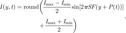2.8

where I_max is the highest relative intensity (in our case 7), I_min the smallest relative intensity (in our case 0). These relative luminance values correspond to increasing absolute luminance, as described in Reiser & Dickinson (2008). At high spatial frequencies, the discretization gets coarser because there are not enough pixels within a wavelength to use all greyscale values. We minimized the effect of the spatial discretization by using a real-time analytical calculation of the sinusoidal grating that determined the optimal quantization for each pixel. This anti-aliasing procedure leads to a smoother movement of the pattern compared to shifting a pre-calculated bitmap of the sine grating up or down by one pixel.

3. Results

3.1. Correspondence between stimulus and response

A close correspondence between the sinusoidal pattern oscillation and the lift forces produced by the fly is a prerequisite for a meaningful frequency response analysis. Examples of lift responses of four flies to an oscillating pattern (SF = 21.0 m⁻¹; A = 4.76 × 10⁻² m; f = 1 Hz) are shown in figure 2a. The lift forces follow the sinusoidal pattern motion quite closely, though higher frequency components are also present in the signal. In one example (red trace), the fly's forces deviate quite substantially from a perfectly sinusoidal response. The shape of the response function and the potential for inter-individual differences must therefore be closely considered to perform a meaningful frequency response analysis.

Figure 2.

Examples of force data measurements. (a) Tracking of pattern oscillation. a(i) shows the position (solid line) and velocity (dashed line) of a vertically oscillating horizontal sine grating (peak-to-peak oscillation amplitude A = 4.76 × 10⁻² m; oscillation frequency f = 1 Hz; spatial pattern frequency SF = 21.0 m⁻¹, not shown). a(ii) shows the resulting lift forces measured from four flies. As in the following plots, force data were low-pass filtered with a zero-phase, 5th order Butterworth filter with a cutoff frequency of 40 Hz. (b) Dependence on oscillation amplitude. A fly was stimulated using oscillation amplitudes of 2.38, 4.76 and 7.14 × 10⁻³ m (b(i)). The measured lift forces are shown in red, green and blue, respectively (b(ii)). (c,d) Dependence on oscillation frequency. Pattern position (red trace) is plotted together with the measured lift force (in black) for oscillation frequencies (c) 1.6 and (d) 3.1 Hz. SF = 15.8 m⁻¹, A = 2.38 × 10⁻² m in either case.

The fly's response follows the pattern velocity with a short delay, consistent with the notion that pattern velocity is the relevant control input for lift responses (for flight speed responses see Fry et al. 2009; Rohrseitz & Fry submitted) rather than pattern position. For a system analysis it is irrelevant whether position or velocity is used as input/output units, and we chose a position-based analysis to be consistent with previous work (McRuer & Graham 1964; Tanaka & Kawachi 2006).

3.2. Oscillation amplitude

A meaningful frequency response analysis required a suitable choice of A, such that we were able to measure a strong response signal without substantial response saturation. The effect of varying A is exemplified in figure 2b, which shows the lift response (normalized to average) of a fly stimulated with a threefold range of A. Using the smallest oscillation amplitude (A = 2.38 × 10⁻² m), the fly showed a closely sinusoidal response with a force response amplitude A_force varying between ±1 μN (red trace). With a twofold increase in oscillation amplitude (A = 4.76 × 10⁻² m), the response amplitude increased accordingly, but the time course became slightly distorted (green trace). Finally, with a threefold increase in oscillation amplitude (A = 7.14 × 10⁻² m), the response became considerably distorted, apparently saturating at A_force ≈ ±2 μN. The dynamic range of the responses in our measurement was only approximately 20 per cent of that previously measured with a slowly varying motion stimulus (approx. 10 μN peak-to-peak amplitude; figure 2 in Lehmann & Dickinson 1997). It is possible, therefore, that much lower saturation levels limit the performance of flies at the typically much shorter time scales relevant to flight control, including e.g. take-off manoeuvres (Card & Dickinson 2008). Taking care to remain below saturation, we can nevertheless expect the response amplitude to increase monotonically with the amplitude of the oscillation.

3.3. Oscillation frequency

The final two examples show how lift responses depend on f. A roughly twofold increase in f caused a slight decrease in response amplitude and a slight increase in phase lag (figure 2c,d). Taken together, the examples in figure 2 show that for a suitable choice of the stimulus parameters the time course of the lift force closely follows the pattern amplitude. A detailed quantitative analysis of lift response characteristics is provided below.

3.4. Stimulation with varying oscillation amplitudes

The amplitude gain measured for varying f is a relevant parameter describing a system's dynamics. A meaningful calculation of a gain implies a linear correspondence between inputs and outputs, in this case A and A_force. We tested this explicitly by measuring the A_force for two different oscillation amplitudes, A₁ = 4.76 × 10⁻² m and A₂ = 2.38 × 10⁻² m. In case of the higher oscillation amplitude A₁, A_force decreased from 0.9 ± 0.5 × 10⁻⁶ N at f = 1 Hz to 0.2 ± 0.05 × 10⁻⁶ N at f = 6 Hz, above which it remained roughly constant (figure 3, black trace). In case of the lower oscillation amplitude A₂, A_force decreased from 0.7 ± 0.2 × 10⁻⁶ N to 0.2 ± 0.05 × 10⁻⁶ N in the same range of f. Taken together, the flies responded more strongly to the higher oscillation amplitude for f ≤ 5 Hz, above which the two responses were indistinguishable. For frequencies above 5 Hz, the response lost any correlation with the stimulus signal, probably reflecting the limit of the fly's controller. We can rule out that limits in the visual stimulation or in the force sensor are causing the noise pattern, as they operate at significantly higher frequencies and sensitivities (see §2). The decrease was roughly linear for both oscillation amplitudes, except for high oscillation amplitude and low frequencies, at which a slight saturation is apparent (figure 3b, black trace, f ≤ 2 Hz).

Figure 3.

Frequency response. Shaded areas show ± s.d. The oscillation frequency f was varied between 0.1 and 13 Hz (a–e) or 0.3 and 13 Hz (f–h). (a) Force amplitude response for oscillation amplitudes A₁ = 2.38 (red) and A₂ = 4.76 10⁻² m (black). SF=10.5 m⁻¹. Each curve was measured from N = 5 flies and n = 5000 sinusoids distributed evenly across the oscillation frequency range. The responses to the different oscillation amplitudes in the f range between 1 and 5 Hz are significantly different from each other (Mann–Whitney U-test, p < 0.05). (b) Force gain for two oscillation amplitudes. Data from (a) were normalized as A_force/A and replotted. (c) Phase lag of the force response to the pattern position based on the same data as in (a,b). Dashed lines show the predicted response phase of a velocity-dependent response with delays 0, 100 and 200 ms. (d) Force gain for two spatial pattern frequencies, SF₁ = 21.0 m⁻¹ (black) and SF₂ = 10.5 m⁻¹ (red). Data measured using pattern oscillation amplitudes A₁ and A₂ were pooled for this analysis. (e) Phase lag for the same data as shown in (d). (f) Force gain of combined data. A between 23.8 × 10⁻³ m and 71.4 × 10⁻³ m; SF between 10.5 and 26.2 m⁻¹, including the data shown in (a–e). N = 12 flies; n = 43 000. (g) Phase lag for the same data as shown in (e). The dotted line shows a linear regression between f = 0.1–5 Hz. (h) R² value of sinusoidal fit for the data shown in (F).

We then calculated the amplitude gain of the responses based on the same measurements, as shown in figure 3b. For f between 1 and 5 Hz the gains are indistinguishable (Mann–Whitney U-test¹), p(1 Hz < f ≤ 5 Hz) ≥ 0.11, mean p(1 Hz < f ≤ 5 Hz) = 0.48, except for the slowest pattern oscillations at f = 1 Hz (p = 0.0024). There the gain probably differs because of occasional saturation occurring for the higher oscillation amplitude, as mentioned above. Because the measurements for f ≥ 5 Hz are likely to reflect the noise level (see above), the observed difference in the response gain has no functional meaning and can be considered as an artefact of the analysis method. Taken together, the amplitude gain decreases roughly linearly within the dynamic range of the responses.

A second parameter characterizing a system's dynamics is the frequency-dependent phase lag. The phase lags measured for the two oscillation amplitudes were similar as well (Mann–Whitney U-test¹, p(f ≤ 5 Hz) < 0.0057, mean p(f ≤ 5 Hz) = 8.8×10⁻⁴), decreasing roughly linearly starting from 50 ± 20 (s.d.) deg measured for f = 1 Hz (figure 3c). A linear decrease of the phase response is consistent with a system with a constant time delay:

3.1

where Δt is the constant time delay (s), f is the frequency of the sinusoid (Hz). In our measurements, the phase decreased linearly with a slope of −27 ± 4° Hz⁻¹ (figure 3g). Using equation (3.1), this decrease is consistent with a constant system delay of 75 ± 10 ms.

3.5. Stimulation with varying spatial pattern frequencies

To test if lift responses depended on the velocity of a pattern irrespective of its SF, we also measured the force gain responses for two sine-grating patterns that varied twofold in SF (and hence in TF, according to equation (2.5)). The force gains measured using SF₁=21.0 m⁻¹ and SF₂=10.5 m⁻¹ were similar (black and red traces in figure 3d) as were the phase lags (figure 3e). Our results are consistent with the notion that the relevant visual control parameter for lift responses is the linear velocity (V = TF/SF, expressed in ms⁻¹), as has recently been shown to be the case for flight speed control (Fry et al. 2009, Rohrseitz & Fry submitted; for further details see §4). For comparison, we show the theoretical response of a delay free velocity response in figure 3c.

3.6. Pooled data

Given the invariance of the amplitude gain and phase lags to A and SF, we pooled the response data measured under various stimulation conditions (see table 2 for parameters used). The response gain measured in this larger data sample likewise decreased approximately linearly from 2.4 10⁻⁵ N m⁻¹ at 1 Hz to 1.0 × 10⁻⁵ N m⁻¹ at 5 Hz, with a cutoff at around 6 Hz (figure 3f). At higher frequencies, the responses were indistinguishable from background noise. The standard deviation of the gain is overall high. However, the standard deviation of the data is similar to that in figure 3b,f, indicating that the effects of varying SF and amplitude are largely independent.

As a quality measure, we also show the coefficient of determination (R²) values of the sinusoidal fits to the measured data in figure 3h. High R² values (more than 0.85) are reached for f = 1.5−4.5 Hz. At higher oscillation frequencies, the R² values decrease, consistent with the notion that the fly's responses no longer follow the pattern motion faithfully (see above). Interestingly, the R² values also decrease for f < 1.5, suggesting that slow pattern drift was not faithfully compensated by the fly.

3.7. Estimation of free-flight response

The analysis of transfer function properties of systems with identical units for the input and output is standard in control theory. Indeed, this also makes sense for biological control systems, which are likely to measure and modify the same physical entity and hence have the same units for the control input and output. While this is comparatively straightforward in the case of free-flying insects (position: Farina et al. 1994; velocity: Fry et al. 2009; Rohrseitz & Fry submitted), the change in position that would result from a tethered insect's flight forces is not directly observable. To circumvent this problem, Tanaka & Kawachi (2006) estimated the vertical position that the bumblebees would have reached in absence of the tether, and then used the estimated position to produce a Bode plot of lift control responses.

Following this approach, we estimated the fly's vertical position P_est using an inertial model, according to

3.2

where m is the mass of the fly, which we experimentally measured with the sensor when the fly was not flying, F_lift is the force produced by the fly and g is the gravitation constant.

In our tethered experiments, we do not directly measure F_lift, but rather F_MEMS, the force applied by the fly on the sensor probe.² The relationship between the two can be found by looking at the force balance in tethered conditions, where the fly practically does not move along the z-axis:

3.3

with −F_MEMS representing the force exerted by the sensor on the body.

Combining equation (3.2) with equation (3.3), we obtain P_est by integrating the measured force twice:

3.4

3.8. Validity of inertial model

This approach could be problematic in the quite tiny fruitfly, in which the effects of damping on the body and the beating wings cannot be ignored (Hesselberg & Lehmann 2007; Hedrick et al. 2009; Cheng et al. 2010). To consider frictional damping of the body, we performed a rough calculation of the body drag F_drag based on a Stokes' estimate of the drag acting on a sphere of 2 mm radius:

3.5

with z corresponding to the position of the sphere. We chose a frictional drag model as opposed to a turbulent drag model because of the comparatively low Reynolds number, which was in the order of 100 for the highest body velocities (using 3 mm as the characteristic length). We also considered the damping on the flapping wings during vertical translation based on a quasi-steady aerodynamic model of the wing forces and empirically measured force coefficients (Sane & Dickinson 2002; Dickson et al. 2008). This analysis (also see Mronz & Lehmann 2008; Hedrick et al. 2009; Cheng et al. 2010) revealed that the wing damping depends linearly on the vertical speed of the fly (data not shown). The changes in lift due to vertical translation of the flapping wings were calculated from:

3.6

The free-flight model including frictional body damping thus becomes

3.7

resulting in the non-homogeneous ordinary differential equation:

3.8

There is no closed-form solution to this equation, so we solved it for the measured forces using an ordinary differential equation solver in Matlab. The mass was measured with the force sensor when the fly was not flying. We then compared its free-flight position estimate with the estimate from the simple inertial model (equation (3.4), data not shown). Above a frequency of 0.5 Hz and the typical amplitudes used in our experiments, the two models diverged by less than 1.3 per cent both in amplitude and phase of the resulting sinusoidal motion.

In conclusion, an inertial body model is suitable to obtain P_est, except if f is very low (less than 0.5 Hz). Slow oscillations leave more time for the fly to achieve high velocities, at which drag plays a more important role. Furthermore, the acceleration is quadratically correlated with the oscillation frequency. Estimating the free flight position for very slow oscillations would anyhow be problematic for two more reasons. First, the long temporal integration of measured force data would tend to amplify small errors. Second, it is questionable whether the same control mechanisms are at play when compensating slow drift over long time scales, such that the interpretation of the results would be difficult. Taken together, it is safe and meaningful to restrict the analysis of the data to measurements performed for oscillations above 0.5 Hz.

The free flight position estimate allows us to characterize the open-loop transfer function between the pattern position and the fly's estimated position, i.e. the inputs and outputs of the fly's lift controller combined with the biophysics and estimated dynamics of the system.

We generated the Bode plot of the fly's lift response by comparing the visual pattern position with the estimated free-flight position. To separate the oscillatory response from slow changes in force output, we removed the mean force prior to the double integration. We could then easily extract the amplitude and phase of the position response (figure 4), following the approach of Tanaka & Kawachi (2006). Note that the Bode diagram is the same for an analysis based on position or velocity, because amplitude gains and phase margins are preserved through differentiation.

Figure 4.

Amplitude/phase analysis. (a) Example of averaged lift force. Raw lift forces of a fly were averaged over 20 oscillations of the pattern (mean ± s.d.). (b) Analysis of fly's estimated free-flight position (P_est). Double integration of the force shown in (a) yields the fly's pseudo-position (± s.d.). This is compared to the pattern position to obtain the phase lag (Δφ). A_in and A_est represent the oscillation amplitudes of the pattern and fly's pseudo-position, respectively.

In the range between 1 and 5 Hz, G decreased roughly linearly by about −50 dB per decade. For higher f, G gradually approached a constant minimal value, which is consistent with notion that the response signal disappears for frequencies above approximately 6 Hz (see figure 3). The phase response decreased roughly linearly with a phase offset of about −180° compared with the data shown in figure 3. These differences (compare figures 3f,g and 5a,b) are explained by the inclusion of the inertial body dynamics in the Bode plot. As a direct consequence of the applied inertial model, body position results from the double integration of the measured lift forces and a scaling factor:

3.9

where s is the Laplacian operator normally used to describe transfer functions in the frequency domain (Nise 2004). By itself, the inertial system has a gain magnitude that declines at −40 dB per decade. 40 dB corresponds to two orders of magnitude, which relates to the quadratic term in s. The gain loss is comparable to the low-pass filtering effect of averaging, and the constant phase delay Δφ of −180° results from double integrating a sine function. This response is multiplied with the force response, which in the logarithmic Bode plot appears as a summation of the two responses. The Bode plot thus represents the gain force response plots from figure 3 summed with a line sloping down at −40 dB per decade, and the phase responses of figure 3 with an additional phase delay of −180°.

Figure 5.

Bode plots. (a) Amplitude gain G, calculated from the ratio of the positions of the fly (estimated from equation (3.4)) and the pattern. Data measured using various amplitudes and spatial frequencies (table 2) were pooled. f was varied between 0.1 and 13 Hz. Measurements (mean ± s.d.) are based on n = 12 flies and n = 43 000 oscillations. (b) Phase delay Δφ. The phase difference between the pattern position and pseudo-position is plotted for the same data referred to in (a).

Linear, time invariant (LTI) systems are well characterized by a frequency response analysis. In the present study, the response can be considered time-invariant because it does not habituate (see figure 2). Non-linearities, in contrast, are expected to be present in sensory processing pathways and the so far described motion processing pathway of flies in particular (reviews: Borst & Haag 2002; Taylor & Krapp 2008). Systems are termed linear if they meet the requirements of homogeneity and superposition (Nise 2004). The homogeneity property is defined as

3.10

We explicitly verified this property by varying the oscillation amplitude of the visual pattern and verifying that the force amplitude gain remained constant (figure 6b). The responses can therefore be said to be homogeneous within the parameter space used.

Figure 6.

Superposition property. Fast Fourier transform (FFT) of lift responses of a singe fly (n=3 measurements) measured in presence of a pattern oscillating at a frequency f₁ =3 Hz, f₂ =3.5 Hz, as well as a pattern oscillating with a combination of the two frequencies (black trace). Small peaks in the FFT at 2.5 Hz and 4 Hz reveal a weak non-linearity.

Superposition is a more stringent requirement, in that for any k that is rational, homogeneity is a consequence of superposition. The superposition property states that the response to a combination of inputs is the linear sum if its components:

3.11

We tested this explicitly by comparing the fast Fourier transform (FFT) of responses to patterns oscillating at two different frequencies, f₁ = 3 Hz, f₂ = 3.5 Hz (figure 6, red and green trace, respectively) with that of the response to a pattern oscillating with a combination of the two frequencies (black trace). While the superposition property predicts that the response to the combined oscillations is the sum of the responses to each individual oscillation, we observe two smaller side peaks at 2.5 and 4 Hz, i.e. at f₁—Δf and at f₂ + Δf, where Δf = f₂ − f₁. We have therefore identified a non-linearity in the system, which is however weak, as most of the power remains at the stimulation frequencies. It therefore seems justified to consider the lift responses linear and time invariant (LTI) for the purpose of their characterization using a frequency analysis.

4. Discussion

Behavioural system identification techniques offer powerful concepts and quantitative tools to characterize and functionally interpret neuromotor control pathways without detailed knowledge about the underlying physiological mechanisms. The extensive abstraction of realistic free-flight control resulting from a system identification of tethered flight behaviour, however, requires careful consideration of the validity and meaningfulness of the applied approaches. To characterize the dynamics of lift control in tethered fruitflies, we therefore carefully tested critical assumptions and assessed valid parameter ranges.

4.1. Linear dependence on true pattern velocity

We were able to show that responses of Drosophila depend on the true pattern velocity (V = TF/SF) of oscillating patterns, and that this dependence is LTI. Such system characteristics make intuitive sense in view of their control function: the difference between the perceived pattern velocity and an internal target state (e.g. for a hovering condition V = 0 m s⁻¹) represents the controller's error signal, which serves to modulate the fly's speed (Fry et al. 2009, Rohrseitz & Fry submitted).

The findings are remarkable, however, in view of the current understanding of motion processing pathways of flies. Local motion signals are extracted by elementary motion detectors (EMDs), which perform a local comparison of asymmetrically temporally filtered input signals (Reichardt 1961; Borst & Egelhaaf 1989). The result of this nonlinear operation is a response tuning to a particular temporal and spatial pattern frequency. The outputs of numerous EMDs are integrated by the lobula plate tangential cells (LTPCs in Drosophila: Joesch et al. 2008), which function as matched filters for optic flow (Krapp 2000) and are believed to mediate corrective responses to translatory and rotary optic flow (reviews: Borst & Haag 2002; Egelhaaf et al. 2002; Karmeier et al. 2006).

While the tuning to a particular spatio-temporal pattern frequency is consistent with optomotor turning responses measured in tethered walking and flying insects (Hassenstein & Reichardt 1956; Kunze 1961; Götz 1968), it is difficult to reconcile with velocity-dependent translatory control behaviours observed in insects. Applying a free-flight, open-loop paradigm, Fry et al. (2008, 2009) were recently able to show that the visual control of forward flight speed in Drosophila likewise depends linearly on pattern velocity (V = TF/SF) over a broad range of TF and SF. These results are consistent with a large body of evidence from honey bees, which also rely on pattern velocity to control range, distance and flight speed (Srinivasan et al. 1996). Because the requirements for translatory flight control are probably similar for all flying insects, a velocity-dependent translatory flight control law is likely to be ubiquitous in flying insects.

The visual processing mechanisms that lead to an encoding of true pattern velocity remain little understood. On the one hand, it may be based on the so far described pathways, whereas the mechanisms leading to velocity encoding based on correlation-type EMDs remains to be elucidated (Srinivasan et al. 1999; Zanker et al. 1999). On the other hand, responses to rotational and translational optic flow may be mediated by processing pathways that segregate at an early stage of motion processing, as suggested by recent experiments applying a forward genetic approach (Katsov & Clandinin 2008). Future experiments applying the powerful genetic techniques available for Drosophila may be able to forge the critical link between visuomotor behaviours and their neural substrate (Borst 2009), for which lift control offers itself as a powerful behavioural paradigm.

An important conclusion to be drawn from these findings is that there is no fundamental difference between ‘artificial' and ‘naturalistic' stimuli to the fly's visual system in the context of lift control.

These findings are entirely consistent with those of a previous study comparing flight speed responses in presence of sine grating stimuli and a naturalistic photographic image (Fry et al. 2009), which showed that the responses to sine gratings could not be distinguished from those measured using a naturalistic photographic image (fig. 4c in Fry et al. 2009).

4.2. Functional relevance of LTI properties of lift control

Given the highly nonlinear constituents of the sensorimotor pathway described above, the LTI characteristics of the top level lift controller are likely to confer some evolutionary advantage to the fruitfly. A possible explanation for an LTI control system could be improved stability under real-world conditions. Ultimately, the robustness of the insects' flight control system can only be understood by considering the integration of various sensory modalities (Taylor & Krapp 2008), which may likewise be simplified by LTI characteristics of sensory subsystems.

4.3. Tethered lift paradigm and its implications

4.3.1. Effects of tethering

One goal of this paper is to demonstrate that lift responses can be analysed meaningfully under tethered flight conditions. Tethered flight preparations allow a simple measurement of flight behaviour under precisely defined visual stimulus conditions. Compared to free-flight paradigms (David 1984), the tethered condition offers the additional advantages of a direct measurement of the output forces (rather than just kinematics), as well as a straightforward implementation of true open-loop conditions (compare with virtual-open loop condition for free-flight analysis: Fry et al. 2008).

Fixation of the body, however, does prevent a direct measurement of the body kinematics, which is the actually relevant output of flight control. To characterize the lift control properties in form of a Bode plot required knowledge of the vertical position that would result from the measured lift forces if the fly were not attached to a tether. We estimated this pseudo-position with a simple inertial model, whose validity we confirmed for all but the lowest f and A. The inertial model was tested against models that took into account drag from the body and the flapping wings. The comparison showed that inertial forces dominated drag for the range of responses measured in this study. By modelling how forces would have moved the body, we could separate the fly's force response from the translatory body mechanics.

Associated with the absence of body motion is the lack of mechanosensory feedback from the halteres, which sense Coriolis forces during body rotations (Pringle 1948; Nalbach & Hengstenberg 1994). It has been shown that tethering indeed leads to significant differences in wing kinematics between freely hovering and tethered flying Drosophila (Fry et al. 2005), which is probably due to unnatural haltere feedback. The chosen lift paradigm appears the least problematical with respect to tethering, because Drosophila do not change their body posture to control their vertical flight speed (e.g. see supplementary video in Fry et al. 2003) and lift control therefore does not immediately depend on haltere feedback.

Conversely, flight speed control depends on substantial changes in body posture (David 1978) and is therefore more meaningfully explored under free-flight conditions (e.g. David 1982; Fry et al. 2009), which allow the fly to sense normal mechanosensory reafference.

4.3.2. Absolute and relative distance estimation

The calculation of the amplitude gain is based on the linear vertical displacement of the pattern (measured in m). The tethered fly has no access to the linear metrics of the presented pattern, however, as it lacks contextual cues, such as parallax cues, to estimate the distance to the pattern. Instead, it merely perceives the geometrically distorted pattern as it projects onto its eyes, i.e. the angular metrics of the pattern (measured in degrees). In our experiments, the optic flow does not contain information about the absolute distance: simultaneously doubling the distance and the oscillation amplitude of a pattern, for example, would not affect the perceived optical flow, and the flies' responses would be expected to remain the same. The gain, in contrast, would be reduced to one half its value, because the pattern's amplitude was doubled. The results are therefore set-up dependent.

This paradox is not merely the result of an artificial measurement condition, but reflects an actual control problem faced by flying insects: how to estimate distance from minute changes in optical flow. Fig. 10 in David 1982 measured the preferred flight speed in presence of visual cues presented at varying distances. He showed that the flight speed chosen by the fly did not merely depend on the angular velocity pattern motion, but also depended on the way in which the optic flow changed (e.g. gradual changes lead to a change in flight speed, sudden changes did not, see fig. 10 in David 1982). While our experiments do not specifically address distance dependence, they provide the basis for future studies that involve more complex optic flow structures including parallax.

4.4. Force gain and phase responses

The frequency analysis (figure 3) revealed that the flies responded with a high gain to low frequency perturbations, revealing a good ability to reject slow disturbances. The high gain can be interpreted as a high amplification of the input signal, meaning that even a small error will produce a strong response. The gain then diminishes and the flies cease to respond to frequencies above 5 Hz. The phase of the response is initially ahead of the input, an observation that can be explained by a response to velocity rather than position. The phase decreases linearly at a rate consistent with a time delay of 75 ms. This comparatively long response delay is one possible explanation for the quick decay of the response gain with increasing frequency, as this avoids potentially unstable flight conditions.

4.4.1. Bode plots

The Bode diagram (figure 5) combines the frequency response of the neural system (figure 3) with that of the body physics (equation (3.2)) to characterize the (estimated) free flight response to an open-loop stimulation. This combination is relevant because the neural processes are expected to be matched to the physical constraints relating to flight control. The decrease of the response gain of about −40 dB per decade is due to the body inertia, which makes the fly's reactions to high frequency perturbations impossible, but at the same time unnecessary. As a possible adaptation to this constraint, the neuromotor controller characterized in figure 3 shows a strong attenuation with increasing frequency, which may serve to avoid unnecessary and ineffective control manoeuvres.

In a previous study in bumblebees, Tanaka & Kawachi (2006) measured the frequency response of lift control in and fitted a second order transfer function to the data. Tanaka measured with a single oscillation amplitude and SF, at four different oscillations frequencies. Although this parameter space is too coarse to make a generalized comparison with our data, the trend is very similar to our measurements: their free flight response was dominated by the body inertia, and their phase lag decreased almost linearly, consistent with a time delay of 20 ms. As discussed above, the absolute gain values are not directly comparable, since they were measured on set-ups of different dimensions. The slope of the gain is, however, comparable with a dominant 40 dB per decade decrease caused by the body's inertia.

The measurement of the gain and phase lag of the lift controller is informative about the specific constraints that have shaped the evolution of a reflexive flight control response. An ideal controller is dynamically tuned to the plant properties: the gain should be high for frequencies at which the sensory input is reliable and the motor output can follow. For frequencies at which the sensory input is noisy and the motor output lags behind, the gain should instead be low to avoid instability. We can assume a priori that the extraction of pattern velocity from the optic flow is associated with a certain time delay due to sensory transduction and neural processing. We identified a constant time delay of 75 ms. Due to this time delay, the fly cannot respond significantly to high frequency disturbances, where the lag is comparatively larger to the period of the disturbance. Second, the body inertia prevents high frequency perturbations passively, such that there is no need for the neuromotor control circuits to respond to frequencies above.

The stability of a controller is often inferred from the phase margin (phase at which the magnitude gain is unitary, i.e. 0 Db) and the gain margin (gain at which the phase difference is zero). In the present case, however, both phase and gain margin are set-up dependent (see above), and so the relevance of the absolute gain values remains unclear. Nevertheless, we can conclude from our analysis that the fly actively rejects disturbances at frequencies below 5 Hz. To reject very slow perturbations, such as drift, the fly may rely on additional factors, such as passive wing damping (Hesselberg & Lehmann 2007; Hedrick et al. 2009; Cheng et al. 2010), and possibly position servos, which have been shown to play a role, e.g. for station-keeping (Collett & Land 1975; Junger & Varju 1990; review: Collett et al. 1993).

References

- Borst A. 2009. Drosophila's view on insect vision. Curr. Biol. 19, R36–R47. ( 10.1016/j.cub.2008.11.001) [DOI] [PubMed] [Google Scholar]
- Borst A., Bahde S. 1986. What kind of movement detector is triggering the landing response of the housefly? Biol. Cybernet. 55, 59–69. ( 10.1007/BF00363978) [DOI] [Google Scholar]
- Borst A., Egelhaaf M. 1989. Principles of visual motion detection. Trends Neurosci. 12, 297–306. ( 10.1016/0166-2236(89)90010-6) [DOI] [PubMed] [Google Scholar]
- Borst A., Haag J. 2002. Neural networks in the cockpit of the fly. J. Comp. Physiol. A: Sensory, Neural, and Behavioral Physiology 188, 419–437. [DOI] [PubMed] [Google Scholar]
- Buchner E. 1984. Behavioral analysis of spatial vision in insects. In Photoreception and vision in invertebrates (ed. Ali M. A.), pp. 561–621. New York, NY: Plenum Press. [Google Scholar]
- Card G., Dickinson M. H. 2008. Performance trade-offs in the flight initiation of Drosophila. J. Exp. Biol. 211, 341–353. [DOI] [PubMed] [Google Scholar]
- Cheng B., Fry S. N., Huang Q., Deng X. 2010. Aerodynamic damping during rapid flight maneuvers in the fruit fly Drosophila. J. Exp. Biol. 213, 602–612. ( 10.1242/jeb.038778) [DOI] [PubMed] [Google Scholar]
- Collett T. S., Land M. F. 1975. Visual spatial memory in a hoverfly. J. Comp. Physiol. 100, 59–84. [Google Scholar]
- Collett T. S., Nalbach H. O., Wagner H. 1993. Visual stabilization in arthropods. Rev. Oculomotor Res. 5, 239–263. [PubMed] [Google Scholar]
- David C. T. 1978. The relationship between body angle and flight speed in free-flying Drosophila. Physiol. Entomol. 3, 191–195. ( 10.1111/j.1365-3032.1978.tb00148.x) [DOI] [Google Scholar]
- David C. T. 1982. Compensation for height in the control of groundspeed by Drosophila in a new, ‘barber's pole' wind tunnel. J. Comp. Physiol. A: Neuroethology, Sensory, Neural, and Behavioral Physiology 147, 485–493. [Google Scholar]
- David C. T. 1984. The dynamics of height stabilization in Drosophila. Physiol. Entomol. 9, 377–386. ( 10.1111/j.1365-3032.1984.tb00778.x) [DOI] [Google Scholar]
- Dickinson M. H. 2006. Insect flight. Curr. Biol. 16, R309–R314. [DOI] [PubMed] [Google Scholar]
- Dickson W. B., Straw A. D., Dickson M. H. 2008. Integrative model of Drosophila flight. AIAA J. 46, 2150–2164. ( 10.2514/1.29862) [DOI] [Google Scholar]
- Duistermars B. J., Reiser M. B., Zhu Y., Frye M. A. 2007. Dynamic properties of large-field and small-field optomotor flight responses in Drosophila. J. Comp. Physiol. A 193, 787–799. ( 10.1007/s00359-007-0233-y) [DOI] [PubMed] [Google Scholar]
- Egelhaaf M. 2008. Fly vision: Neural mechanisms of motion computation. Curr. Biol. 18, R339–R341. ( 10.1016/j.cub.2008.02.046) [DOI] [PubMed] [Google Scholar]
- Egelhaaf M., Kern R. 2002. Vision in flying insects. Curr. Opin. Neurobiol. 12, 699–706. ( 10.1016/S0959-4388(02)00390-2) [DOI] [PubMed] [Google Scholar]
- Egelhaaf M., Kern R., Krapp H. G., Kretzberg J., Kurtz R., Warzecha A.-K. 2002. Neural encoding of behaviourally relevant visual-motion information in the fly. Trends Neurosci. 25, 96–102. ( 10.1016/S0166-2236(02)02063-5) [DOI] [PubMed] [Google Scholar]
- Epstein M., Waydo S., Fuller S. B., Dickson W. B., Straw A. D., Dickinson M. H., Murray M. 2007. Biologically inspired feedback design for Drosophila flight. In American Control Conference, 2007. ( 10.1109/ACC.2007.4282971) [DOI] [Google Scholar]
- Farina W. M., Varjú D., Zhou Y. 1994. The regulation of distance to dummy flowers during hovering flight in the hawk moth Macroglossum stellatarum. J. Comp. Physiol. A 174, 239–247. [Google Scholar]
- Floreano D., Zufferey J.-C., Srinivasan M. V., Ellington C. 2009. Flying insects and robots. Berlin, Germany: Springer. [Google Scholar]
- Franceschini N., Ruffier F., Serres J. 2007. A bio-inspired flying robot sheds light on insect piloting abilities. Curr. Biol. 17, 329–335. ( 10.1016/j.cub.2006.12.032) [DOI] [PubMed] [Google Scholar]
- Fry S. N. 2009. Experimental approaches toward a functional understanding of insect flight control. In Flying insects and robots (eds Floreano D., Zufferey J.-C., Srinivasan M. V., Ellington C. P.), pp. 1–13. Berlin, Germany: Springer. [Google Scholar]
- Fry S. N., Rohrseitz N., Straw A. D., Dickinson M. H. 2008. TrackFly: virtual reality for a behavioral system analysis in free-flying fruit flies. J. Neurosci. Meth. 171, 110–117. ( 10.1016/j.jneumeth.2008.02.016) [DOI] [PubMed] [Google Scholar]
- Fry S. N., Rohrseitz N., Straw A. D., Dickinson M. H. 2009. Visual control of flight speed in Drosophila melanogaster. J. Exp. Biol. 212, 1120–1130. ( 10.1242/jeb.020768) [DOI] [PubMed] [Google Scholar]
- Fry S. N., Sayaman R., Dickinson M. H. 2003. The aerodynamics of free-flight maneuvers in Drosophila. Science 300, 495–498. ( 10.1126/science.1081944) [DOI] [PubMed] [Google Scholar]
- Fry S. N., Sayaman R., Dickson M. H. 2005. The aerodynamics of hovering flight in Drosophila. J. Exp. Biol. 208, 2303–2318. ( 10.1242/jeb.01612) [DOI] [PubMed] [Google Scholar]
- Frye M. A., Dickinson M. H. 2004. Closing the loop between neurobiology and flight behavior in Drosophila. Curr. Opin. Neurobiol. 14, 729–736. ( 10.1016/j.conb.2004.10.004) [DOI] [PubMed] [Google Scholar]
- Gibson J. J. 1958. Visually controlled locomotion and visual orientation in animals. Br. J. Psychol. 49, 182–194. reprinted in Ecol. Psychol., 110, 161–176 (1998). [DOI] [PubMed] [Google Scholar]
- Götz K. G. 1968. Flight control in Drosophila by visual perception of motion. Kybernetik 4, 199–208. ( 10.1007/BF00272517) [DOI] [PubMed] [Google Scholar]
- Graetzel C. F., Fry S. N., Beyeler F., Sun Y., Nelson B. J. 2008a Real-time microforce sensors and high speed vision system for insect flight control analysis. In Experimental Robotics, vol. 39, pp. 451–460. Berlin, Germany: Springer. [Google Scholar]
- Graetzel C. F., Nelson B. J., Fry S. N. 2008b Reverse-engineering lift control in fruit flies. In 2nd IEEE RAS & EMBS international conference on biomedical robotics and biomechatronics (BioRob 2008), pp. 402–407. ( 10.1109/BIOROB.2008.4762802) [DOI] [Google Scholar]
- Hassenstein B., Reichardt W. 1956. Systemtheoretische Analyse der Zeit-, Reihenfolgen- und Vorzeichenauswertung bei der Bewegungsperzeption des Rüsselkafers Chlorophanus. Z. Nat. 11b, 513–524. [Google Scholar]
- Hedrick T. L., Cheng B., Deng X. 2009. Wingbeat time and the scaling of passive rotational damping in flapping flight. Science 324, 252–255. ( 10.1126/science.1168431) [DOI] [PubMed] [Google Scholar]
- Hesselberg T., Lehmann F.-O. 2007. Turning behaviour depends on frictional damping in the fruit fly Drosophila. J. Exp. Biol. 210, 4319–4334. ( 10.1242/jeb.010389) [DOI] [PubMed] [Google Scholar]
- Joesch M., Plett J., Borst A., Reiff D. F. 2008. Response properties of motion-sensitive visual interneurons in the lobula plate of Drosophila melanogaster. Curr. Biol. 18, 368–374. ( 10.1016/j.cub.2008.02.022) [DOI] [PubMed] [Google Scholar]
- Junger W., Varju D. 1990. Drift compensation and its sensory basis in waterstriders (Gerris Paludum F.). J. Comp. Physiol. A: Sensory, Neural, and Behavioral Physiology 167, 441–446. [Google Scholar]
- Karmeier K., van Hateren J. H., Kern R., Egelhaaf M. 2006. Encoding of naturalistic optic flow by a population of blowfly motion-sensitive neurons. J. Neurophysiol. 96, 1602–1614. ( 10.1152/jn.00023.2006) [DOI] [PubMed] [Google Scholar]
- Katsov A. Y., Clandinin T. R. 2008. Motion processing streams in Drosophila are behaviorally specialized. Neuron 59, 322–335. ( 10.1016/j.neuron.2008.05.022) [DOI] [PMC free article] [PubMed] [Google Scholar]
- Krapp H. G. 2000. Neuronal matched filters for optic flow processing in flying insects. Int. Rev. Neurobiol. 44, 93–120. ( 10.1016/S0074-7742(08)60739-4) [DOI] [PubMed] [Google Scholar]
- Kunze P. 1961. Untersuchung des Bewegungssehens fixiert fliegender Bienen. Z. Vergl. Physiol. 44, 656–684. ( 10.1007/BF00341335) [DOI] [Google Scholar]
- Lehmann F.-O., Dickinson M. H. 1997. The changes in power requirements and muscle efficiency during elevated force production in the fruit fly Drosophila melanogaster. J. Exp. Biol. 200, 1133–1143. [DOI] [PubMed] [Google Scholar]
- McRuer D. T., Graham D. 1964. Pilot-vehicle control system analysis. In Guidance and control (eds Langford R. C., Mundo C. J.), pp. 603–621. New York, NY: Academic Press. [Google Scholar]
- Mronz M., Lehmann F.-O. 2008. The free-flight response of Drosophila to motion of the visual environment. J. Exp. Biol. 211, 2026–2045. ( 10.1242/jeb.008268) [DOI] [PubMed] [Google Scholar]
- Nalbach G., Hengstenberg R. 1994. The halteres of the blowfly Calliphora: II. Three-dimensional organization of compensatory reactions to real and simulated rotations. J. Comp. Physiol. A 175, 695–708. [Google Scholar]
- Nise N. S. 2004. Control system engineering, 4th edn New York, NY: Wiley. [Google Scholar]
- Poggio T., Reichardt W. 1973. A theory of the pattern induced flight orientation of the fly Musca domestica. Biol. Cybernet. 12, 185–203. [DOI] [PubMed] [Google Scholar]
- Pringle J. W. S. 1948. The gyroscopic mechanism of the halteres of Diptera. Phil. Trans. R. Soc. Lond. B 233, 347–384. ( 10.1098/rstb.1948.0007) [DOI] [Google Scholar]
- Reichardt W. 1961. Autocorrelation, a principle for relative movement discrimination by the central nervous system. In Sensory communication (ed. Rosenblith W. A.), pp. 303–317. New York, NY: MIT Press/Wiley. [Google Scholar]
- Reiser M. B., Dickinson M. H. 2008. A modular display system for insect behavioral neuroscience. J. Neurosci. Meth. 167, 127–139. ( 10.1016/j.jneumeth.2007.07.019) [DOI] [PubMed] [Google Scholar]
- Rohrseitz N., Fry S. N. Submitted Behavioral system identification of visual flight speed control in Drosophila melanogaster. [DOI] [PMC free article] [PubMed] [Google Scholar]
- Sane S. P., Dickinson M. H. 2002. The aerodynamic effects of wing rotation and a revised quasi-steady model of flapping flight. J. Exp. Biol. 205, 1087–1096. [DOI] [PubMed] [Google Scholar]
- Schenato L., Wu W. C., Sastry S. 2004. Attitude control for a micromechanical flying insect via sensor output feedback. IEEE Trans. Robot. Autom. 20, 93–106. ( 10.1109/TRA.2003.820863) [DOI] [Google Scholar]
- Schilstra C., van Hateren J. H. 1998. Stabilizing gaze in flying blowflies. Nature 395, 654–654. ( 10.1038/27114) [DOI] [PubMed] [Google Scholar]
- Schilstra C., van Hateren J. H. 1999. Blowfly flight and optic flow I. Thorax kinematics and flight dynamics. J. Exp. Biol. 202, 1481–1490. [DOI] [PubMed] [Google Scholar]
- Sherman A., Dickinson M. H. 2003. A comparison of visual and haltere-mediated equilibrium reflexes in the fruit fly Drosophila melanogaster. J. Exp. Biol. 206, 295–302. [DOI] [PubMed] [Google Scholar]
- Srinivasan M. V., Zhang S., Lehrer M., Collett T. S. 1996. Honeybee navigation en route to the goal: visual flight control and odometry. J. Exp. Biol. 199, 237–244. [DOI] [PubMed] [Google Scholar]
- Srinivasan M. V., Poteser M., Kral K. 1999. Motion detection in insect orientation and navigation. Vis. Res. 39, 2749–2766. ( 10.1016/S0042-6989(99)00002-4) [DOI] [PubMed] [Google Scholar]
- Sun Y., Potassek D. P., Bell D. J., Fry S. N., Nelson B. J. 2005. Characterizing fruit fly flight behavior using a microforce sensor with a new comb drive configuration. IEEE/ASME J. Microelectromech. Syst. (JMEMS) 14, 4–11. [Google Scholar]
- Tammero L. F., Dickinson M. H. 2002. Collision-avoidance and landing responses are mediated by separate pathways in the fruit fly Drosophila melanogaster. J. Exp. Biol. 205, 2785–2798. [DOI] [PubMed] [Google Scholar]
- Tanaka K., Kawachi K. 2006. Response characteristics of visual altitude control system in Bombus terrestris.. J. Exp. Biol. 209, 4533–4545. ( 10.1242/jeb.02552) [DOI] [PubMed] [Google Scholar]
- Taylor G. K., Krapp H. G. 2008. Sensory systems and flight stability: What do insects measure and why? Adv. Insect Physiol. 34, 231–316. ( 10.1016/S0065-2806(07)34005-8) [DOI] [Google Scholar]
- Theobald J. C., Ringach D. L., Frye M. A. 2010. Dynamics of optomotor responses in Drosophila to perturbations in optic flow. J. Exp. Biol. 213, 1366–1375. ( 10.1242/jeb.037945) [DOI] [PMC free article] [PubMed] [Google Scholar]
- Zanker J. M., Srinivasan M. V., Egelhaaf M. 1999. Speed tuning in elementary motion detectors of the correlation type. Biol. Cybernet. 80, 109–116. ( 10.1007/s004220050509) [DOI] [PubMed] [Google Scholar]
- Zufferey J. C., Floreano D. 2006. Fly-inspired visual steering of an ultralight indoor aircraft. IEEE Trans. Robot. Autom. 22, 137–146. [Google Scholar]