Analysis of Time Reduction Methods for Magnetic Resonance Elastography of the Brain

Abstract

MR elastography uses a phase-contrast MRI technique to image shear wave propagation in tissue followed by the mathematical inversion of the equations of motion governing tissue mechanics to noninvasively image tissue stiffness. This work investigates the impact of various MR sampling strategies designed to reduce acquisition times on the accuracy of MRE inversions. The results indicate that brain MRE data can be significantly truncated while maintaining a mean global stiffness error less than 10%. The results also indicate that brain MRE data can be collected in as few as 8 lines of k-space. This degree of data truncation is possible due to the relatively low spatial frequency content and low amplitude of the shear waves observed during brain MRE exams and will facilitate the design of rapid brain MRE protocols for future clinical investigations.

Introduction

Magnetic resonance elastography (MRE) uses MR imaging techniques to quantitatively and noninvasively measure the stiffness of tissue [1]. MRE is currently being investigated for its potential to detect diseases that change the mechanical properties of brain tissue [2–14]. To perform brain MRE, shear waves are introduced into the brain via a mechanical actuator. The waves are imaged using a phase-contrast acquisition synchronized with the shear waves. These wave images are then mathematically inverted to determine tissue stiffness.

Some brain diseases may be associated with significant changes in the mechanical properties of brain tissue. Alzheimer’s disease (AD) is characterized first by the deposition of amyloid, which eventually aggregates into plaques [15]. This toxic and hydrophobic amyloid protein will likely alter the extracellular matrix over time, leading to a change in the viscoelastic properties of the brain parenchyma that may be measured by MRE. Additional processes in AD progression that may also impact the mechanical properties of the brain over time are cell death and vascular architecture modification, as observed in a mouse model of AD [16].

Multiple sclerosis (MS) is a disease most commonly characterized by demyelinating lesions. However, histology upon autopsy has shown that normal-appearing white matter can undergo axonal loss even in the presence of empty myelin sheaths [17]. Weurfel et al. have suggested that MRE is sensitive to the aggregate effects of these small mechanical changes. The authors report a decrease in stiffness of 13% in 45 MS patients compared to matched healthy controls [12]. Another potential application for brain MRE is the study of normal pressure hydrocephalus (NPH). NPH is characterized by mental deterioration, gait disturbance and urinary incontinence [18]. A meta-analysis by Hebb and Cusimano examined the effectiveness of various diagnostic tools in predicting the outcome of treatment by shunting. Only 59% of patients improved following shunt implantation while complications occurred in 38% undergoing the operation [19]. In 1968, Geschwind proposed that the mechanical properties of the ventricular walls may contribute to the development of NPH [20]. MRE of the brain could measure those viscoelastic changes, potentially furthering the understanding of the underlying mechanism behind NPH and in turn improving the ability to select proper candidates for shunting.

The purpose of this work is to evaluate several methods to minimize the acquisition time for brain MRE while maintaining a global mean stiffness error of less than 10%. The strategies investigated include reduced number of phase encodes, parallel imaging and multiecho imaging.

Theory

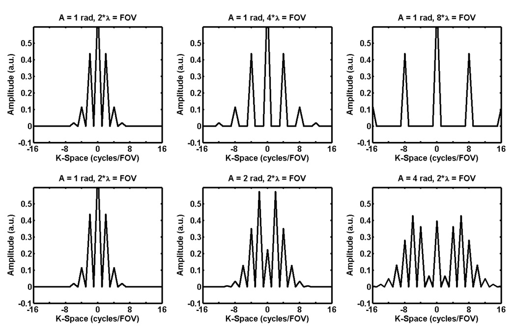
There are two important characteristics of the shear wave fields measured with MRE that affect the amount of k-space data that must be acquired: the shear wavelength and amplitude. Since shear waves in the brain tend to have a long wavelength per field of view (FOV) and low amplitude, there are significant opportunities to reduce acquisition times for brain MRE by minimizing the amount of k-space sampled. To demonstrate this point, consider a simple 1D signal with constant magnitude M (representing the magnitude of the transverse magnetization measured in MR) and a sinusoidally varying phase with a single frequency representative of a MRE-encoded shear wave with a fixed wavelength. This signal has the form M*exp(i*A*sin(2π*x/λ)), where A is the amplitude of the shear wave and λ is its spatial wavelength. Figure 1 shows the Fourier transform of this signal with varying amplitudes and wavelengths. The plots show that long-wavelength, low-amplitude MRE data have a small spectral width in k-space and thus require less sampling than short-wavelength and high-amplitude MRE data.

Figure 1.

Plots of k-space for a 1D signal with unit magnitude and sinusoidally varying phase of various amplitudes and wavelengths. The spectral width in k-space increases as the wavelength decreases and the amplitude of the phase oscillation increases.

Materials and Methods

Simulated Data

Simulated data were used to determine the effect of different sampling strategies on the accuracy of the stiffness estimates of a known subject. A 2D plane-strain finite element model (FEM) of the brain was constructed using COMSOL Multiphysics (COMSOL, Inc., Burlington, MA). The model was constructed from a human brain MRI data set which was segmented into gray matter, white matter, and cerebrospinal fluid (CSF). The gray matter, white matter and CSF regions were assigned complex shear modulus values of 4.33+1*i, 3.73+2*i kPa, and 0.1+2.34*i, respectively, with a density of 1000 kg/m³ and Poisson’s ratio equal to 0.49995. This resulted in a shear stiffness (or density times shear wave speed squared) of 4.50 kPa for all regions while creating a large attenuation coefficient in the CSF. The shear modulus data were used as a lookup table into a single-domain model with a boundary constructed to match the perimeter of the outer surface of the brain tissue in the MR image. The domain was meshed assuming a mixed U-P formulation for nearly incompressible media with 61,504 triangular Lagrange U₃P₂ elements yielding 679,203 degrees of freedom. The boundary elements were prescribed to vibrate tangentially to the surface of the brain, producing an effect similar to a rotational vibration around the center of the brain. A frequency response analysis was performed at 60 Hz. From the FEM solution, the x and y components of displacement were evaluated on a 256 × 256 grid in a 21 × 21 cm FOV with 4 time offsets and scaled to a dynamic range of 2 radians for the maximum displacement.

Wave data corresponding to the positively and negatively motion-encoded data from MRE were constructed by dividing the amplitude of the simulated data in half for the positively motion-encoded data, and assigning the negative of the positively motion-encoded data to be the negatively motion-encoded data. Simulated complex-valued MR images for each motion-encoded data set were obtained by constructing complex images with unit magnitude in the domain corresponding to the brain and with phase values equal to the positively or negatively motion-encoded phase data described above. The full k-space data for each data set were then obtained by Fourier transforming these complex-valued images. To test the effects of noise on stiffness error, normally distributed noise with zero mean was added to both the real and imaginary parts of these complex data in the image domain before performing the Fourier transform. The standard deviations of the noise were chosen such that the minimum phase SNR after wave amplitude thresholding would be 2.5, 5.0 or 7.5.

MR Data

In vivo brain MRE data were used to assess the impact of different MR sampling strategies on the elastograms for a normal, healthy volunteer. The study was performed after obtaining oral and written consent from the volunteer in accordance with the institutional review board. All data were collected on a 1.5-T MR imager (SIGNA Excite, GE Healthcare, Waukesha, WI) using an 8-channel receive-only head coil and a gradient echo pulse sequence modified to include motion-encoding gradients that were synchronized with the applied external motion. Imaging parameters included an axial FOV, FOV=21 cm, 256×256 imaging matrix, TR/TE=50/27.7 ms, right-left frequency encoding direction (x direction), and one slice with a 5-mm thickness. Shear waves were generated using two customized speakers running at 60 Hz to drive two passive drums placed under the subject’s head. The speakers were driven 180° out of phase to induce a left-to-right rocking motion of the head. Four phase offsets over one cycle of motion were collected with motion encoding in each of the x, y and z directions. The acquisition was performed twice, once with the shear wave generation system turned on (the “motion” case) and once with the shear wave generation system turned off (the “no motion” case).

Coil calibration data were also collected for the simulated SENSE acquisition and reconstruction described below. The acquisition parameters were the same as the acquisition above except that no motion-encoding gradients were applied, so the TE was only 11 ms. The shear wave generation system was off for this acquisition and only a single image was acquired (i.e., one phase offset and one encoding direction). The k-space data for the calibration images were filtered with a circular Gaussian lowpass filter with a standard deviation of 42*Δk = 2 cm⁻¹ prior to being Fourier transformed to produce smooth, high-SNR data for the SENSE reconstruction.

Data Processing

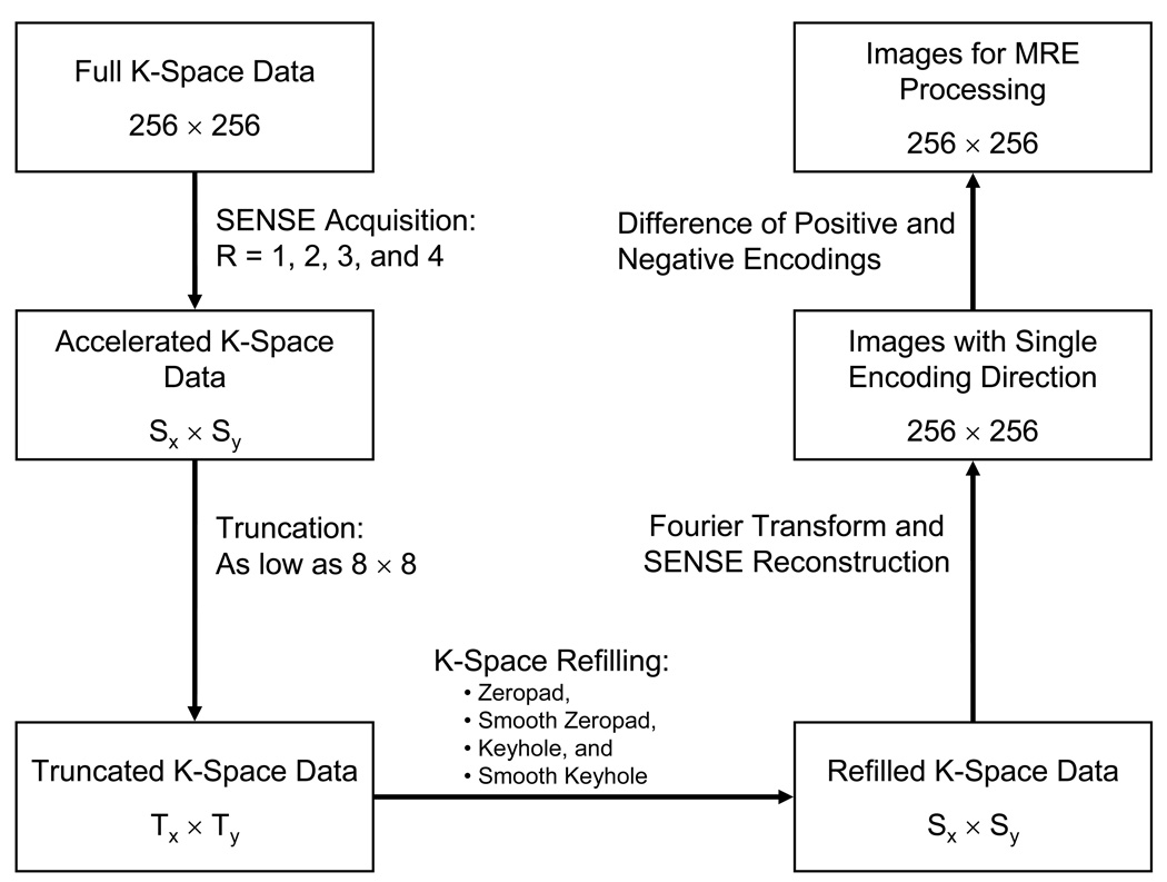
Figure 2 shows a flow diagram of the processing performed on the MRE data. The in vivo data were undersampled by a factor R to simulate a SENSE acquisition strategy with an acceleration factor of R (R = 1, 2, 3, and 4). For example, every other row of k-space was kept for R = 2 and every third row was kept for R = 3. For the FEM data, no SENSE simulation was done due to the absence of coil sensitivity data. To simulate the effects of not sampling the periphery of k-space to reduce acquisition time, the SENSE-undersampled k-space data were truncated in increments of 8 k-space samples along both the k_x and k_y directions. Thus for R = 1 each data refilling method described below was tested on 1024 new data sets (32 subsampling resolutions in each of the k_x and k_y directions) while for R = 2 each method was tested on 512 data sets (32 subsamplings in k_x and 16 subsamplings in k_y). Four strategies for restoring the truncated k-space data (“refilling”) were investigated and are outlined below: zeropadding, smooth zeropadding, keyhole, and smooth keyhole. Each truncated data set was refilled to the original size of the SENSE-undersampled data according to R (e.g., R = 1 data were filled to 256×256, R = 2 data were filled to 256×128). A SENSE reconstruction was then performed on these refilled data sets to obtain complex-valued images for the MRE processing.

Figure 2.

Flow diagram of the image processing performed to yield MRE images with various amounts of truncation and techniques for k-space refilling.

For the MRE processing, phase-difference or wave images were calculated from the positively and negatively motion-encoded images reconstructed according to Figure 2. The resulting wave images were filtered with a 4^th-order Butterworth bandpass filter with cutoff frequencies of 2.5 and 40 wavelengths/FOV (0.12 and 1.9 cm⁻¹, respectively). The two or three sets of wave images (x, y and z motion encodings) were inverted using a local frequency estimation (LFE) algorithm and combined by a weighted sum according to the amplitude of motion [21]. Stiffness measurements were averaged over a region of interest that was obtained by thresholding the phase-difference SNR (the product of phase amplitude and magnitude SNR) for the in vivo data or the phase amplitude for the FEM simulation data and excluding 10 pixels from the brain’s edge (approximately ¼ of a shear wavelength). The thresholds chosen were a phase-difference SNR greater than 5 for the in vivo data and a phase amplitude of motion greater than 0.5 radians in the simulation data. The stiffness images (elastograms) were then normalized to and compared against the stiffness calculated using the fully sampled motion data.

Data removed from k-space during truncation were refilled using four methods: zeropad, smooth zeropad, keyhole, and smooth keyhole. The zeropad method simply kept the sampled center of the k-space acquired with motion and replaced the edges of k-space with zeros. The smooth zeropad data sets were generated by lowpass filtering the central k-space collected with motion with the filter described below which smoothly goes to zero at the edges of the central k-space region. The keyhole reconstruction kept the center of the k-space collected with motion and replaced the edges of k-space with data from the same locations of the fully sampled k-space acquired without motion. Finally, the smooth keyhole data were created by adding lowpass filtered k-space of the truncated data with motion to highpass filtered k-space data without motion.

The lowpass filters used in this work in one direction had the form (1-x²)² for -1 ≤ x ;≤ 1 [22]. The filters were given a length N_x + 2, where N_x is the number of elements to keep in the x direction. The length was increased by 2 since the filter is zero at the ends where x = ±1. By increasing the length by 2, N_x represents the number of elements with a nonzero contribution after filtering. A second 1D filter was made in the y direction with length N_y + 2. The final 2D filter was calculated by taking the product of the two 1D filters. The corresponding highpass filter used for the smooth keyhole method was obtained by taking 1 minus the lowpass filter.

Minimization of Acquisition Time

The purpose of this analysis was to assess which processing methods would allow the minimum acquisition time with the smallest error in the final average stiffness measurement. The acceptable level of error in the stiffness value was set at 10% of the mean value of the original, fully sampled data and is equal to the tolerance selected by Hamhaber et al. in [4]. To select the data sets that minimized acquisition time and stiffness error, three criteria needed to be met:

1. The measured stiffness fell within 10% of the stiffness obrtained from the fully sampled data, and remained within this tolerance when additional motion data were used in the reconstruction.

2. For those data sets that satisfied the first criterion, the data set that would minimize the effective acquisition time for each of the hypothetical 2D, 3D and EPI acquisition strategies described below was selected.

3. If multiple data sets met the first acceptance criterion and shared the same acquisition time, the data set with the smallest stiffness error was selected.

Minimum acquisition times (T_acq) were determined for each of the data reduction methods for three hypothetical acquisition methods: conventional 2D imaging, isotropic 3D imaging, and 2D echo planar imaging (EPI). The acquisition times are reported in terms of the number of repetitions (NR) of a scan, or the number of shots in the case of EPI, performed with motion. NR for a 2D acquisition is just equal to the number of acquired phase encodes (N_y). NR for a 3D acquisition is N_x*N_y, where x and y are treated as the two phase encoding directions for 3D imaging. To determine the number of shots for an EPI acquisition, it was assumed that 8 ms was the maximum total readout length, with a conservative readout gradient waveform designed assuming 4 µs per sample (250 kHz bandwidth) and 144 µs per ramp with no ramp sampling.

Results

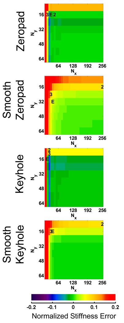
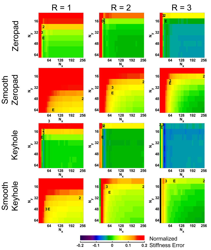
Error maps for the FEM data reconstructed using the 4 different k-space filling techniques are shown in Figure 3. The error maps represent the difference in the normalized stiffness between each subsampled data set and the fully sampled data set. The top left corner of each map indicates the error for data reconstructed with only the center 8×8 samples of the original k-space data, while the bottom right represents the error using the full 256×256 k-space data. The data set that minimized the acquisition time for each of the three hypothetical acquisition methods are indicated on the maps by “2” (2D), “3” (3D) and “E” (EPI). The error maps for the FEM data show that the zeropadding and keyhole techniques produce similar trends in the stiffness error. Increased truncation manifests as subtle ringing in the wave images, introducing artifactual high-frequency information and biasing the LFE stiffness toward lower values. This behavior is indicated by the blue bands near the edge of the error map. Even further truncation results in the removal of essential information about the shear waves, fundamentally changing the wavelength and creating invalid shear wave data. The smooth zeropadding and keyhole methods reduce this high-frequency ringing behavior and make the stiffness errors increase more monotonically with decreased sampling. Minimum acquisition times for the FEM data are listed in Table 1.

Figure 3.

Normalized error maps for each data reduction method using the FEM data. These maps are used to find subsamplings or image acquisition matrices that meet the 10% tolerance and minimize T_acq. The data set that minimized T_acq for each of the three acquisition methods is denoted by “2” (2D), “3” (3D) or “E” (EPI).

Table 1.

Number of repetitions required for each data reduction method to achieve 10% error or less using the FEM data.

Reduction Method	Acquisition Type
	2D (Ny)	3D (Nx*Ny)	EPI (Shots)
Zeropad	16	256	1
Smooth Zeropad	16	768	2
Keyhole	8	192	1
Smooth Keyhole	8	512	1

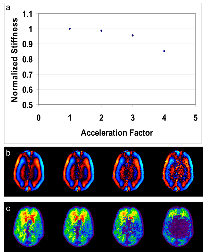
For the in vivo data, examples of the effect of SENSE acceleration are shown in Figure 4 for the case of no k-space truncation. The stiffness estimates systematically decrease as acceleration is increased, likely due to a decrease in the signal-to-noise ratio (SNR). Since the R=4 reconstruction no longer meets the 10% error criterion even without k-space truncation, all remaining results shown will focus on the cases of R=1, 2 and 3.

Figure 4.

In vivo brain MRE data simulated with 4 different SENSE acceleration factors. (a) A plot of normalized mean stiffness versus acceleration factor with no k-space truncation. Example wave images (b) and elastograms (c) obtained with R = 1, 2, 3, and 4 show how the stiffness decreases with increasing acceleration, likely due to the decrease in SNR.

Error maps for the in vivo MR data reconstructed with SENSE acceleration factors of 1, 2 and 3 are shown in Figure 5. These maps look qualitatively different from the FEM simulation error maps. Most notably, the zeropad results for R=1 indicate a progressively increasing stiffness as the k-space data are increasingly truncated. The keyhole results are more similar to the FEM results, indicating a decrease in stiffness until very severe levels of data truncation are reached at the very edge of the error map. The minimum acquisition times for these simulations are listed in Table 2. This table indicates that the keyhole technique required less k-space data (512 points for R=1) than the zeropad method (768 points). The results imply that for MR data, keyhole can save a significant amount time, particularly for a 3D acquisition. The results involving a SENSE acceleration as high as 3 indicate even greater time efficiency, however the cost is an initial amount of intrinsic error due to the acceleration.

Figure 5.

Normalized error maps for each data reduction method using the in vivo MR data. These maps are used to find subsamplings or image acquisition matrices that meet the 10% tolerance and minimize T_acq. The data set that minimized T_acq for each of the three acquisition methods is denoted by a “2” (2D), “3” (3D) or “E” (EPI).

Table 2.

Number of repetitions required for each data reduction method to achieve 10% error or less using the in vivo MR data.

Acceleration Factor	Reduction Method	Acquisition Type
		2D (Ny)	3D (Nx*Ny)	EPI (Shots)
R = 1	Zeropad	24	768	2
	Smooth Zeropad	48	5120	7
	Keyhole	16	512	1
	Smooth Keyhole	32	2304	4
R = 2	Zeropad	16	384	1
	Smooth Zeropad	24	2560	4
	Keyhole	8	192	1
	Smooth Keyhole	16	768	2
R = 3	Zeropad	8	192	1
	Smooth Zeropad	16	1536	2
	Keyhole	8	128	1
	Smooth Keyhole	8	320	1

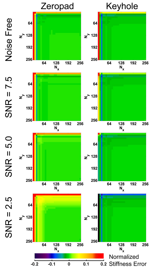
To test the hypothesis that the differences in the behavior of the FEM and in vivo data are due to noise, noise with varying standard deviations was added to the FEM data to produce data with minimum phase SNRs of 2.5, 5.0 and 7.5. Only zeropad and keyhole filling methods were used in these reconstructions and the resulting error maps are shown in Figure 6. Each of the four data sets with different noise levels was normalized to its own fully sampled data set to mimic the in vivo data where the experimenter does not have access to the noise free case. These maps show that as noise is added to the FEM data, the trends in error approach the same trends seen in the in vivo data. For the case of SNR = 2.5, the FEM zeropad error map looks similar to the in vivo zeropad error map; stiffness estimates increase as data truncation increases. Meanwhile, the keyhole method replaces the removed noise with similarly noisy data from the no motion data. As a result, the keyhole method maintains the SNR of the fully sampled data and, along with it, the slightly negative bias in the LFE stiffness due to the presence of high-frequency noise. It is this maintenance of SNR that allows keyholed data to be truncated further than the zeropadded data when compared to fully sampled data.

Figure 6.

Error maps for the zeropad and keyhole data reduction methods using the FEM simulation data with varying SNR normalized to the stiffness obtained with fully sampled data containing the same noise. These maps demonstrate that the addition of noise produces similar trends in error in simulated data as is seen in the in vivo data.

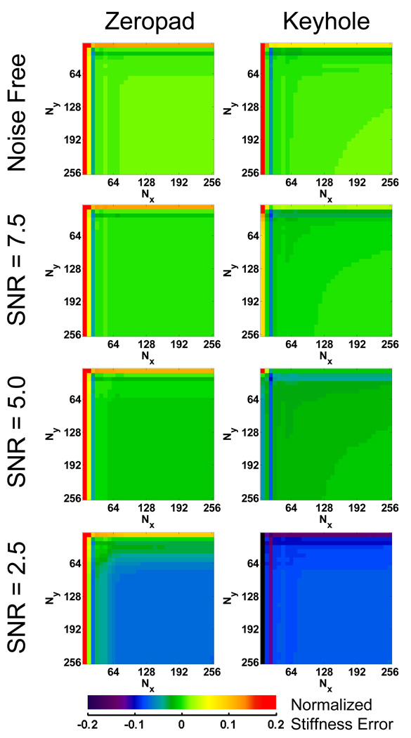
However, for the FEM data, the error maps can also be normalized to the true stiffness and those maps are shown in Figure 7. At the highest noise level, SNR = 2.5, the zeropad and keyhole error maps both contain a large blue plateau in the lower right, indicating that the fully sampled data actually produces an underestimate of the true stiffness in the presence of noise The difference between the two methods becomes evident in the upper left portion of the maps where truncation is more significant. Keyhole methods result in low stiffness estimates (purple bands), while the zeropad results start to increase (green band) and approach the true stiffness.

Figure 7.

Error maps for the zeropad and keyhole data reduction methods using the FEM simulation data with varying SNR normalized to the true stiffness. Noise biases the inversion toward a lower stiffness, but an increase in SNR due to truncation and zeropadding alleviates this bias.

Discussion

The results of this study suggest that a significant reduction in acquisition time can be achieved for brain MRE acquisitions while maintaining an error in the mean brain tissue stiffness comparable to variations observed in typical reproducibility studies of MRE stiffness.

Inspection of the zeropadded FEM data results indicates the small spectral width of k-space data that mimic brain MRE data. There is a large plateau in the error map, illustrating that a significant amount of data can be removed with minimal impact on the inversion results. The stiffness estimates then begin to drop as ringing arises in the wave images creating artifactual high-frequency information. The keyhole method follows a similar trend but with larger error at the highest levels of truncation.

The noisy MR data behaved differently than the simulated data. Zeropadding MR data causes the stiffness measurements to increase because noise is being filtered out due to the k-space truncation, removing high-frequency energy that can lower the LFE stiffness estimate. On the other hand, using a keyhole method maintains the noise characteristics found in the fully sampled data, resulting in stiffness estimates that agree better with the original fully sampled data. While the keyhole method does allow for the most truncation of the data by the criteria set earlier, it only accomplishes this by reintroducing a bias due to noise present in the fully sampled data. Therefore, zeropadding is a better approach for reducing acquisition time while also maintaining accuracy in the stiffness estimate.

The use of a windowing function did not improve the performance for the zeropad or keyhole techniques in this study. While simply truncating the k-space data is a poor filter design strategy, it still resulted in less error than using a smooth windowing function of the same length because the windowing function further smooths the data and biases the stiffness toward higher values. The stiffness measurements in this study systematically dropped as the SENSE acceleration factor was increased. This trend was the result of decreasing SNR, which biases the inversion toward decreased stiffness. However an acceleration factor of 3 was still acceptable and within the criterion of 10% error while providing additional time savings.

For a conventional 2D pulse sequence, the results from this study indicate that the optimal acquisition protocol for brain MRE is with a SENSE acceleration factor of 3 with N_y of only 8. The results further indicate that the optimal isotropic 3D acquisition would use R=3 with a 24×8 imaging matrix and zeropad data filling. A true 3D Fourier acquisition does not seem necessary for a full brain stiffness measurement, compared to conventional 2D multislice imaging, since this work indicates a relatively low resolution is required for brain MRE (a resolution that can be obtained by standard slice-selective excitations). However, a 3D pulse sequence may be useful for collecting several thin slices of data over a small structure of interest to apply a 3D inversion algorithm. The most efficient simulated EPI acquisition in this work was with R=2 with a prescribed imaging matrix of 32×16 and zeropad data filling. This amount of data can be collected in a single shot. Since this can already be collected in a single shot, it is preferred over a method with R=3 to maximize SNR.

In conclusion, this work shows that whole-slice brain MRE data at frequencies on the order of 60 Hz can be acquired with very low resolution while still maintaining acceptable levels of error in the reconstructed elastograms. In fact, the simulation data indicate that low-resolution MRE data may provide more accurate global brain stiffness estimates than high-resolution data by improving SNR. The extent of k-space needed to maintain less than 10% error can be acquired in just 8 lines for a 2D acquisition or can easily be covered with a single-shot EPI acquisition. These results, however, may not hold for other tissues, driving frequencies, processing methods or regions of interest. Each application of MRE needs a similar analysis to determine how to minimize its acquisition time. These data show the merit in attempting to use fast brain MRE protocols in future studies designed to diagnose diffuse diseases that may alter brain tissue mechanical properties.

References

- 1.Muthupillai R, Lomas DJ, Rossman PJ, Greenleaf JF, Manduca A, Ehman RL. Magnetic resonance elastography by direct visualization of propagating acoustic shear waves. Science. 1995;269(5232):1854–1857. doi: 10.1126/science.7569924. [DOI] [PubMed] [Google Scholar]
- 2.Atay SM, Kroenke CD, Sabet A, Bayly PV. Measurement of the Dynamic Shear Modulus of Mouse Brain Tissue In Vivo by Magnetic Resonance Elastography. J Biomech Eng. 2008;130(2):021013. doi: 10.1115/1.2899575. [DOI] [PMC free article] [PubMed] [Google Scholar]
- 3.Green MA, Bilston LE, Sinkus R. In vivo brain viscoelastic properties measured by magnetic resonance elastography. NMR Biomed. 2008;21:755–764. doi: 10.1002/nbm.1254. [DOI] [PubMed] [Google Scholar]
- 4.Hamhaber U, Sack I, Papazoglou S, Rump J, Klatt D, Braun J. Three-dimensional analysis of shear wave propagation observed by in vivo magnetic resonance elastography of the brain. Acta Biomater. 2007;3:127–137. doi: 10.1016/j.actbio.2006.08.007. [DOI] [PubMed] [Google Scholar]
- 5.Klatt D, Hamhaber U, Asbach P, Braun J, Sack I. Noninvasive assessment of the rheological behavior of human organs using multifrequency MR elastography: a study of brain and liver viscoelasticity. Phys Med Biol. 2007;52:7281–7294. doi: 10.1088/0031-9155/52/24/006. [DOI] [PubMed] [Google Scholar]
- 6.Kruse SA, Rose GH, Glaser KJ, Manduca A, Felmlee JP, Jack CR, Jr, Ehman RL. Magnetic Resonance Elastography of the Brain. Neuroimage. 2008;39(1):231–237. doi: 10.1016/j.neuroimage.2007.08.030. [DOI] [PMC free article] [PubMed] [Google Scholar]
- 7.McCracken PJ, Manduca A, Felmlee JP, Ehman RL. Mechanical transient-based magnetic resonance elastography. Magn Reson Med. 2005;53(3):628–639. doi: 10.1002/mrm.20388. [DOI] [PubMed] [Google Scholar]
- 8.Sack I, Beierbach B, Hamhaber U, Klatt D, Braun J. Non-invasive measurement of brain viscoelasticity using magnetic resonance elastography. NMR Biomed. 2008;21:265–271. doi: 10.1002/nbm.1189. [DOI] [PubMed] [Google Scholar]
- 9.Sack I, Beierbach B, Wuerfel J, Klatt D, Hamhaber U, Papazoglu S, Martus P, Braun J. The impact of aging and gender on brain viscoelasticity. Neuroimage. 2009;46(3):652–657. doi: 10.1016/j.neuroimage.2009.02.040. [DOI] [PubMed] [Google Scholar]
- 10.Vappou J, Breton E, Choquet P, Goetz C, Willinger R, Constantinesco A. Magnetic resonance elastography compared with rotational rheometry for in vitro brain tissue viscoelasticity measurement. MAGMA. 2007;20:270–278. doi: 10.1007/s10334-007-0098-7. [DOI] [PubMed] [Google Scholar]
- 11.Vappou J, Breton E, Choquet P, Goetz C, Willinger R, Constantinesco A. Assessment of in vivo and post-mortem mechanical behavior of brain tissue using magnetic resonance elastography. J Biomech. 2008;41(14):2954–2959. doi: 10.1016/j.jbiomech.2008.07.034. [DOI] [PubMed] [Google Scholar]
- 12.Wuerfel J, Paul F, Beierbach B, Hamhaber U, Klatt D, Papazoglou S, Zipp F, Martus P, Braun J, Sack I. MR-elastography reveals degradation of tissue integrity in multiple sclerosis. Neuroimage. 2009 doi: 10.1016/j.neuroimage.2009.06.018. [DOI] [PubMed] [Google Scholar]
- 13.Xu L, Lin Y, Xi ZN, Shen H, Gao PY. Magnetic Resonance Elastography of the Human Brain: A Preliminary Study. Acta radiol. 2007;48(1):112–115. doi: 10.1080/02841850601026401. [DOI] [PubMed] [Google Scholar]
- 14.Xu L, Lin Y, Han JC, Xi JN, Shen H, Gao PY. Magnetic Resonance Elastography of Brain Tumors: Preliminary Results. Acta radiol. 2007;48(3):327–330. doi: 10.1080/02841850701199967. [DOI] [PubMed] [Google Scholar]
- 15.Hardy J, Selkoe DJ. The Amyloid Hypothesis of Alzheimer's Disease: Progress and Problems on the Road to Therapeutics. Science. 2002;297:353–356. doi: 10.1126/science.1072994. [DOI] [PubMed] [Google Scholar]
- 16.Meyer E, Ulmann-Schuler A, Staufenbiel M, Krucker T. Altered morphology and 3D architecture of brain vasculature in a mouse model for Alzheimer's disease. Proc Natl Acad Sci U S A. 2008;105(9):3587–3592. doi: 10.1073/pnas.0709788105. [DOI] [PMC free article] [PubMed] [Google Scholar]
- 17.Bjartmar C, Kinkel RP, Kidd G, Rudick RA, Trapp BD. Axonal loss in normal-appearing whit matter in a patient with acute MS. Neurology. 2001;57(7):1248–1252. doi: 10.1212/wnl.57.7.1248. [DOI] [PubMed] [Google Scholar]
- 18.Adams R, Fisher CM, Hakim S, Ojemann RG, Sweet WH. Symptomatic occult hydrocephalus with "normal" cerbrospinal fluid pressure: A treatable syndrome. N Engl J Med. 1965;273:116–126. doi: 10.1056/NEJM196507152730301. [DOI] [PubMed] [Google Scholar]
- 19.Hebb A, Cusimano MD. Idiopathic Normal Pressure Hydrocephalus: A Systematic Review of Diagnosis and Outcome. Neurosurgery. 2001;49(5):1166–1186. doi: 10.1097/00006123-200111000-00028. [DOI] [PubMed] [Google Scholar]
- 20.Geschwind N. The mechanism of normal pressure hydrocephalus. J Neurol Sci. 1968;7(3):481–493. doi: 10.1016/0022-510x(68)90054-3. [DOI] [PubMed] [Google Scholar]
- 21.Manduca A, Oliphant TE, Dresner MA, Mahowald JL, Kruse SA, Amromin E, Felmlee JP, Greenleaf JF, Ehman RL. Magnetic resonance elastography: Non-invasive mapping of tissue elasticity. Med Image Anal. 2001;5:237–254. doi: 10.1016/s1361-8415(00)00039-6. [DOI] [PubMed] [Google Scholar]
- 22.Romano AJ, Bucaro JA, Ehman RL, Shirron JL. Evaluation of a Material Parameter Extraction Algorithm Using MRI-Based Displacement Measurements. IEEE Trans Ultrason Ferroelectr Freq Control. 2000;47(6):1575–1581. doi: 10.1109/58.883546. [DOI] [PubMed] [Google Scholar]