Robust Deformable Image Registration using Prior Shape Information for Atlas to Patient Registration

Abstract

Statistical atlases enable the individualization of atlas information for patient specific applications such as surgical planning. In this paper, a statistical atlas comprising a point distribution model defined on the vertices of a tetrahedral mesh is registered to a subject’s computed tomography scan of the human pelvis. The approach consists of a volumetric deformable registration method augmented to maintain the topology of the atlas mesh after deformation as well as incorporating the dominant three-dimensional shape modes in the atlas. Experimental results demonstrate that incorporation of the statistical shape atlas helps to stabilize the registration and improves robustness and registration accuracy.

1 Introduction

The creation and use of statistical atlases in scientific inquiry and medical applications has increased dramatically in recent years [1–4]. Atlases have been commonly used to learn about shape variation in anatomical structures and thereby contribute to the characterization of longitudinal changes in disease, growth, or aging, as well as to characterize cross-sectional differences between populations—e.g., normal versus diseased. They have also been used to hold labels that are to be transferred to a patient’s image in order to inform a diagnosis or plan therapy. In this case, the atlas statistics—e.g., shape and density variations—may be of great use in accurately registering stored atlas information to the subject. In this paper, we use shape information contained within a three-dimensional (3D) statistical atlas to inform the registration of the atlas to a subject.

Statistical models of shape have been most commonly constructed using point distribution models (PDMs) to characterize the shape variations that are present in curves in 2D or surfaces in 3D [5–7]. In such cases, variants of the active shape models are typically used to register an atlas to a given subject [8]. In this work, we are concerned with a three-dimensional statistical atlas of the human male pelvis, conceptually similar to that proposed by Yao and Taylor [1] and also described in [9]. It comprises a tetrahedral mesh whose vertex positions are described by a PDM and whose CT densities are characterized by the coefficients of Bernstein polynomials. With the registration of many subjects, principal component analysis (PCA) [6] can be computed on both shape and density variations, and the dominant modes of variations can be learned and used.

The specific task being addressed in this paper is the segmentation of the pelvis from CT data. While low level segmentation methods can be used, extraneous and highly variable details within these images, including the presence of barium contrast in the bowel, the presence of and the variable positions of the femurs, and the variation in CT table positioning, can make this task difficult, ultimately requiring human monitoring and intervention. High level segmentation, such as the “segmentation-by-registration” process described herein, requires information that guides the process in order to make it robust to these extraneous influences but should not be so constraining that detail is missed and fidelity lost. In our approach, the use of an atlas helps to provide the required robustness to extraneous features while the use of strong image features guarantees faithfulness to the subject’s data.

The method presented in this paper, which we refer to as Mjolnir+, is an extension of the volumetric deformable registration method called Mjolnir [10], which in turn was modeled after the registration method HAMMER [11]. In particular, we augmented Mjolnir both to incorporate the dominant 3D shape modes in the statistical atlas and to maintain the topology of the atlas mesh after deformation. In extensive experiments, we demonstrate that these extensions can significantly enhance algorithm robustness, yielding a pelvis segmentation result that is consistently reliable and accurate in CT data having highly variable characteristics and overall quality.

2 Statistical Atlas

We are concerned with a 3D statistical atlas of the human male pelvis comprising two features: 1) a model tetrahedral mesh $\overline{\mathrm{ℳ}}$ having N_V vertices and N_T tetrahedra describing the shape of the mesh, and 2) CT densities which give its likely appearance within a CT image. These characteristics are illustrated in Fig. 1. For convenience in describing statistical variation of shape, the positions of the mesh vertices are stacked in a vector 𝐦̅ ∈ ℝ^V, where V = 3N_V. The actual 3D position of the i-th vertex is given by 𝐯̄_i = (m̄_i, m̄_i+NV, m̄_i+2NV) ∈ ℝ³, where m̄_i is the i-th element of 𝐦̅. The CT densities are defined on the model tetrahedra by specifying coefficients of Bernstein polynomials on the barycentric grid defined by the vertices, as described in [1]. In this version of the atlas, only shape is characterized by statistical variation; the CT densities are assumed to be constant and known.

Fig. 1.

(a) A 3D rendering of the tetrahedral mesh representation of the atlas. (b) A 2D slice from the 3D density image.

The statistical atlas was constructed according to standard procedures in principal component analysis (PCA) of shapes (see [6]) from 41 normal male pelvis CT scans. One CT scan was randomly selected to serve as a template pelvis. The pelvic bone of this image was manually segmented and a 3D tetrahedral mesh ${\mathrm{ℳ}}_0$, comprising 26875 vertices and 105767 tetrahedra, created from the segmentation using the method by Mohamed and Davatzikos [12]. The remaining 40 CT scans were deformably registered to the template pelvis using Mjolnir [10], modified to register pelvis CT images and augmented to deform and preserve the topology of the template mesh (as described in Sections 5 and 6 below). This procedure provided topologically correct mesh instances ${\mathrm{ℳ}}_i$, i = 1, …, 40, for each subject, thereby deriving 26875 corresponding landmarks between each scan and the template pelvis (see details in [9]). After PCA analysis, the first M principal modes of variation (where M = 15 in our experiments) were arranged in a V (= 3 × 26875) by M matrix Φ_M = [φ₁ φ₂ … φ_M], from which a shape instance can be generated according to

$$\mathbf{m}\approx \overline{\mathbf{m}}+{\mathbf{\Phi }}_M\mathbf{b},$$ (1)

by choosing mode weights b ∈ ℝ^M [13]. During the execution of Mjolnir+, we iteratively search for b that yields a shape instance from the atlas that best matches the actual subject shape. The displacements m − 𝐦̅ defined on the model shape then provide guidance that allows Mjolnir+ to robustly and accurately bring the atlas and subject into alignment (see Section 4).

In order to analyze the size of the population and the number of principal modes needed to extract stable statistics, we randomly selected n meshes, where n = 20, 30, …, 80, and created statistical atlases using these datasets. This process was repeated 20 times for each value of n. After registering the atlas to multiple leave-out subjects (yielding “true shapes”) and estimating the given subjects using the atlas modes, we computed the vertex to vertex correspondence error between the estimated shapes and the true shapes. We then computed the average residual vertex correspondence error for each of the atlas sizes as a function of number of modes. This analysis revealed that around 40 to 50 datasets are sufficient to capture the shape variations of a healthy pelvis anatomy using 15 modes. Adding more instances to the atlas database resulted in a very small improvement, less than 0.1mm, in terms of residual errors (see details in Chintalapani et al. [9]).

3 Key Concepts

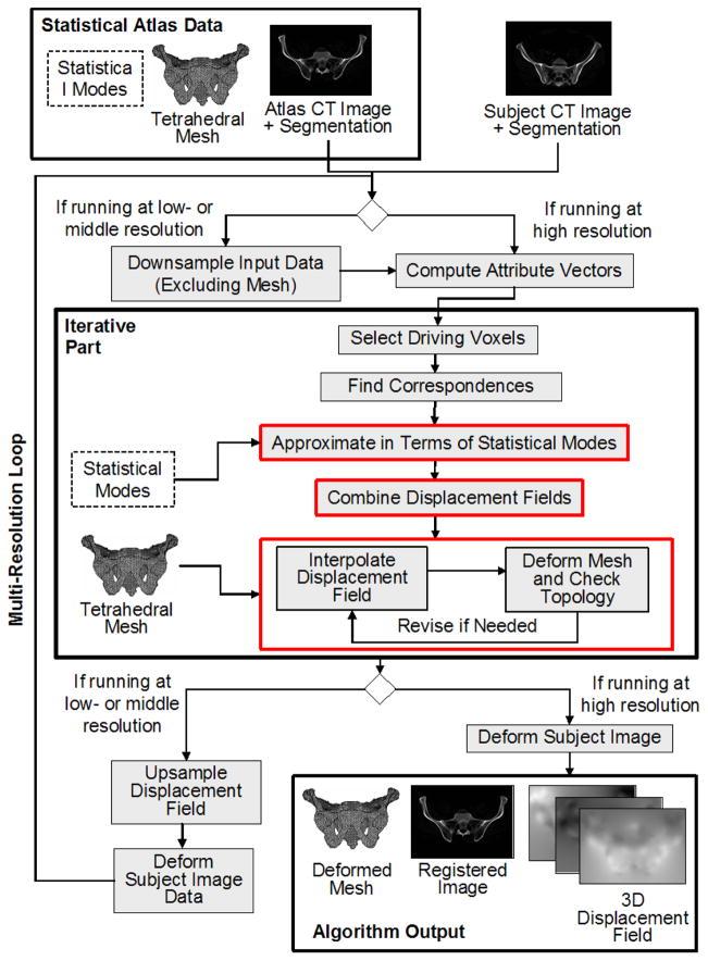
The 3D-3D deformable registration approach presented in this work, referred to as Mjolnir+, is based on a method called Mjolnir (see [10, 14] and [11]). In this section, we review the key concepts that are largely in common between these methods and also highlight certain differences that are used to take advantage of the presence of the statistical atlas in Mjolnir+. For further details about those processing steps that are in common between these methods, the reader is referred to [11] and [14]. A block diagram of Mjolnir+ is provided in Fig. 2.

Fig. 2.

Flow chart of Mjolnir+ registration technique.

Attribute Vectors

The goal of the registration algorithm is to spatially align atlas and subject images. In order for this alignment to be accurate and anatomically correct one must identify correct anatomical correspondence between the two images. Several geometric moment invariants (GMIs) are computed at a small neighborhood around each voxel in both images. These moments describe the intensity “shape” near each voxel. The CT intensity and the edge, derived from the classification of the pelvis CT image into soft tissue, trabecular bone, or cortical bone (see Section 6) are also used as features to be matched. All these pieces of information about each voxel are organized into attribute vectors, one for each voxel. This information will figure into the image similarity after registration. This procedure is done at three resolutions of each CT image—coarse, medium, and fine—and the subsequent steps are performed in sequence from coarse to fine.

Driving Voxels

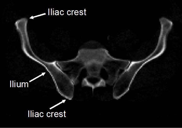
During the execution of Mjolnir+, a collection of driving voxels from both atlas and subject are determined. These are distinctive voxels in one image—as determined by their attribute vectors—that can be associated with similar points in the other image creating temporary landmark pairs that “drive” the deformation of one image toward the other. Driving voxels are “active” while all other voxels are “passive” because the displacement field at each iteration is determined solely by the displacements that are estimated at driving voxels. In Mjolnir, driving voxels are automatically selected in a hierarchical fashion, starting with a small initial set of highly distinctive voxels in both the atlas and the subject images. In Mjolnir+, the initial set of driving voxels comprises a small collection of highly distinctive voxels residing on mesh vertices rounded to the nearest voxel; these voxels are mostly located on high curvature points on the pelvic bone like the iliac crests (see Fig. 3).

Fig. 3.

The figure shows the ilium of the pelvic bone. Most of the primary driving voxels are located on the iliac crests.

In later iterations, Mjolnir+ augments the driving voxels in two ways. First, voxels in the immediate 6-neighborhood of existing driving voxels are added; in this way, the registration of edges and corners are made more precise over increasing neighborhoods around original and added driving voxels. Second, new driving voxels from increasingly less distinctive points on the mesh—i.e. voxel points near mesh vertices—are added; in this way, the influence of the image attributes on and near the mesh continues to demonstrate high influence on the registration process. Highly distinctive points within the subject image are also selected as driving voxels. In this way, important points in the subject that should play a major role in registration are also incorporated in the registration process. In each iteration, the subject image is deformed relative to the atlas image, and new driving voxels are identified in order to continue to bring the images into alignment. Various thresholds are changed throughout the registration process such that all voxels in the atlas image —and hence, all vertices rounded to the nearest voxel — eventually become driving voxels. For computational savings, the driving voxels in the subject image are never augmented to include more than just the original selection.

Correspondences

For each driving voxel in the subject and atlas images, a corresponding voxel in the other image is found, creating a (temporary) landmark pair. This is performed by searching in the opposite image for voxels with strongly similar attribute vectors. The search is performed in a spherical neighborhood around each driving voxel. The radius of the neighborhood is large in the beginning when the subject and atlas are far apart and gradually decreases to a singe voxel as the image alignment converges.

Displacement Field

After searching and finding correspondences for all driving voxels, including those located on vertices, displacement vectors pointing from the atlas to the subject are formed for each driving voxel, forming a sparse displacement field u_c(x) for each voxel position x in the domain of the atlas. This field is then interpolated and smoothed throughout the entire image domain in order to generate a dense displacement field, which yields a transformation that can be used to align the two images by warping their coordinate systems. In Mjolnir+, we regularize the displacement field u_c using prior shape information from the statistical atlas and then carry out interpolation and smoothing as in conventional Mjolnir while also preserving mesh topology. This new process is described next.

Multi-resolution scheme

The algorithm is run at three different resolutions, i.e. low, medium, and high (see Fig. 2). At low resolution, the images are downsampled by a factor four and the algorithm is run until convergence. Then the displacement field is upsampled, the subject image deformed accordingly, and the algorithm is run again at a middle resolution. This procedure is repeated once more at high resolution (i.e., the resolution of the input images).

4 Incorporating Statistical Shape Information

Mjolnir determines its correspondences based on the similarity of automatically selected driving voxels where voxel similarity is based on locally derived image features. When a CT image contains pelvic bone in the presence of non-pelvic features—e.g. femur—there is a possibility that non-homologous landmarks will be paired. Our objective is to make the registration more robust by incorporating the statistical shape modes from the atlas. This will guide the volumetric 3D-3D registration process by providing it with information on valid deformations within the atlas population, thereby preventing large, erroneous displacements from occurring.

Given the sparse displacement field u_c(x), we construct a V -dimensional vector d_m comprising the displacement vectors at voxel locations that coincide with model mesh vertices. If not regularized in any way, then the present result posits that the vertices of the model mesh should move to the positions defined by m = 𝐦̅+d_m in the subject. In order to regularize this displacement, we ask what shape in the statistical atlas is closest to this motion? This question is answered by finding the mode weights b′ that solve Φb′ = d_m in the least squares sense, which is given by

$${\mathbf{b}}^{\prime }={\mathbf{\Phi }}^T{\mathbf{d}}_m,$$ (2)

since the shape modes are orthonormal. Some of these mode weights might be very large in comparison to the expected level of variation in that mode, as determined by the PCA analysis of shape [13]. We address this by limiting each element $b_i^{\prime }$ to $\pm 3\sqrt{{\sigma }_i^2}$, where ${\sigma }_i^2$ is the variance of mode i, yielding b̃′. The regularized displacement vectors are therefore given by

$${\mathbf{d}}_m^{\prime }=\mathbf{\Phi }{\stackrel{\sim }{\mathbf{b}}}^{\prime },$$ (3)

which represents a “valid” shape as far as the atlas is concerned.

The sparse displacement field u_c(x) is then updated by combining d_m with the regularized displacements ${\mathbf{d}}_m^{\prime }$ as follows

$${\mathbf{u}}_c^{\prime }(\mathbf{x})=\{\begin{array}{ll}\alpha S_i{\mathbf{d}}_m^{\prime }+(1-\alpha )S_i{\mathbf{d}}_m,\hfill & \text{if}\mathbf{x}\text{is}\text{a}\text{driving}\text{voxel}\text{coinciding}\text{with}\text{the}i-\text{th}\text{mesh}\text{vertex},\hfill \\ {\mathbf{u}}_c(\mathbf{x})\hfill & \text{otherwise},\hfill \end{array}$$ (4)

where S_id_m = (d_m,i, d_m,i+NV, d_m,i+2NV) ∈ ℝ³ is the 3D displacement vector associated with the i-th model vertex, i = 1, …, N_V, and $S_i{\mathbf{d}}_m^{\prime }$ is similarly defined. The parameter α in (4) controls how strong the regularization should be. We set α = 1 early in the registration process, when the subject and atlas are far apart, and linearly decrease it to 0 as the subject and atlas converge—i.e., α = 1 − τ, where τ = k/maxIter, k is the current iteration, and maxIter is the maximum number of iterations.

During the early stages of the algorithm, most driving voxels come from the atlas mesh vertices and the displacement field ${\mathbf{u}}_c^{\prime }$ is strongly determined by the first condition in (4). Since α ≈ 1 at this stage, the atlas has a dominant influence on the computed deformation. Later, as driving voxels are gradually extended to include all voxels, the influence of the atlas becomes negligible, and local image features dominate the final registration result.

5 Preserving Mesh Topology

In order to determine a dense displacement field throughout the entire image domain, the atlas-regularized sparse displacement field ${\mathbf{u}}_c^{\prime }(\mathbf{x})$ must be interpolated. Mjolnir estimates a dense field u(x) using the following partial differential equation (PDE) [14]

$$g{\nabla }^2\mathbf{u}(\mathbf{x})-p(\mathbf{x})(\mathbf{u}(\mathbf{x})-{\mathbf{u}}_c^{\prime })=\mathbf{0},$$ (5)

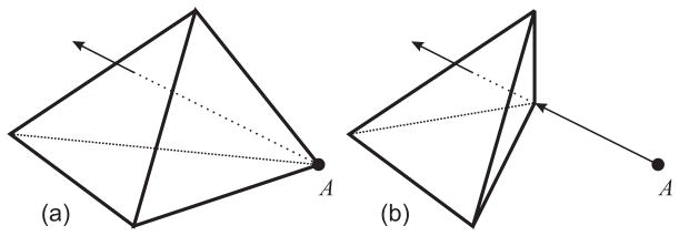
where ∇² = ∂²/∂x² + ∂²/∂y² + ∂²/∂z² is the Laplacian operator, g is a scalar weight, and p is a weight function (see [14] for specifics). This equation yields a smooth field in regions in which no driving voxels exist and adheres to the displacements at the existing driving voxels (modulated by the similarity of the underlying images at the regions matched by the driving voxels). In Mjolnir+, we must consider the fact that the resultant field does not guarantee that the tetrahedral mesh in the atlas will warp into a valid tetrahedral mesh in the subject. For example, it is possible that tetrahedra could “flip” from positive volumes to negative volumes, which cannot be allowed because this corresponds to an invalid atlas instance, i.e., an invalid object topology, as shown in Fig. 4(a).

Fig. 4.

(a) Invalid displacement of a vertex causes it to “punch” through the opposite face of the tetrahedron. (b) A reduced displacement that maintains the topology of the tetrahedron after deformation.

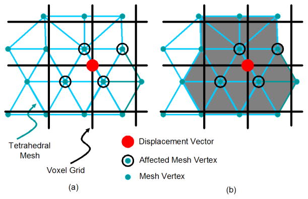
In order to preserve the object topology, the sign of the volume of each tetrahedron in the atlas mesh is monitored during the registration process. As shown in Fig. 2, after u(x) is computed using (5), we visit each voxel position x_l and look for mesh vertices residing in the vicinity of x_l. Such vertices will be affected by the displacement vector w_l = u(x_l) as their displacements will be interpolated using w_l. This is demonstrated in Fig. 5(a). We compute the volumes of each tetrahedron whose vertex is in the vicinity of x_l, as illustrated in Fig. 5(b), and if any volume is less than 0.1 mm³ then the displacement is deemed to be invalid. The displacement vector w_l causing this problem is therefore reduced in length, as shown in Fig. 4(b), until the volumes of all affected tetrahedra in the vicinity of the displacement vector are greater than or equal to 0.1 mm³. This process is described in detail in Algorithm 1 below.

Fig. 5.

(a) Affected vertices (black circles) when the displacement vector at the voxel marked with a red dot is modified. (b) The volumes of the gray tetrahedra need to be checked to see if the displacement at the red dot will affect their topology.

Algorithm 1 (Topology Preservation)

Given the topologically correct displacement field u^k−1 computed at the previous iteration of Mjolnir+ and given the displacement field u computed using Eqn. (5), we compute the topologically correct displacement field u^k as follows:

1. Initialize the revised displacement field as ũ = u^k−1.

2. Initialize the vector of revised vertex positions as ṽ_i = 𝐯̄_i + u^k−1(𝐯̄_i), i = 1, …, N_v.

3. For each voxel position x_l do the following:

   1. Compute the current displacement contribution at x_l as ${\mathbf{w}}_l^0=\mathbf{u}({\mathbf{x}}_l)-{\mathbf{u}}^{k-1}({\mathbf{x}}_l)$. Update ũ(x_l) = u(x_l).

   2. Check if there is a mesh vertex 𝐯̄_j in the vicinity of x_l that will be affected by this displacement vector, i.e., check if |𝐯̄_j − x_l| < 1 voxel.

   3. Set iteration counter i = 0.

   4. For each affected vertex 𝐯̄_j, update its position in the mesh as ṽ_j = 𝐯̄_j + ũ(𝐯̄_j).

   5. For each affected tetrahedron—i.e. a tetrahedron that has 𝐯̄_j as its vertex—compute its volume (using the just updated vertex positions).

      1. If the volumes are all greater than 0.1 mm³, go to step 3a and look at the next voxel and corresponding displacement vector.

      2. Else if the number of iterations i has reached 100, set ũ(x_l) = u^k−1(x_l). Update each affected vertex as ṽ_j = 𝐯̄_j + ũ(𝐯̄_j). Go to step 3a and look at the next voxel and corresponding displacement vector.

      3. Else for each tetrahedron with a negative volume, decrease the displacement vector that caused the flip: ${\mathbf{w}}_l^{i+1}=0.9\times {\mathbf{w}}_l^i$. Update $\stackrel{\sim }{\mathbf{u}}({\mathbf{x}}_l)={\mathbf{u}}^{k-1}({\mathbf{x}}_l)+{\mathbf{w}}_l^{i+1}$. Increment i = i + 1 and go to step 3d.

4. Check the topology of the revised mesh. If the topology is correct, set u^k = ũ. Otherwise, go to step 2 and iterate through the algorithm again until no more tetrahedra with negative volumes exist.

Algorithm 1 is guaranteed to converge since in the limit, the displacement field goes all the way back to the previous configuration—i.e., from the previous iteration—in which case Algorithm 1 ends.

6 Input Data and Preprocessing

Mjolnir+ is specifically tuned for the registration of CT images of the human pelvis to a statistical atlas comprising a tetrahedral mesh whose vertex positions are described by a PDM, a CT image representation, and statistical modes of shape variation described by displacement matrices. Very few (if any) modifications need to take place in order to utilize the method to register other bony structures from CT images such as femur, as long as the atlas data structure is as described above.

The foundation of the registration algorithm is the alignment of a CT image coming from a patient to the density image of the atlas shown in Fig. 1(b). The atlas density image contains information about the pelvic bone but not the soft tissue surrounding the pelvis, such as fat or muscles. In order to make the patient CT image more comparable with the atlas density image, a simple preprocessing step is performed on the patient CT data to “remove” the soft tissue from the image, as demonstrated in Fig. 6.

Fig. 6.

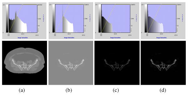
Demonstration of the preprocessing step performed on the patient’s CT data to make it more comparable with the atlas density image. The top row shows intensity histograms corresponding to the figures in the bottom row. (a) Original image. (b) Intensities below bone CT densities set to typical soft tissue values. (c) Intensities shifted such that the background is set to zero. (d) Intensities normalized.

Fig. 6(a) shows a patient CT image (bottom) and the corresponding intensity histogram (top). We can select a typical soft tissue value (determined as the average intensity over a selected soft tissue region) that works for all patient CT scans of the pelvis since CT intensities are in general standardized in Hounsfield Units [15]. We fill the background and all intensity values below this predefined threshold of the patient CT image with this value, which suppresses all image features surrounding the bone, such as the boundary between background and soft tissue, as well as small intensity variations in the soft tissue as shown in Fig. 6(b). The intensities of the image are then shifted such that the background becomes zero [Fig. 6(c)] and finally normalized between 0 and 1 [Fig. 6(d)]. The atlas density image is also normalized between 0 and 1.

The patient CT image and the atlas density image are then segmented using the fuzzy segmentation method FANTASM [16] in order to identify the three tissue classes corresponding to soft tissue (including background and bone marrow), trabecular bone, and cortical bone (see Fig. 7). These classes, along with the CT intensity image, are the basis of the feature extraction in the registration algorithm and should be associated with the corresponding classes in the atlas after registration.

Fig. 7.

Fuzzy segmentation of the CT image into (a) soft tissue (including background and bone marrow), (b) trabecular bone, and (c) cortical bone.

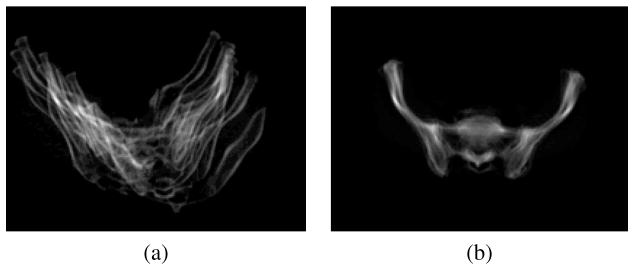
Finally, the subject is registered to the atlas with a 7 degrees of freedom (DOF) similarity transformation (rigid registration + isotropic scaling) using the method by Jenkinson and Smith called FLIRT [17]. This step guarantees that remaining shape variations between the atlas and the patient data are due to the same type of population variations that are represented by the shape statistics in the atlas. This is demonstrated in Fig. 8. The figure shows the average of 10 subjects that have been co-registered using a 7 DOF similarity transform. The 10 images were added both before and after the registration to show how variations due to translation and scale have been removed across the subjects by the similarity transform.

Fig. 8.

Overlay of 10 subjects (a) before registration (b) after registering them to the atlas using 7 DOF similarity registration (rigid + isotropic scaling).

7 Results and Discussion

Mjolnir+ was evaluated on a CT dataset of 51 human male pelvises, 41 of which were used to construct the statistical atlas and 10 that were held out to evaluate the performance of the algorithm. Both visual and quantitative results are presented and compared with results generated by Mjolnir.

7.1 Basic Performance

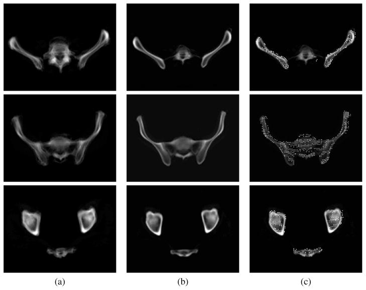
A simple demonstration of the benefits of Mjolnir+ and of its capability to align a tetrahedral mesh is shown in Fig. 9. A total of 10 subject images were registered to the atlas using Mjolnir+ and the average of the 10 registered images computed. The figure shows how the deformable registration compares with the pelvis alignment using 7 DOF similarity registration. The alignment of a tetrahedral mesh to a subject reveals the presence of both surface points and volumetric points residing deep within the bone.

Fig. 9.

Average of 10 subjects (a) after 7 DOF registration (b) after 7 DOF registration followed by deformable registration using shape statistics and topology preservation. (c) The deformable registration result in (b) with the atlas mesh vertices superimposed, revealing the presence of both surface points and volumetric points residing deep within the bone. Three different slices of the 3D images are shown.

7.2 Automatic Segmentation

The pelvises within six (held-out) CT data sets were manually labeled, thereby providing ground truth data for quantitative assessment of registration accuracy. Then, both Mjolnir and Mjolnir+ were used to automatically identify those pelvises through registration. In our evaluation study we measured the quality of overlap using the Dice coefficient defined as [18]

$$D(S_1,S_2)=\frac{2\mid S_1\cap S_2\mid }{(\mid S_1\mid +\mid S_2\mid )},$$ (6)

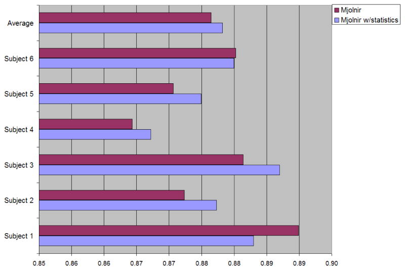
where S₁ and S₂ are the two segmented regions and |S| denotes the number of voxels in S. The Dice coefficient between each of the manually labeled pelvises—i.e., the ground truth—and the automatically determined pelvises were computed; the results are shown in Fig. 10. The average Dice coefficient is slightly higher when using the statistical atlas, however the difference is very subtle and not statistically significant (p-value = 0.4). One reason for the small difference using this measure is that the Dice coefficient was computed over the entire pelvis and the regions showing improvements are small compared to the total number of voxels within the pelvic bone.

Fig. 10.

The Dice coefficient between each of the manually labeled pelvises and the automatically determined pelvises for the two different registration approaches (i.e., with and without prior shape statistics).

In order to investigate this further we constructed triangular surface meshes from the segmented masks and computed the absolute vertex-to-surface error between the automatically labeled pelvises and the manually labeled pelvises. The results are shown in Table I. The mean and standard deviation (SD) of the error were both higher when using Mjolnir (mean: 1.0044 voxels, SD: 0.1085 voxels) than when using Mjolnir+ (mean: 0.9472 voxels, SD: 0.0372 voxels), yielding a more consistent alignment when utilizing the statistical information. Although the difference is not statistically significant (p-value = 0.3) a trend of improvements is evident when looking at Table I. There are two main reasons for these improvements. First, all of the images were acquired with barium in the bowel, which causes extraneous large edges, undesired driving voxel matches, and undesired matches in the absence of statistical information. Second, the subject scans contain femur in the images while the atlas only contains information about the pelvic bone itself. This also causes undesired matches in the absence of statistical information.

Table I.

The absolute vertex-to-surface error (mean ± SD in voxels) between each of the manually labeled pelvises and the automatically determined pelvises for the two different registration approaches (i.e. with and without prior shape statistics).

	Mjolnir	Mjolnir+
Subject 1	0.9957 ± 1.8750	0.9620 ± 1.7659
Subject 2	0.9458 ± 1.4653	0.9052 ± 1.4082
Subject 3	0.9213 ± 1.6762	0.9207 ± 1.7052
Subject 4	1.0401 ± 1.6428	1.0050 ± 1.6557
Subject 5	1.2042 ± 1.8626	0.9243 ± 1.0239
Subject 6	0.9192 ± 0.9853	0.9660 ± 1.1384
Average	1.0044 ± 0.1085	0.9472 ± 0.0372

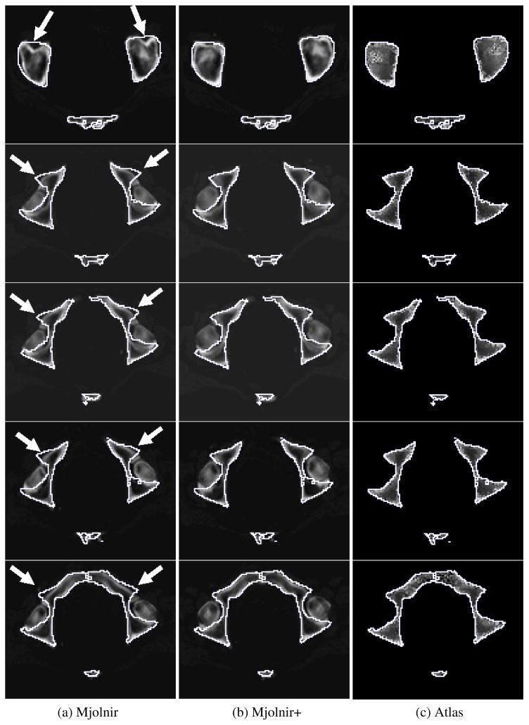
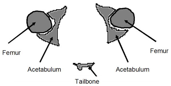
Specific examples of the behavior described above are demonstrated in Figs. 12–15. Fig. 12 demonstrates the challenge of accurately registering the acetabulum (the concave surface of the pelvis where the head of the femur meets the pelvis and forms the hip joint, as shown in Fig. 11) in raw subject scans with atlas data that only contains the pelvic bone and no femur. Large errors are visible around the acetabulum when using Mjolnir [Column (a)] with mesh topology preserved but no statistics. The algorithm tries to “squish” the femur to align with the acetabulum. Mjolnir+ on the other hand, which incorporates prior shape information and topology preservation into Mjolnir, substantially improves the registration/segmentation as shown in Column (b) of the figure. Column (c) shows the atlas image for comparison. The absence of the femur bone should be noted in the atlas image.

Fig. 12.

2D slices from five different subjects are shown. The white contour is the same across each row and represents the outline of the atlas. (a) Deformed subject image revealing large registration/segmentation errors in the acetabulum when using Mjolnir (white arrows) (b) Deformed subject image showing more accurate registration/segmentation when using Mjolnir+. (c) Atlas density image derived from the Bernstein polynomials.

Fig. 15.

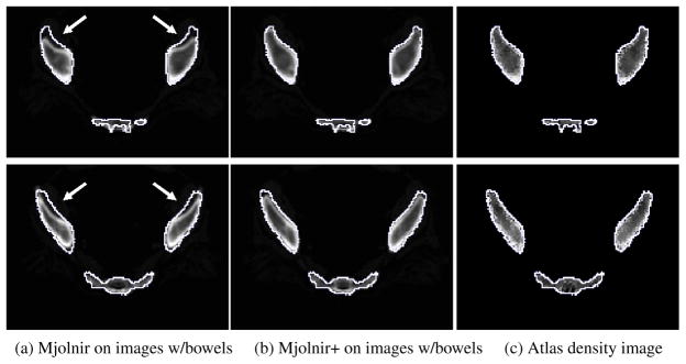
Demonstration of how Mjolnir+ can be used in the challenge of registering scans of subject with barium in the bowel. 2D slices of the 3D image from two different examples are shown. The white contour is the same across each row and represents the outline of the atlas. (a) Registration of raw images (images containing bowels, however, bowels not visible on this slice) using Mjolnir. (b) Registration of raw images using Mjolnir+. (c) Atlas density image derived from the Bernstein polynomials.

Fig. 11.

A cartoon drawing of a cross section through the femur and the acetabular bone of the pelvis.

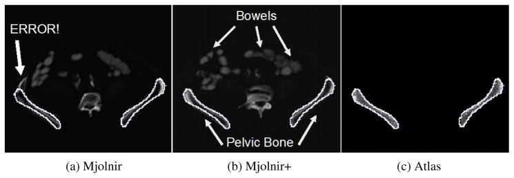
The second challenge when registering raw CT scans with atlas data is when the subject has been administered contrast agents such as barium sulfate. Barium sulfate blocks the passage of x-rays and yields a CT intensity similar to that of bone. This can cause confusion in registration algorithms and limit achievable registration accuracy, as demonstrated in Fig. 13(a). Part of the ilium has been pulled in the direction toward the bowels. With such dramatic differences between the subject scan and the atlas, statistical shape information helps to stabilize the registration, as demonstrated in Fig. 13(b). The artifact caused by the bowels disappears when using Mjolnir+.

Fig. 13.

The challenge of registering scans of subject containing barium in the bowel with atlas data that only contains the pelvic bone. The white contour is the same in all images and represents the outline of the atlas. (a) Registration result using Mjolnir. A part of the ilium bone has been pulled towards the bowel. (b) Registration result using Mjolnir+. (c) Atlas density image derived from the Bernstein polynomials.

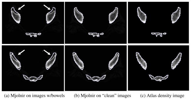
Another example of how barium filled bowels can affect the registration results is demonstrated in Fig. 14. It is not as obvious in these images that the bowels are causing the large errors in the registration results because the bowels are not visible on the slices shown. However, in order to demonstrate the effects of the bowels on the registration we manually removed the bowels from the dataset (a time consuming and tedious procedure) and ran Mjolnir again. The results are shown in Fig. 14(b). The effects of the bowels on the registration have been eliminated by the manual cleaning of the data. Fig. 15 shows how the same negative effects were avoided by using Mjolnir+ [see Column (b)].

Fig. 14.

The effects of barium filled bowels on the registration result can be eliminated by manually removing the bowels from the images. 2D slices of the 3D image from two different examples are shown. The white contour is the same across each row and represents the outline of the atlas. (a) Registration of raw images (images contain bowels, however, bowels not visible on this slice) using Mjolnir. (b) Registration of cleaned images (bowels manually removed) using Mjolnir. (c) Atlas density image derived from the Bernstein polynomials.

7.3 Topology Preservation

We registered 10 pelvis subjects to an atlas CT image using Mjolnir and Mjolnir+. Mjolnir+ automatically generates a deformed mesh, providing mesh instances for each subject, while Mjolnir generates 3D displacement fields but no mesh. For Mjolnir, we used these displacement fields to deform the atlas mesh providing us with deformed mesh instances for each of the 10 subjects. Then we computed the number of flipped tetrahedra in the deformed meshes from both algorithms. The deformed meshes from Mjolnir had on average 5076 flipped tetrahedra (out of a total of 105767 tetrahedra in the mesh) while Mjolnir+ preserved the topology of the mesh for all subjects. Fig. 16(a) shows the location of the flipped tetrahedra highlighted in blue for one of the ten subjects. Fig. 16(b) shows a volume render of a topologically incorrect tetrahedral mesh. Note the holes in the very thin part of the ilium, which could cause problems when, for example, using the mesh to develop statistical models or render Digital Reconstruction Radiographs (DRRs). Finally, Fig. 16(c) shows a volume render of a topologically correct tetrahedral mesh.

Fig. 16.

(a) Flipped tetrahedra highlighted in blue. (b) Volume render of a topologically incorrect tetrahedral mesh. Note the holes in the very thin part of the ilium. (c) Volume render of a topologically correct tetrahedral mesh.

7.4 Runtime

Finally, we ran both Mjolnir and Mjolnir+ on the same computer (Fedora Core 8, eight 3.6GHz Pentium Xeon processors, 15.7GB RAM), processing images of size 256×256×128 voxels. Mjolnir finished in 53 minutes, Mjolnir with topology preservation (but no statistics) finished in 90 minutes, and Mjolnir+ finished in 56 minutes. Mjolnir+ therefore improves robustness and registration accuracy over that of Mjolnir without a significant change in computation time.

8 Discussion

Several methods have been proposed in recent years that use prior shape information to constrain registration. Xue et al. [19] proposed a method that uses Wavelet-PCA to estimate the pdf of high-dimensional displacement fields from a training set to construct effective statistical priors for constraining deformable registration algorithms. Given a dense input displacement field, the field is iteratively projected onto subspaces of valid deformation fields defined by the Wavelet-PCA (referred to as statistical model of deformations (SMD)) and a regularized displacement field is generated according to the priors. The registration method then uses the shape priors to iteratively toggle between HAMMER [11] and the SMD to yield more robust registration. Yao and Taylor [20] proposed a method that uses statistical information to initialize a deformable registration process. The method is divided into three stages: affine transformation, global deformation, and local deformation. The result of each stage is used as an initialization for the next stage. The prior shape information is only used in the global deformation stage, where the statistical mode parameters are optimized to match the atlas with the anatomical structure in the images. Due to the limited number of training models in the statistical atlas, the prior information in the atlas does not include all the variability inherent in the anatomy. To compensate for this, the algorithm completes with a local deformation step to build correspondences between vertices on the atlas and local features in the image and adaptively warp the atlas. As the method uses the prior knowledge only in the second stage to initialize the alignment for the deformable registration stage this method poses the potential that the transformation locks onto incorrect correspondences, caused for instance by the barium filled bowels, as the method drops the statistical information when it enters the deformable registration part. The same thing could occur in the method by Xue et al. because during the registration in HAMMER there is no prior information used to guide the registration.

The major difference between these methods and Mjolnir+ is that Mjolnir+ incorporates the statistical information into the registration process and uses the shape priors along with landmark and feature matching simultaneously to determine the transformation. Mjolnir+ gradually shifts from emphasizing the prior atlas to emphasizing image features; in this way the atlas provides guidance when it is most needed, and does not prevent a final result that accurately matches the data. We note that the method proposed by Wang and Staib [21] also uses prior shape information that is incorporated into a non-rigid registration framework. However, their method was only implemented in 2D and the shape statistics only described boundary points; in contrast, Mjolnir+ is fully 3D and incorporates shape statistics on a dense set of vertices deep within the object.

9 Conclusion

A 3D-3D deformable image registration algorithm that incorporates a statistical atlas comprising a tetrahedral mesh and a point distribution model was presented. The method enforces a valid topology of the deformed mesh and uses the dominant statistical modes of the atlas to guide the deformable registration process. This integration of prior shape information from the statistical modes into the 3D-3D registration provides constant guidance from the atlas throughout the registration process. Experiments showing both visually and quantitatively more robust segmentation with increased registration accuracy were provided, demonstrating the benefits of the new method.

References

- 1.Yao J, Taylor R. Tetrahedral mesh modeling of density data for anatomical atlases and intensity-based registration. Lecture Notes in Computer Science, Proc MICCAI. 2000:531–540. [Google Scholar]
- 2.Davies RhH, Twining CJ, Cootes TF, Waterton JC, Taylor CJ. A minimum description length approach to statistical shape modelling. IEEE Trans Med Imag. 2002;21:525–537. doi: 10.1109/TMI.2002.1009388. [DOI] [PubMed] [Google Scholar]
- 3.Chui H, Rangarajan A, Zhang J, Leonard CM. Unsupervised learning of an atlas from unlabeled point-sets. Pattern Analysis and Machine Intelligence, IEEE Trans on. 2004;26(2):160–172. doi: 10.1109/TPAMI.2004.1262178. [DOI] [PubMed] [Google Scholar]
- 4.Beg MF, Khan A. Computing an average anatomical atlas using LDDMM and geodesic shooting. Proceedings of the IEEE International Symposium on Biomedical Imaging (ISBI) 2006:1116–1119. [Google Scholar]
- 5.Cootes T, Taylor C. Active shape models - smart snakes. Proc Br Machine Vision Conf. 1992:266–275. [Google Scholar]
- 6.Cootes TF, Cooper D, Taylor CJ, Graham J. Active shape models - their training and application. Computer Vision and Image Understanding. 1995;61(1):38–59. [Google Scholar]
- 7.McInerney T, Terzopoulos D. Deformable models in medical image analysis: A survey. Medical Image Analysis. 1996;1(2):91–108156. doi: 10.1016/s1361-8415(96)80007-7. [DOI] [PubMed] [Google Scholar]
- 8.Kaus MR, Pekar V, Lorenz C, Truyen R, Lobregt S, Weese J. Automated 3-D PDM construction from segmented images using deformable models. IEEE Trans Med Imag. 2003;22(8):1005–1013. doi: 10.1109/TMI.2003.815864. [DOI] [PubMed] [Google Scholar]
- 9.Chintalapani Gouthami, Ellingsen Lotta M, Sadowsky Ofri, Prince Jerry L, Taylor Russell H. Statistical atlases of bone anatomy: Construction, iterative improvement and validation. The International Conference on Medical Image Computing and Computer-Assisted Intervention (MICCAI); 2007. [DOI] [PubMed] [Google Scholar]
- 10.Ellingsen LM, Prince JL. Mjolnir: Deformable image registration using feature diffusion. Proceedings of the SPIE Medical Imaging Conference. 2006;6144:329–337. [Google Scholar]
- 11.Shen D, Davatzikos C. HAMMER: Hierarchical attribute matching mechanism for elastic registration. IEEE Trans Med Imag. 2002;21(11):1421–1439. doi: 10.1109/TMI.2002.803111. [DOI] [PubMed] [Google Scholar]
- 12.Mohamed A, Davatzikos C. Finite element mesh generation and remeshing from segmented medical images. Proceedings of the IEEE International Symposium on Biomedical Imaging (ISBI); 2004. pp. 420–423. [Google Scholar]
- 13.Cootes TF, Taylor CJ. Statistical models of appearance for computer vision. 1999 [Google Scholar]
- 14.Ellingsen LM. Ph.D. thesis. Johns Hopkins University; Baltimore, Maryland 21218, USA: 2008. Hybrid Deformable Image Registration – With Application to Brains, Pelvises, and Statistical Atlases. [Google Scholar]
- 15.Prince Jerry L, Links Jonathan M. Medical Imaging Signals and Systems. Pearson Prentice Hall; 2006. [Google Scholar]
- 16.Pham DL. Robust fuzzy segmentation of magnetic resonance images. Proceedings of the Fourteenth IEEE Symposium on Computer-Based Medical Systems (CBMS2001); IEEE Press; 2001. pp. 127–131. [Google Scholar]
- 17.Jenkinson M, Smith SM. A global optimisation method for robust affine registration of brain images. Medical Image Analysis. 2001;5(2):143–156. doi: 10.1016/s1361-8415(01)00036-6. [DOI] [PubMed] [Google Scholar]
- 18.Dice LR. Measures of the amount of ecologic association between species. Ecology. 1945;26:297–302. [Google Scholar]
- 19.Xue Zhong, Shen Dinggang, Davatzikos Christos. Statistical representation of high-dimensional deformation fields with application to statistically-constrained 3D warping. Medical Image Analysis. 2006;10:740–751. doi: 10.1016/j.media.2006.06.007. [DOI] [PubMed] [Google Scholar]
- 20.Yao J, Taylor RH. Non-rigid registration and correspondence in medical image analysis using multiple-layer flexible mesh template matching. International Journal of Pattern Recognition and Artificial Intelligence (IJPRAI) 2003;17(7):1145–1165. [Google Scholar]
- 21.Wang Y, Staib LH. Physical model-based non-rigid registration incorporating statistical shape information. Medical Image Analysis. 2000;4(1):7–21. doi: 10.1016/s1361-8415(00)00004-9. [DOI] [PubMed] [Google Scholar]