Susceptibility Tensor Imaging

Abstract

Heterogeneity of magnetic susceptibility within brain tissues creates unique contrast between gray and white matter in MRI phase images acquired by gradient echo sequences. Detailed understanding of this contrast may provide meaningful diagnostic information. In this communication, we report an observation of extensive anisotropic magnetic susceptibility in the white matter of the central nervous system. Furthermore, we describe a susceptibility tensor imaging (STI) technique to measure and quantify this phenomenon. This technique relies on the measurement of resonance frequency offset at different orientations with respect to the main magnetic field. We propose to characterize this orientation variation using an apparent susceptibility tensor. The susceptibility tensor can be decomposed into three eigenvalues (principal susceptibilities) and associated eigenvectors that are coordinate-system independent. We show that the principal susceptibilities offer strong contrast between gray and white matter while the eigenvectors provide orientation information of an underlying magnetic network. We believe that this network may further offer information of white matter fiber orientation.

Introduction

The Larmor frequency of a nucleus is affected by a number of factors including its intrinsic quantum energy levels determined by nuclear magnetic moment, chemical shifts caused by electronic shielding and magnetic coupling with the surrounding chemical environment. One important form of coupling is conducted through the induced magnetic dipole moment which is proportional to the susceptibility. This induced magnetic moment will oppose the field for diamagnetic materials and be along the field for paramagnetic materials. As a result, magnetic susceptibility results in a resonance frequency shift that can be measured using a gradient-recalled-echo (GRE) sequence.

Traditionally, off-resonant frequency or image phase has been largely discarded due to its poor contrast and the perceived lack of meaningful information except for in a few cases such as phase-contrast imaging where phase is specifically generated to measure flow velocity. In the mid to late 1980s, a number of authors reported the use of susceptibility effect to detect hemorrhage (1-4). In 1987, I.R. Young et al used phase maps to detect changes in the local magnetic field in tumors, lacunar infarct and multiple sclerosis (5). They attributed the effect to the paramagnetic contributions of species such as deoxyhemoglobin, methemoglobin, free ferric iron, hemosiderin, and other breakdown products of blood (5). Later, Haacke at el realized that by multiplying a high-pass filtered phase image with the magnitude image, the contrast between tissue and small vessels can be enhanced dramatically (6,7). The application of susceptibility weighted imaging has grown rapidly in the imaging of veins, microhemmorrhage and neurodegenerative diseases (8,9).

More recently, spurred by the availability of high and ultra-high field strength, contrast existing in the phase image itself has generated a significant amount of interest. Rauscher et al reported that, with background phase removed, phase images showed excellent contrast and revealed anatomic structures that were not visible on the corresponding magnitude images (10,11). Duyn et al recently reported the observation of subtle layered structure in regions between gray and white matter in high-resolution phase images acquired at 7.0 T (12). The specific source of this contrast is still a topic of research. A number of mechanisms have been suggested including iron, proteins and proton exchange (12-17).

Although a phase image provides unique tissue contrast in the brain, such contrast is not the intrinsic property of brain tissue. Phase value depends on a number of factors including time of echo (TE), geometric shape of the brain and spatial distribution of susceptibility. To obtain the intrinsic magnetic susceptibility map, one has to solve a difficult ill-posed inverse problem. A number of recent studies have aimed to improve the accuracy of susceptibility estimation by incorporating regularization techniques (14,18,19). For example, recently Kressler et al used a non-linear regularization method to allow per voxel estimation of magnetic susceptibility (20).

In general, it has been assumed that susceptibility is isotropic (orientation independent) in biologic tissues. Here we report the observation of an orientation dependent magnetic susceptibility in the mouse central nervous system. We propose a method to quantify and make unique images of tissue magnetic anisotropy. This method uses the orientation distribution of magnetic susceptibility to characterize magnetic susceptibility anisotropy (MSA) within biologic tissues. In a second-order approximation, this distribution function is described by an apparent susceptibility tensor (AST). We derive a mathematical relationship between the susceptibility tensor and observed MR signals. The proposed susceptibility-tensor imaging method provides the necessary imaging techniques to acquire and the mathematical tools to quantify susceptibility anisotropy. This anisotropy can be an intrinsic property of tissue or can be purposely induced by the introduction of external molecular agents. As a preliminary demonstration, we have implemented this new imaging technique on an ex vivo mouse brain.

Methods

Apparent Susceptibility Tensor (AST)

In general, magnetic susceptibility can be described by a second-order (or rank 2) tensor χ that is referred to as apparent susceptibility tensor in this paper. Specifically, χ is a 3×3 matrix whose elements are denoted as χ_ij. For isotropic susceptibility, this tensor will be diagonal with equal diagonal elements. Given a spatial distribution of susceptibility tensors, the magnetic flux density vector B seen by each nucleus is related to the macroscopic flux density B₀ as (21,22)

$$\mathbf{B}=(\mathbf{I}-\mathrm{\sigma }\mathbf{I}-\frac{2}{3}\mathbf{\chi }){\mathbf{B}}_{\mathbf{0}}$$ [1]

Here, I is the identity matrix; σ is the chemical shift caused by electronic screening effect. Notice that vacuum permeability μ₀ is assumed to be one for simplicity. The macroscopic flux density B₀ is further related to the applied magnetic field vector H and the demagnetizing field h following

$${\mathbf{B}}_{\mathbf{0}}=(\mathbf{I}+\mathbf{\chi })\mathbf{H}(+\mathbf{h})$$ [2]

The demagnetizing field is necessary in order to satisfy Maxwell’s equations and is introduced by the loading of an object into a magnetic field. For modern superconductor MRI scanners, we can assume h ≪H. For biological samples that are MRI compatible, it can also be assumed that their magnetic susceptibility is small so that χ_ij ≪1. Substituting Eq. [2] into Eq. [1] and keeping only the first-order terms, we obtain

$$\mathbf{B}=(\mathbf{I}-\mathrm{\sigma }\mathbf{I}+\frac{1}{3}\mathbf{\chi })\mathbf{H}(+\mathbf{h})$$ [3]

The demagnetizing field can be obtained by subjecting Eq. [3] to Maxwell’s equations. Specifically, the divergence of the flux density is zero, that is

$$\nabla \mathbf{·}\mathbf{B}=0$$ [4]

Furthermore, Eq. [4] is also valid in the absence of loading. In other words, when only the applied external field is present, we obtain

$$\nabla \mathbf{·}\mathbf{H}=0$$ [5]

Combining Eqs. [3], [4] and [5] while keeping terms up to the first order, we obtain

$$\mathbf{H}\mathbf{·}(\nabla \mathbf{·}\mathrm{\chi })+\nabla \mathbf{·}\mathbf{h}=0$$ [6]

Solving Eq. [6] results in the following formula for the demagnetizing field

$$\mathbf{h}=-{\mathit{FT}}^{-1}\left\{\mathbf{k}\frac{{\mathbf{k}}^{\mathbf{T}}\mathit{FT}\left\{\mathbf{\chi }\right\}\mathbf{H}}{k^2}\right\}$$ [7]

Here, the superscript T represents the transpose operation. Finally, by substituting Eq. [7] into Eq. [3] and keeping terms up to the first-order, we found that the off-resonance field ΔB, referenced to (1-σ)H, can be expressed as

$$\mathbf{\Delta }\mathbf{B}={\mathit{FT}}^{-1}\left\{\frac{1}{3}\mathit{FT}\left\{\mathbf{\chi }\right\}\mathbf{H}-\mathbf{k}\frac{{\mathbf{k}}^{\mathbf{T}}\mathit{FT}\left\{\mathbf{\chi }\right\}\mathbf{H}}{k^2}\right\}$$ [8]

In MRI, what we can observe is image phase or frequency offset rather than the full vector ΔB. The observable phase in the subject frame of reference can be expressed as

$$\theta ={\mathit{FT}}^{-1}\left\{\frac{1}{3}{\widehat{\mathbf{H}}}^{\mathbf{T}}\mathit{FT}\left\{\mathbf{\chi }\right\}\widehat{\mathbf{H}}-\widehat{\mathbf{H}}\mathbf{·}\mathbf{k}\frac{{\mathbf{k}}^{\mathbf{T}}\mathit{FT}\left\{\mathbf{\chi }\right\}\widehat{\mathbf{H}}}{k^2}\right\}\gamma \mathit{Ht}$$ [9]

In the laboratory frame of reference, it is expressed as

$$\theta ={\mathit{FT}}^{-1}\left\{\frac{1}{3}\mathit{FT}\left\{{\chi }_{33}\right\}-\frac{k_3^2}{k^2}\mathit{FT}\left\{{\chi }_{33}\right\}\right\}\gamma \mathit{Ht}$$ [10]

Here, H is the magnitude of the applied magnetic field; Ĥ is the unit vector of the applied magnetic field; t is the TE in a gradient echo sequence. If a sufficient number of independent measurements are available, Eq. [9] and Eq. [10] can be inverted to determine χ. In principle, the h choice of the frame of reference should not affect the accuracy of the calculated magnetic susceptibility tensor. When the subject frame of reference is used, the susceptibility tensor in Eq. [9] remains the same for each orientation; only the magnetic field vector is rotated accordingly. When the laboratory frame of reference is used, the susceptibility tensor in Eq. [10] is rotated according to RχR^T while the magnetic field vector remains along the z-axis. Here R is the rotation matrix from the subject frame of reference to the laboratory frame of reference.

Determination of AST

Assuming that the susceptibility tensor is symmetric, then there are six independent variables to be determined for each tensor. In principle, a minimum of six independent measurements are necessary and they can be acquired at different relative orientations between the subject and main magnetic field. A set of independent measurements can be obtained by rotating the imaging object with respect to the main magnetic field. Given a set of such measurements, a susceptibility tensor can be estimated by inverting the system of linear equations formed by Eq. [9] in the subject frame of reference or by Eq. [10] in the laboratory frame of reference. The steps involved in both frames of reference are outlined in Figure 1.

Figure 1.

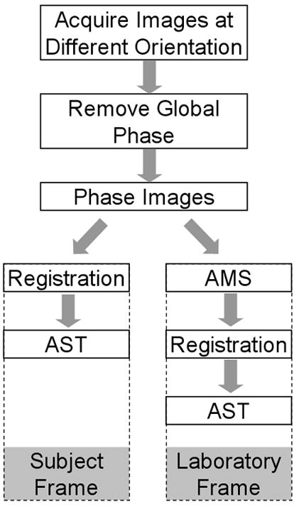
Algorithmic flow chart for measuring apparent susceptibility tensor. Susceptibility tensor can be measured either in the subject frame of reference or in the laboratory frame of reference. In the subject frame, the apparent susceptibility tensor is computed directly from registered phase images. In the laboratory frame, an apparent magnetic susceptibility (AMS) is first computed for each orientation and then used to compute the AST.

As an illustration, we will demonstrate the solution in the subject frame of reference. In this frame of reference, images acquired at different orientations need to be first co-registered to a chosen reference orientation. The six rigid-body transformation parameters are first estimated using magnitude images. The estimated transformation matrix is then used to register and re-slice the real and imaginary part separately. Phase maps are computed from the registered real and imaginary parts. A smooth global phase is subtracted from the phase maps. Once all phase maps are computed, an apparent susceptibility tensor is computed voxel-by-voxel. Specifically, by taking a Fourier transform of both sides of Eq. [9], we can rewrite the equation as

$$\mathit{FT}\left\{\stackrel{\sim }{\theta }\right\}=(\frac{1}{3}{\widehat{\mathbf{H}}}^{\mathbf{T}}\mathit{FT}\left\{\mathbf{\chi }\right\}\widehat{\mathbf{H}}-\mathbf{k}\mathbf{·}\widehat{\mathbf{H}}\frac{{\mathbf{k}}^{\mathbf{T}}\mathit{FT}\left\{\mathbf{\chi }\right\}\widehat{\mathbf{H}}}{k^2})$$ [11]

Here, θ̃ is the normalized phase

$$\stackrel{\sim }{\theta }=\frac{\theta }{\gamma \mathit{Ht}}$$ [12]

Given a set of n measurements, we can define, in the frequency domain, a measurement vector θ̃, a vector of unknowns x and a system matrix A as follows

$$\stackrel{\sim }{\mathbf{\theta }}={\left[{\stackrel{\sim }{\theta }}_1(\mathbf{k}){\stackrel{\sim }{\theta }}_2(\mathbf{k})\dots {\stackrel{\sim }{\theta }}_n(\mathbf{k})\right]}^{\mathbf{T}}$$ [13]

$$\mathbf{x}={\left[{\chi }_{11}(\mathbf{k}){\chi }_{12}(\mathbf{k}){\chi }_{13}(\mathbf{k}){\chi }_{22}(\mathbf{k}){\chi }_{33}(\mathbf{k})\right]}^{\mathbf{T}}$$ [14]

$$\mathbf{A}=\left[\begin{array}{cccc}\frac{1}{3}{\stackrel{⌢}{H}}_1^{(1)}{\stackrel{⌢}{H}}_1^{(1)}-\mathbf{k}\mathbf{·}{\stackrel{⌢}{\mathbf{H}}}^{(1)}\frac{k_1{\stackrel{⌢}{H}}_1^{(1)}}{k^2}& \frac{2}{3}{\stackrel{⌢}{H}}_1^{(1)}{\stackrel{⌢}{H}}_2^{(1)}-\mathbf{k}\mathbf{·}{\stackrel{⌢}{\mathbf{H}}}^{(1)}\frac{k_1{\stackrel{⌢}{H}}_2^{(1)}+k_2{\stackrel{⌢}{H}}_1^{(1)}}{k^2}& \cdots & \frac{1}{3}{\stackrel{⌢}{H}}_3^{(1)}{\stackrel{⌢}{H}}_3^{(1)}-\mathbf{k}\mathbf{·}{\stackrel{⌢}{H}}^{(1)}\frac{k_3{\stackrel{⌢}{H}}_3^{(1)}}{k^2}\\ \frac{1}{3}{\stackrel{⌢}{H}}_1^{(2)}{\stackrel{⌢}{H}}_1^{(2)}-\mathbf{k}\mathbf{·}{\stackrel{⌢}{\mathbf{H}}}^{(2)}\frac{k_1{\stackrel{⌢}{H}}_1^{(2)}}{k^2}& \frac{2}{3}{\stackrel{⌢}{H}}_1^{(2)}{\stackrel{⌢}{H}}_2^{(2)}-\mathbf{k}\mathbf{·}{\stackrel{⌢}{\mathbf{H}}}^{(2)}\frac{k_1{\stackrel{⌢}{H}}_2^{(2)}+k_2{\stackrel{⌢}{H}}_1^{(2)}}{k^2}& \cdots & \frac{1}{3}{\stackrel{⌢}{H}}_3^{(2)}{\stackrel{⌢}{H}}_3^{(2)}-\mathbf{k}\mathbf{·}{\stackrel{⌢}{\mathbf{H}}}^{(2)}\frac{k_3{\stackrel{⌢}{H}}_3^{(2)}}{k^2}\\ ⋮& ⋮& ⋮& ⋮\\ \frac{1}{3}{\stackrel{⌢}{H}}_1^{(n)}{\stackrel{⌢}{H}}_1^{(n)}-\mathbf{k}\mathbf{·}{\stackrel{⌢}{\mathbf{H}}}^{(n)}\frac{k_1{\stackrel{⌢}{H}}_1^{(n)}}{k^2}& \frac{2}{3}{\stackrel{⌢}{H}}_1^{(n)}{\stackrel{⌢}{H}}_2^{(n)}-\mathbf{k}\mathbf{·}{\stackrel{⌢}{\mathbf{H}}}^{(n)}\frac{k_1{\stackrel{⌢}{H}}_2^{(n)}+k_2{\stackrel{⌢}{H}}_1^{(n)}}{k^2}& \cdots & \frac{1}{3}{\stackrel{⌢}{H}}_3^{(n)}{\stackrel{⌢}{H}}_3^{(n)}-\mathbf{k}\mathbf{·}{\stackrel{⌢}{\mathbf{H}}}^{(n)}\frac{k_3{\stackrel{⌢}{H}}_3^{(n)}}{k^2}\end{array}\right]$$ [15]

The resultant system of linear equations can be solved voxe-by-voxel using least-squares estimation as

$$\mathbf{x}={({\mathbf{A}}^{\mathbf{T}}\mathbf{A})}^{-1}{\mathbf{A}}^{\mathbf{T}}\stackrel{\sim }{\mathbf{\theta }}$$ [16]

Once x is computed for each voxel, the entries of the susceptibility tensor can be obtained through a 3D inverse Fourier transform.

The inverse problem of computing a susceptibility map based on a phase image is a well-known ill-posed problem due to the existence of zero coefficients in the right-hand side of Eq. [11]. This difficulty can be alleviated through numerical regularization (18-20,23) or by acquiring a set of phase images at different orientations with respect to the main field (24). In our case, the matrix defined in Eq. [15] is generally well conditioned because of the availability of multiple independent measurements. To further improve the accuracy of the estimation, we applied the algorithm of least squares using orthogonal and right triangular decomposition (LSQR) (25) that has been widely used for solving ill-conditioned linear system of equations. In this study, we used the implementation of LSQR by Matlab (Version 7, Release 14, The MathWorks Inc.) with the default stopping criteria.

The computed tensor is coordinate system dependent. To define rotational invariant quantities, we perform eigenvalue decomposition of the measured tensor and define three principal susceptibilities. We denote the three principal susceptibilities as χ₁, χ₂, and χ₃ , ranked in a descending order, each with a corresponding eigenvector. The major eigenvector points toward the direction that exhibits the largest magnetic susceptibility. Using the major eigenvector, we further define a color-coding scheme for the major principal susceptibility χ₁ as follows: red represents anterior-posterior direction, green represents left-right and blue represents superior-inferior.

Experimental setup

As a demonstration, we have conducted an STI experiment on an ex vivo mouse brain on a small-bore 7T MRI scanner equipped with a shielded coil providing gradients of 160 G/cm. The animal study was approved by the Institutional Animal Care and Use Committee (IACUC) Duke University. Adult (9–12 weeks) C57BL/6 mice [The Jackson Laboratory, Bar Harbor, ME; Charles River, Raleigh, NC]) were anesthetized and perfused following Jonson et al (26,27). The perfused mouse brain was kept within the skull to prevent any potential damage to the brain caused by surgical removal. The specimen was sealed tightly inside a cylindrical tube (length 30mm and diameter 11mm). To allow free rotation, the tube was contained within and taped to a hollow sphere (diameter ~30mm). The sphere containing the specimen was placed inside a dual-channel mouse coil (diameter ~30mm, M2M imaging Corp, Cleveland OH). Ultra-high resolution 3D SPGR images were acquired using the imaging parameters: matrix size = 256×256×256, field-of-view (FOV) = 22×22×22 mm³, flip angle = 60°, TE = 8 ms, and TR = 100 ms. After each acquisition, the sphere was rotated to a different orientation and the acquisition was repeated. The FOV was chosen to be larger than the specimen and was kept the same throughout the scan such that, when the specimen was rotated, it remained within the FOV. A total of 19 orientations were sampled which roughly cover the spherical surface evenly. To avoid shimming introduced frequency shift, the same shimming currents were applied for all directions. The carrier frequency was also kept the same. MR signals were demodulated at this frequency, thus, the measured frequency shift and susceptibility map is also referenced to this frequency. Temperature was monitored throughout the scans and fluctuation was recorded to be below 1°C.

Results

A 3D frequency map was calculated for each orientation. Examples of these maps are shown in Figure 2. Although the frequency maps clearly indicate an orientation dependency, this variation is a result of both a spatially distributed susceptibility and a geometric factor. Thus it is not a definitive evidence of bulk susceptibility anisotropy.

Figure 2.

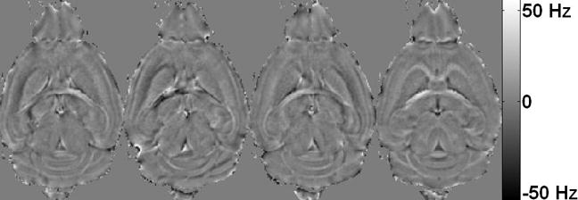
Maps of frequency shift measured at four different orientations out of a total of 19 orientations. The resonance frequency of protons within white matter varies dramatically from one orientation to another. On the contrary, the resonance frequency is relatively consistent within the gray matter. As a result, the contrast between gray and white matter appears vastly different at different orientations.

An apparent susceptibility tensor was computed for each voxel. Figure 3 shows three representative elements of the measured susceptibility tensor from three representative slices. The anisotropy existing in the tensor is clearly evident from the varying contrast between different tensor elements. The anisotropy appears the strongest in white matter while it remains relatively weak in the gray matter. We emphasize that the observed anisotropy is not a consequence of the tensor model. Even isotropic medium can be described by a diagonal tensor with equal diagonal entries.

Figure 3.

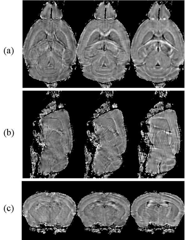
Three elements of AST from three representative slices. (a) Tensor element χ₁₁, χ₂₃ and χ₃₃ from a dorsal slice. (b) The same three elements from a sagittal slice and (d) from a coronal slice. The existence of off diagonal entries and the difference between diagonal entries are clear evidence of magnetic susceptibility anisotropy.

The measured susceptibility tensor is further decomposed into three eigenvectors and three associated eigenvalues denoted as χ₁, χ₂, and χ₃ in a descending order. Examples of eigenvalue maps and the corresponding mean susceptibility maps are shown in Figure 4. The maximal principal susceptibility χ₁ demonstrates the strongest contrast between gray and white matter. In fact, χ₁ provides a contrast that is strikingly similar to a fractional anisotropy map computed by diffusion tensor imaging. The maximal principal susceptibility is further color-coded based on the direction of the associated eigenvector. The color-coding scheme is as follows: red representing anterior-posterior direction, green representing left-right, and blue representing dorsal-ventral. The color-coded principal susceptibility is shown in Figure 5.

Figure 4.

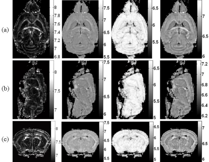
Principal susceptibility and mean susceptibility maps (10^-8 SI units). (a) Shown from left to right are the maximal principal susceptibility χ₁ , the median principal susceptibility χ₂ , the minimal principal susceptibility χ₃ and the mean susceptibility respectively of a dorsal slice, (b) of a sagittal slice and (c) of a coronal slice. The maximal principal susceptibility offers the strongest contrast between gray and white matter that is similar to diffusion fractional anisotropy.

Figure 5.

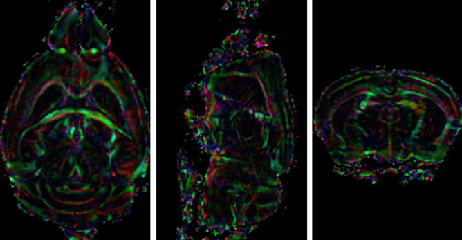
Color-coded maximal principal susceptibility maps from three representative slices. The color is defined by the eigenvector associated with the maximal principal susceptibility with red representing anterior-posterior direction, green representing left-right, and blue representing dorsal-ventral. The color intensity is scaled by the maximal principal susceptibility value.

Discussions

Our results reveal extensive susceptibility anisotropy within the central nervous system that has not been demonstrated before. We have also shown that this anisotropy can be measured by MRI. Mathematically, susceptibility anisotropy can be effectively described by a second order tensor. One advantage of the tensor description is that coordinate independent quantities can be defined through eigenvalue decomposition. The resulting principal susceptibility maps not only provide a quantitative measure of magnetic susceptibility anisotropy but also offer a unique image contrast.

Brain tissues contain various amounts of iron and iron-carrying macromolecules. These iron and macromolecules possess an intrinsic magnetic susceptibility tensor that is determined by the property of the iron, the structural configuration of the macromolecules and the dipolar coupling between different nuclei. Once these irons and macromolecules are bonded with local tissue structure, additional constraints are imposed on the orientation of the macromolecules thus affecting the apparent susceptibility tensor observed within one voxel. Because of tissue heterogeneity, tensor values will be different for different tissues, thus providing a unique mechanism to enhance tissue contrast. This contrast can be displayed as tensor elements, eigenvalues and eigenvectors, or a combination of them such as a magnitude image weighted by eigenvalues. Tissue structural changes caused by tumor, stroke, traumatic injury and iron-content changes caused by developmental iron deficiency and aging will then manifest in the changes of those quantities.

One clear obstacle in quantifying susceptibility anisotropy in vivo using the proposed technique is the requirement to acquire phase images at different subject orientations with respect to the main magnetic field. In principle, different orientations can be achieved by either rotating the main field or rotating the subject. The design of modern MRI scanners, unfortunately, prohibits the rotation of main field. Rotating a subject within receiving coils is obviously inconvenient and impractical in most scenarios. For the specific case of in vivo brain imaging, rotation about the left-right axis is restricted to approximately within 60° in a supine position; rotation about the anterior-posterior axis is approximately limited within 60 °; rotation about the superior-inferior axis is slightly more flexible at a range of approximately 120°. Besides the logistic difficulty of rotating the head inside the scanner bore, the limited range of rotation angles also poses an additional numerical challenge in solving Eq. [11] due to the worsening of the matrix condition. The potential of STI for small animal imaging, however, is clear as demonstrated in our data. The improved contrast provides yet one more tool for characterizing the structure in genetic models, in disease models, and in a wide range of basic sciences. At the same time, studies in these same models will help elucidate the underlying mechanism and provide the basic underpinnings to permit translation of the technique from mouse to man.

Susceptibility anisotropy is not only an intrinsic property of brain tissue; it can also be potentially induced by the introduction of exogenous agents. It is conceivable that a specific molecular contrast agent can be designed to enhance local tissue susceptibility anisotropy that can be detected by the proposed susceptibility tensor imaging. For example, these contrast molecules can be designed to allow certain preferable binding configuration with tissue macromolecules. Imaging of this class of molecular contrast agent will not simply rely on a T1 or T2* effect. Rather, it will rely on the anisotropic magnetic field generated by these agents.

An important potential application of STI is for mapping 3D white matter fiber pathways in the CNS. Our results strongly suggest that there is a correlation between apparent susceptibility tensor and fiber orientation. The exact relationship is currently under investigation. Currently, diffusion tensor imaging is the only noninvasive method for visualizing whole brain white matter fiber tracts (28-33). There has been a long standing need for alternative methods that can potentially cross validate DTI results. The spatial resolution of DTI has also been very poor compared to structural imaging. In addition, DTI has encountered significant obstacles at ultra-high field strength due to enhanced field inhomogeneity, shortened T2/T2* relaxation time and increased tissue heating. It is still unclear whether high-resolution whole-brain DTI will be practical at ultra-high field strength. STI, on the other hand, relies on low flip angle GRE sequences and benefits from enhanced susceptibility contrast, thus it is ideally suited for ultra-high field imaging.

Conclusions

In conclusion, we demonstrated the existence of extensive magnetic susceptibility anisotropy in the central nervous system. We described a method to measure and quantify this observed anisotropy with an apparent susceptibility tensor. The proposed susceptibility tensor imaging technique opens up new avenues for image contrast generation by using either intrinsic tissue property or external molecular agents. Furthermore, STI provides a framework for a potential alternative fiber tracking method that differs fundamentally from diffusion-based tractography method. However, due to the necessity of rotating the subject in the magnet, the primary application of STI currently will be in small-animal and specimen imaging.

References

- 1.Edelman RR, Johnson K, Buxton R, Shoukimas G, Rosen BR, Davis KR, Brady TJ. MR of hemorrhage: a new approach. AJNR Am J Neuroradiol. 1986;7(5):751–756. [PMC free article] [PubMed] [Google Scholar]
- 2.Gomori JM, Grossman RI, Goldberg HI, Zimmerman RA, Bilaniuk LT. Intracranial hematomas: imaging by high-field MR. Radiology. 1985;157(1):87–93. doi: 10.1148/radiology.157.1.4034983. [DOI] [PubMed] [Google Scholar]
- 3.Winkler ML, Olsen WL, Mills TC, Kaufman L. Hemorrhagic and nonhemorrhagic brain lesions: evaluation with 0.35-T fast MR imaging. Radiology. 1987;165(1):203–207. doi: 10.1148/radiology.165.1.3628772. [DOI] [PubMed] [Google Scholar]
- 4.Winkler M, Higgins CB. Suspected intracardiac masses: evaluation with MR imaging. Radiology. 1987;165(1):117–122. doi: 10.1148/radiology.165.1.3628757. [DOI] [PubMed] [Google Scholar]
- 5.Young IR, Khenia S, Thomas DG, Davis CH, Gadian DG, Cox IJ, Ross BD, Bydder GM. Clinical magnetic susceptibility mapping of the brain. J Comput Assist Tomogr. 1987;11(1):2–6. doi: 10.1097/00004728-198701000-00002. [DOI] [PubMed] [Google Scholar]
- 6.Haacke EM, Xu Y, Cheng YC, Reichenbach JR. Susceptibility weighted imaging (SWI) Magn Reson Med. 2004;52(3):612–618. doi: 10.1002/mrm.20198. [DOI] [PubMed] [Google Scholar]
- 7.Haddar D, Haacke E, Sehgal V, Delproposto Z, Salamon G, Seror O, Sellier N. Susceptibility weighted imaging. Theory and applications. J Radiol. 2004;85(11):1901–1908. doi: 10.1016/s0221-0363(04)97759-1. [DOI] [PubMed] [Google Scholar]
- 8.Haacke EM, DelProposto ZS, Chaturvedi S, Sehgal V, Tenzer M, Neelavalli J, Kido D. Imaging cerebral amyloid angiopathy with susceptibility-weighted imaging. AJNR Am J Neuroradiol. 2007;28(2):316–317. [PMC free article] [PubMed] [Google Scholar]
- 9.Haacke EM, Mittal S, Wu Z, Neelavalli J, Cheng YC. Susceptibility-weighted imaging: technical aspects and clinical applications, part 1. AJNR Am J Neuroradiol. 2009;30(1):19–30. doi: 10.3174/ajnr.A1400. [DOI] [PMC free article] [PubMed] [Google Scholar]
- 10.Rauscher A, Barth M, Reichenbach JR, Stollberger R, Moser E. Automated unwrapping of MR phase images applied to BOLD MR-venography at 3 Tesla. J Magn Reson Imaging. 2003;18(2):175–180. doi: 10.1002/jmri.10346. [DOI] [PubMed] [Google Scholar]
- 11.Rauscher A, Sedlacik J, Barth M, Mentzel HJ, Reichenbach JR. Magnetic susceptibility-weighted MR phase imaging of the human brain. AJNR Am J Neuroradiol. 2005;26(4):736–742. [PMC free article] [PubMed] [Google Scholar]
- 12.Duyn JH, van Gelderen P, Li TQ, de Zwart JA, Koretsky AP, Fukunaga M. High-field MRI of brain cortical substructure based on signal phase. Proc Natl Acad Sci U S A. 2007;104(28):11796–11801. doi: 10.1073/pnas.0610821104. [DOI] [PMC free article] [PubMed] [Google Scholar]
- 13.Shmueli K, Li T-Q, Yao B, Fukunaga M, Duyn JH. The contribution of exchange to MRI phase contrast in the human brain. Neuroimage. 2009;47(1):S72. [Google Scholar]
- 14.Haacke EM, Ayaz M, Khan A, Manova ES, Krishnamurthy B, Gollapalli L, Ciulla C, Kim I, Petersen F, Kirsch W. Establishing a baseline phase behavior in magnetic resonance imaging to determine normal vs abnormal iron content in the brain. J Magn Reson Imaging. 2007;26(2):256–264. doi: 10.1002/jmri.22987. [DOI] [PubMed] [Google Scholar]
- 15.Lee J, Hirano Y, Fukunaga M, Silva AC, Duyn JH. On the contribution of deoxy-hemoglobin to MRI gray-white matter phase contrast at high field. Neuroimage. 2009;49(1):193–198. doi: 10.1016/j.neuroimage.2009.07.017. [DOI] [PMC free article] [PubMed] [Google Scholar]
- 16.Yao B, Li TQ, Gelderen P, Shmueli K, de Zwart JA, Duyn JH. Susceptibility contrast in high field MRI of human brain as a function of tissue iron content. Neuroimage. 2009;44(4):1259–1266. doi: 10.1016/j.neuroimage.2008.10.029. [DOI] [PMC free article] [PubMed] [Google Scholar]
- 17.Zhong K, Leupold J, von Elverfeldt D, Speck O. The molecular basis for gray and white matter contrast in phase imaging. Neuroimage. 2008;40(4):1561–1566. doi: 10.1016/j.neuroimage.2008.01.061. [DOI] [PubMed] [Google Scholar]
- 18.Li L, Leigh JS. Quantifying arbitrary magnetic susceptibility distributions with MR. Magn Reson Med. 2004;51(5):1077–1082. doi: 10.1002/mrm.20054. [DOI] [PubMed] [Google Scholar]
- 19.de Rochefort L, Brown R, Prince MR, Wang Y. Quantitative MR susceptibility mapping using piece-wise constant regularized inversion of the magnetic field. Magn Reson Med. 2008;60(4):1003–1009. doi: 10.1002/mrm.21710. [DOI] [PubMed] [Google Scholar]
- 20.Kressler B, de Rochefort L, Liu T, Spincemaille P, Jiang Q, Wang Y. Nonlinear Regularization for Per Voxel Estimation of Magnetic Susceptibility Distributions From MRI Field Maps. IEEE Trans Med Imaging. 2010;29(2):273–281. doi: 10.1109/TMI.2009.2023787. [DOI] [PMC free article] [PubMed] [Google Scholar]
- 21.Li L. Magnetic susceptibility quantification for arbitrarily shaped objects in inhomogeneous fields. Magn Reson Med. 2001;46(5):907–916. doi: 10.1002/mrm.1276. [DOI] [PubMed] [Google Scholar]
- 22.Salomir R, DSB, Moonen CTW. A fast calculation method for magnetic field inhomogeneity due to an arbitrary distribution of bulk susceptibility. Concepts in Magnetic Resonance Part B. 2003;19B(1):26–34. [Google Scholar]
- 23.Kressler B, de Rochefort L, Liu T, Spincemaille P, Jiang Q, Wang Y. Nonlinear Regularization for Per Voxel Estimation of Magnetic Susceptibility Distributions From MRI Field Maps. IEEE Trans Med Imaging. 2009 doi: 10.1109/TMI.2009.2023787. [DOI] [PMC free article] [PubMed] [Google Scholar]
- 24.Liu T, Spincemaille P, de Rochefort L, Kressler B, Wang Y. Calculation of susceptibility through multiple orientation sampling (COSMOS): a method for conditioning the inverse problem from measured magnetic field map to susceptibility source image in MRI. Magn Reson Med. 2009;61(1):196–204. doi: 10.1002/mrm.21828. [DOI] [PubMed] [Google Scholar]
- 25.Saunders M. Solution of sparse rectangular systems using LSQR and CRAIG. BIT Numerical Mathematics. 1995;35(4):588–604. [Google Scholar]
- 26.Johnson GA, Ali-Sharief A, Badea A, Brandenburg J, Cofer G, Fubara B, Gewalt S, Hedlund LW, Upchurch L. High-throughput morphologic phenotyping of the mouse brain with magnetic resonance histology. Neuroimage. 2007;37(1):82–89. doi: 10.1016/j.neuroimage.2007.05.013. [DOI] [PMC free article] [PubMed] [Google Scholar]
- 27.Johnson GA, Cofer GP, Fubara B, Gewalt SL, Hedlund LW, Maronpot RR. Magnetic resonance histology for morphologic phenotyping. J Magn Reson Imaging. 2002;16(4):423–429. doi: 10.1002/jmri.10175. [DOI] [PubMed] [Google Scholar]
- 28.Basser PJ. Inferring microstructural features and the physiological state of tissues from diffusion-weighted images. NMR Biomed. 1995;8(7-8):333–344. doi: 10.1002/nbm.1940080707. [DOI] [PubMed] [Google Scholar]
- 29.Basser PJ, Mattiello J, LeBihan D. Estimation of the effective self-diffusion tensor from the NMR spin echo. J Magn Reson B. 1994;103(3):247–254. doi: 10.1006/jmrb.1994.1037. [DOI] [PubMed] [Google Scholar]
- 30.Basser PJ, Pajevic S, Pierpaoli C, Duda J, Aldroubi A. In vivo fiber tractography using DT-MRI data. Magn Reson Med. 2000;44(4):625–632. doi: 10.1002/1522-2594(200010)44:4<625::aid-mrm17>3.0.co;2-o. [DOI] [PubMed] [Google Scholar]
- 31.Conturo TE, Lori NF, Cull TS, Akbudak E, Snyder AZ, Shimony JS, McKinstry RC, Burton H, Raichle ME. Tracking neuronal fiber pathways in the living human brain. Proc Natl Acad Sci U S A. 1999;96(18):10422–10427. doi: 10.1073/pnas.96.18.10422. [DOI] [PMC free article] [PubMed] [Google Scholar]
- 32.Mori S, Crain BJ, Chacko VP, van Zijl PC. Three-dimensional tracking of axonal projections in the brain by magnetic resonance imaging. Ann Neurol. 1999;45(2):265–269. doi: 10.1002/1531-8249(199902)45:2<265::aid-ana21>3.0.co;2-3. [DOI] [PubMed] [Google Scholar]
- 33.Liu C, Bammer R, Acar B, Moseley ME. Characterizing non-Gaussian diffusion by using generalized diffusion tensors. Magn Reson Med. 2004;51(5):924–937. doi: 10.1002/mrm.20071. [DOI] [PubMed] [Google Scholar]