Accuracy and cut-off point selection in three-class classification problems using a generalization of the Youden index

Summary

We study properties of the index J₃, defined as the accuracy, or the maximum correct classification, for a given three-class classification problem. Specifically, using J₃ one can assess the discrimination between the three distributions and obtain an optimal pair of cut-off points c₁ < c₂ in the sense that the sum of the correct classification proportions will be maximized. It also serves as the generalization of the Youden index in three-class problems. Parametric and non-parametric approaches for estimation and testing are considered and methods are applied to data from an MRS study on HIV patients.

1 Introduction

A number of questions have to be answered before the wide-scale use of a marker. For example, the marker n-acetyl-aspartate over creatine (NAA/Cr) measured by Magnetic Resonance Spectroscopy (MRS) has been widely considered as a marker of neuronal metabolism in the brain [1]. Consequently, it has been suggested that NAA/Cr may be decreased in the brain of HIV-infected subjects with neurological disease secondary to their HIV disease [2]. Thus, when the outcome is binary such as, for example, neurologically impaired (diseased) versus non-impaired (non-diseased), the first step in the validation of the marker is to assess whether the marker significantly discriminates the diseased and non-diseased populations based on the distributions of the marker measurements in the two classes. Specifically, a cut-off point in the marker levels is considered and subjects with marker levels below (above) the cut-off point are identified as “diseased”, while those with marker levels above (below) the cut-off point are considered as “non-diseased”. Receiver Operating Characteristic (ROC) curve analysis is the most widespread technique used in marker validation when there are two disease classes. The ROC curve is the plot, on the unit square, of the true positive rate (the proportion of times the marker identifies a diseased individual as such) versus the false positive rate (the proportion of times the marker erroneously identifies a non-diseased individual as diseased) at each cut-off point. Better markers have higher true positive rates (sensitivity) than false positive rates at each cutoff point, resulting in an ROC curve that lies above the diagonal between the origin and the point (1,1). The index of the area under the ROC curve (AUC) reflects the amount of discrimination of the marker-level distributions in the two samples of subjects derived from the non-diseased and diseased populations, X₁,…,X_n sampled from distribution F and Y₁,…, Y_m sampled from distribution G, respectively. The empirical AUC estimates the probability P(X < Y), which quantifies the discrimination of F and G. Formal assessment of the statistical significance of the AUC index is described comprehensively in [3].

After a marker has been shown to discriminate between diseased and non-diseased populations, the next step involves the selection of an optimal cut-off point based on which a diagnosis will be made. Approaches for the selection of the optimal cut-off point in the framework of ROC analysis are discussed in [3]-[5]. Another approach for the assessment of the discrimination of the diseased and non-diseased populations and cut-off point selection involves the use of a maximally selected statistic chosen to maximize a measure of difference between the two groups. Maximally selected statistics for the two-class case have been studied in [6]- [10] among others. Gail and Green [11] considered a generalization of the Youden index as the selected statistic of interest and made the important connection between ROC curves and random walks. The Youden index [12] is defined as J = max_c{sens(c)+spec(c)–1} = max_c{F_n(c)−G_m(c)}, where sens(c) = Pr[Y > c] = 1–G(c) and spec(c) = Pr[X < c] = F(c) for given cut-off point c. Use of the Youden index has intuitive appeal because the optimal cut-off point is the one that maximizes the sum of sensitivity and specificity ([13], [14]). Fluss et al [14] elaborate on the use of the Youden index and discuss methods for its estimation in two-class classification problems. By its definition, the Youden index is essentially the Kolmogorov-Smirnov statistic.

In our study we are interested in determining the optimal cut points for the metabolite marker NAA/Cr, to classify subjects into three groups: HIV-negative individuals, HIV-positive neurologically unimpaired patients, and HIV-positive neurologically impaired patients. Therefore, we extend the optimal cut point selection methods for two classes to three classes. Consider the three-class setting, where X₁,…,X_n, are sampled from distribution F, Y₁,…,Y_m, are sampled from G, and Z₁,…,Z_l, are sampled from H, are measurements from three disease classes. Analogous to the true and false positive rates in the two class setting, in the three class setting, the true-class rate for X is defined as TC_X = Pr[X < c₁], the true-class rate for Y is TC_Y = Pr[c₁ < Y < c₂], and the true-class rate for Z is TC_Z = Pr[Z > c₂] for a given pair of cut-off points c₁ < c₂ in the support of the diagnostic marker measurements and order of interest X < Y < Z. Construction of the ROC surface based on these definitions of true-class rates and calculation of the corresponding summary measure volume under the ROC surface (VUS) has been introduced in [15]-[18]. Cut-off point selection in the three-class case has only been described in a theoretical context in [19]. In this article, we study J₃, a generalization of the Youden index in three dimensions as an index for cut-off point selection after the construction of a conventional ROC surface in a three-class classification problem. J₃ is the maximum sum of the three true-class rates that define each point on the ROC surface. Thus, a maximum correctness criterion is used as described by He and Frey [19].

In Section 2, the estimation of J₃ and of the associated cut-off points is described and testing procedures for J₃ are derived using a reference permutation distribution based on all possible random walks in three dimensions using an analogous idea as that of Gail and Green. Bias and root mean squared error (RMSE) of two parametric estimators and a non-parametric estimator of J₃ and cutoff points c₁,c₂ are assessed through simulations in Section 3.1. A study comparing size and power of the testing approaches follows in Section 3.2. The proposed methods are applied to proton MRS data in Section 4, where classification is performed into three classes: HIV-negative individuals, HIV-positive neurologically unimpaired patients and HIV-positive neurologically impaired patients. We conclude with a discussion in Section 5.

2 Methods

In this section we briefly describe selection of cut-off points for the two class setting and then introduce extensions that are applicable to three classes.

2.1 Two-class setting

The ROC curve is the plot depicting (1 – F(c), 1 – G(c)), for all c in the support of a diagnostic marker measurements. If no ties are present, the empirical ROC curve, based on X = (X₁,…,X_n)^T and Y = (Y₁,…,Y_m)^T, is a step function, which can be described as a random walk in the unit square starting from the point (1,1) when c < min(X,Y) and ending at the origin (0,0) for c > max(X,Y). First, X and Y measurements are combined and sorted while keeping track of the true disease status of each measurement. The random walk is moving by $\frac{1}{\mathit{\text{n}}}$ horizontally to the left when the next measurement is in X or by $\frac{1}{\mathit{\text{m}}}$ down when the next measurement is in Y as c moves from −∞ to ∞ ([11], [20]).

To carry out inference, a procedure for testing for the significance of the discrimination between F and G, similar to the one proposed by Gail and Green [11], can be used for the assessment of the diagnostic marker under study. Specifically, under the assumption of exchangeability between the measurements X and Y, where X = Y, all random permutations between measurements of X, Y are considered resulting in all possible random walks based on the given measurements.That is, X and Y measurements are combined and redistributed at random to form two groups (diseased and non-diseased) that are of the same size as for the observed data. The Youden index is calculated for each permutation, providing a reference distribution for the Youden index. The number of all possible permutations is $\frac{(n-m)!}{n!m!}=\left(\begin{array}{c}n+m\\ n\end{array}\right)$ [11]. This number will be quite large even for small sample sizes. Thus, in practice, only k random permutations are generated to derive the reference distribution. The null hypothesis of non-significant discrimination between F and G is rejected when the Youden index from the original data is larger, or more extreme, than the 95th percentile of the distribution of the k Youden indices calculated from the k random permutations of the observations. If F and G are significantly discriminated, then the cut-off point c that corresponds to the Youden index is the optimal cutoff point for clinical diagnosis of disease. The Youden index for any ROC curve corresponds to the maximum distance from the diagonal attained by the random walk. An extensive study on parametric and non-parametric approaches for the estimation of the Youden index and the respective cut-off points has been conducted by Fluss, Faraggi and Reiser [14].

2.2 Three-class setting

The ROC surface is the 3-dimensional plot in the unit cube depicting (F(c₁), G(c₂) – G(c₁), 1 – H(c₂)), for all cutoff points (c₁, c₂), with c₁ < c₂, in the support of the diagnostic marker measurements. If no ties are present, the empirical ROC surface is constructed based on X = (X₁,…,X_n)^T, Y = (Y₁, …,Y_m)^T, and Z = (Z₁,…, Z_l)^T. In a similar manner as in the two-dimensional case, the ROC surface can be described as a random walk in the unit cube: First, X, Y, Z measurements are combined and sorted while keeping track of their true label. Starting from (0, 0, 1) for c₁ < c₂ < min (X, Y, Z), it moves by $\frac{1}{\mathit{\text{m}}}$ parallel to the y-axis towards the (TC_X, 1, TC_Z) plane, when the next measurement is in Y, or down by $\frac{1}{\mathit{\text{l}}}$ in the direction of the (TC_X, TC_Y, 0) plane when the next measurement is in Z, as c₂ moves from c₁ to ∞. The random walk also moves by $\frac{1}{\mathit{\text{n}}}$ parallel to TC_X in the direction of the (1, TC_Y, TC_Z) plane when the next measurement is in X, or by $\frac{1}{\mathit{\text{m}}}$ parallel to TC_Y and to the direction of the (TC_X, 0, TC_Z) plane when the next measurement is in Y, as c₁ moves from −∞ to c₂. Cutoffs c₁, c₂ traverse all possible values with c₂ > c₁. For each value of c1, TC_Z goes from 1 to 0 as c₂ moves to the right and, for each value of c₂, TC_X goes from 0 to 1 as c₁ moves from left to right, while TC_Y is close to 0 when c₁ is close to c₂ and close to 1 when c₁ is far from c₂.

The random walk formulation results in a generalization of the Youden index to the three-class case. The three-class Youden index (J₃) can be calculated as follows:

$$J_3={\text{max}}_{c_1,c_2}\left\{T{C}_X+T{C}_Y+T{C}_Z\right\}=ma{x}_{c_1,c_2}\left\{F\left(c_1\right)+G\left(c_2\right)-G\left(c_1\right)-H\left(c_2\right)+1\right\}$$ (1)

The pair of cut-off points c₁, c₂ that correspond to J₃ are considered optimal and can be used in practice for diagnostic purposes. When the three distributions completely overlap J₃ = 1, because TC_X+TC_Y+TC_Z = 1 in the completely uninformative case. When the distributions F, G, H are perfectly discriminated and X < Y < Z, J₃ = 3 because the ROC surface covers the whole unit cube and the point of the ROC surface corresponding to J₃ will be located at the corner of the unit cube with coordinates (1, 1, 1).

J₃ can be interpreted as the maximum accuracy in a three-class classification problem where equal weight is given to the three true class rates. If unequal weights are desired, then weights can be added to J₃ to reflect the relative importance of the three true-class rates. Specifically, weights ν, μ, and λ are included in J₃ to reflect the relative importance of the three respective true-class rates:

$$J_3^{\ast }={\mathit{\text{max}}}_{c_1,c_2}\left\{\nu \cdot T{C}_X+\mu \cdot T{C}_Y+\lambda \cdot T{C}_Z.\right\}$$

${\mathit{\text{J}}}_3^{\ast }$ is equivalent to the maximum correctness criterion/maximum expected utility proposed by He and Frey [19] when ν, μ, and λ are equal to the prevalence of each the three disease classes. Such weights were considered for the Youden index [11] because the definition of Youden index implies that the prevalence of disease is about 50% and the costs of misclassification of the two classes are equivalent [4]; thus interpretation of the Youden index is problematic if the costs of misclassification differ. J₃ is the focus of the remainder of this paper.

J₃ can be estimated non-parametrically using the empirical cumulative distribution functions (CDF) as estimates of the CDF of X, Y, and Z. The empirical CDF are, respectively, $\widehat{F}(c)=\frac{1}{n}{\sum }_{i=1}^{n}I(x_i\le c)$, $\widehat{G}(c)=\frac{1}{m}{\sum }_{i=1}^{m}I(y_i\le c)$ and $\widehat{H}(c)=\frac{1}{l}{\sum }_{i=1}^{l}I(z_i\le c)$, where the indicator function I(·) equals one if the expression is true and equals zero otherwise. Then J₃ can be estimated as

$${\widehat{J}}_3=ma{x}_{c_1,c_2}\left\{\widehat{F}\left(c_1\right)+\widehat{G}\left(c_2\right)-\widehat{G}\left(c_1\right)-\widehat{H}\left(c_2\right)+1\right\}$$ (2)

Parametric approaches can also be used for estimation. Based on normality assumptions, $X\sim N\left({\mu }_1,{\sigma }_1^2\right)$, $Y\sim N\left({\mu }_2,{\sigma }_2^2\right)$, $Z\sim N\left({\mu }_3,{\sigma }_3^2\right)$, we get from equation (1),

$$J_3=ma{x}_{c_1,c_2}\left\{\Phi \left(\frac{c_1-{\mu }_1}{{\sigma }_1}\right)+\Phi \left(\frac{c_2-{\mu }_2}{{\sigma }_2}\right)-\Phi \left(\frac{c_1-{\mu }_2}{{\sigma }_2}\right)-\Phi \left(\frac{c_2-{\mu }_3}{{\sigma }_3}\right)+1\right\}$$ (3)

given the constraint c₁ < c₂. The problem of finding the values c₁, c₂, with c₁ < c₂, which maximize J₃ can be solved numerically using constrained optimization. A Box-Cox power transformation of the type $f(y)=\frac{y^{\lambda }-1}{\lambda }$, if λ ≠ 0; f (y) = ln (y), if λ = 0, can be employed when normality assumptions fail [21]. This type of transformation has also been addressed for the Youden index in the two-class case [14].

The approach of Gail and Green [11] can be generalized in three dimensions for the assessment of the discrimination of the three distributions under study in the anticipated order. To obtain a reference distribution for J₃, all possible random walks in the unit cube resulting from all permutations among X₁,…,X_n, Y₁,…,Y_m, andZ₁,…,Z_l must be considered and J₃ must be computed for each one. Since the number of all possible permutations is equal to $\frac{(n+m+l)!}{n!m!l!}=\left(\begin{array}{c}n+m+l\\ n\end{array}\right)\cdot \left(\begin{array}{c}m+l\\ m\end{array}\right)$, it will be computationally prohibitive to consider every single random walk even for sample sizes as small as m = n = l = 10. We follow the same sampling approach described in the two-dimensional case by generating k random permutations. The null hypothesis of non-significant discrimination between F, G and H is rejected at an alpha level equal to 5%, when J₃, calculated from the original data, is larger than the 95th percentile of the distribution of the k indices calculated from the k random permutations. If F, G and H are significantly discriminated, then the pair of cut-off points (c₁,c₂) that corresponds to J₃ is optimal in the sense of maximum accuracy of classification and can be used for clinical diagnosis based on the three available possibilities. Specifically, a subject will be classified as being in class X if the marker measurement is less than c₁. Classification into class Y will be made if the marker measurement is between c₁ and c₂. Classification into class Z will be made if the marker measurement is above c₂. Standard bootstrap methodology can be used for the calculation of a confidence interval for J₃, while confidence intervals for c₁, c₂ will follow from the bootstrapped J₃ values.

3 Simulation studies

In the simulation studies that follow R = 1000 replications and k = 1000 random permutations were used. In our experience even R = k = 500 would suffice in order to estimate empirical size and power, and obtain a reference distribution for J₃ and, through exploratory work, we have always found that very little additional precision is obtained even for R much higher than 1000. R = 1000 has also been used by other investigators (see for example [22]), while the use of k = 1000 is justified in [23].

3.1 Bias study

A simulation study was conducted in order to assess the accuracy and precision of the estimation of J₃ and the cutoff points c₁ and c₂. Estimation was performed using the parametric and non-parametric (empirical) approaches discussed above. R = 1000 replications were simulated and relative bias was estimated by:

$$\widehat{\mathit{\text{rbias}}}\left(J_3\right)=\left[\left(\frac{1}{R}\sum _1^R{\widehat{J}}_3-J_3\right)/J_3\right]\times 100\%$$

where J₃ is calculated based on equation (1). A similar approach was followed to estimate relative bias in the estimation of c₁, c₂. Root Mean Square Errors (RMSE) the square root of the mean square errors (i.e., $\mathit{\text{RMSE}}=\sqrt{{\mathit{\text{bias}}}^2+\mathit{\text{variance}}))}$ were also estimated.

Six different scenarios are considered (Table 1). Scenarios 1 and 2 refer to differences resulting from location shifts in the means of the three distributions when data are simulated from normal distributions. Parametric approaches are expected to perform better in these cases. Scenario 3 studies location-scale differences between the three distributions, while under scenarios 4 to 6 scale and shape differences exist. Non-parametric approaches are usually preferred when significant shape and scale differences exist between the distributions under study because they are more robust when significant deviations from normality are present. The true J₃ and c₁ < c₂ values were calculated from Equations (1) and (3). Data were simulated with 20, 40, and 80 subjects in all three of the classes.

Table 1.

Scenarios considered for the simulation studies. (Scenarios 1-4 located at +20, Scenario 6 located at +200)

Scenario	Bias study			Power study
	X	Y	Z	X	Y	Z
1.	N(0,1)	N(1,1)	N(2,1)	N(0,1)	N(0,1)	N(0,1)
2.	N(0,1)	N(0.5, 1)	N(1,1)	N(0,1)	N(0.5, 1)	N(1,1)
3.	N(0, 1.22)	N(0.5, 0.82)	N(1, 1.42)	N(0,1)	N(0.3, 1)	N(0.5, 1)
4.	$\frac{1}{2}N(0,2^2)+\frac{1}{2}N(1,1)$	N(1,1)	$\frac{1}{2}N(2,1)+\frac{1}{2}N\left(0.5,{0.5}^2\right)$	N(0, 1.22)	N(0.3, 0.82)	N(0.5, 1.42)
5.	Gamma(2,1)	Gamma(3,1)	Gamma(5,2)	Gamma(2,1)	Gamma(3,1)	Gamma(4,1)
6.	t2	Beta(2,2)	$x_1^2$	t2	Beta(2, 2)	$x_1^2$

Results of the bias study for J₃ are shown in Table 2. Bias becomes less important for the empirical approach and the parametric approaches with and without Box-Cox transformation as location differences between the three distributions become larger (scenarios 1, 2) and as the sample size increases. When the data are sampled from normal distributions, the parametric methods perform better than the non-parametric ones (scenarios 1-3) with the Box-Cox approach being slightly better than the parametric approach which does not employ a Box-Cox transformation. However, parametric approaches seem to also perform better in scenarios 4 and 5 where shape differences exist between the three sampling distributions. In scenario 6, the empirical approach estimates J₃ more accurately. In this case, extreme shape and scale differences exist between the three distributions and one cannot rely on any of the parametric approaches for estimation of J₃. RMSE follow a similar pattern, implying that all methods perform, in terms of precision, in much the same way as they perform in terms of accuracy for J₃ estimation. Unequal class sample sizes and several other scenarios were examined but not presented since conclusions were not altered.

Table 2.

Estimated relative bias (%) and RMSE for J₃ following the empirical and parametric approaches under scenarios of Table 1 for three different sample size cases. Theoretical J₃ is given in the first column.

Scenario	Approach	Relative n=m=l=20	bias (%) n=m=l=40	(RMSE) n=m=l=80
1. J3 = 1.7658	Empirical	12.05 (0.1877)	8.41 (0.137)	5.75 (0.0976)
	Parametric	1.35 (0.1301)	0.96 (0.0933)	0.40 (0.0662)
	Box-Cox	0.25 (0.1343)	0.62 (0.0961)	0.25 (0.0674)
2. J3 = 1.3948	Empirical	18.38 (0.2347)	12.74 (0.1658)	8.28 (0.1112)
	Parametric	3.14 (0.1313)	1.67 (0.0924)	0.56 (0.0636)
	Box-Cox	1.89 (0.1298)	1.14 (0.0927)	0.37 (0.0634)
3. J3 = 1.5006	Empirical	14.58 (0.2092)	9.68 (0.1506)	6.49 (0.1055)
	Parametric	1.79 (0.1359)	1.16 (0.1064)	0.72 (0.0754)
	Box-Cox	0.61 (0.1448)	0.67 (0.1096)	0.47 (0.0765)
4. J3 = 1.2681	Empirical	19.29 (0.2234)	12.68 (0.1554)	8.01 (0.1028)
	Parametric	8.12 (0.141)	5.81 (0.1058)	5.06 (0.0828)
	Box-Cox	2.9 (0.1313)	1.93 (0.0969)	1.18 (0.0718)
5. J3 = 2.0394	Empirical	9.07 (0.1656)	6.12 (0.1153)	4.31 (0.088)
	Parametric	1.27 (0.1305)	0.54 (0.0910)	0.24 (0.0687)
	Box-Cox	1.27 (0.1336)	0.71 (0.0909)	0.59 (0.0681)
6. J3 = 1.8334	Empirical	3.74 (0.1631)	1.7 (0.1181)	1.68 (0.0846)
	Parametric	6.95 (0.1843)	6.49 (0.1463)	7.95 (0.108)
	Box-Cox	5.39 (0.2151)	1.24 (0.2089)	5.36 (0.1132)

Table 3 shows the bias and RMSE for c₁,c₂ estimation. The parametric approach without a Box-Cox transformation outperforms its competitors in scenarios 1-3. However, in scenario 4 no clear winner exists and the choice of approach should be in accord with the most suitable approach for J₃ estimation. In scenario 5, c₁ is more accurately estimated by the empirical approach but more precisely by the Box-Cox approach, while for c₂ the Box-Cox approach is better. The empirical approach is preferable in scenario 6 as was the situation for J₃ estimation.

Table 3.

Estimated relative bias (%) and RMSE for c₁, c₂ (located at +20 for scenarios 1-4 and at +200 for scenario 6) following the empirical and parametric approaches under scenarios of Table 1 for three different sample size cases. Theoretical c₁, c₂ are given in the first column.

Scenario	Approach	n=m=l=20	Relative c1 n=m=l=40	bias (%) n=m=l=80	(RMSE) n=m=l=20	c2 n=m=l=40	n=m=l=80
1.	Empirical	-0.69 (0.4447)	-0.32 (0.3719)	-0.32 (0.298)	-1.32 (0.4424)	-0.85 (0.3879)	-0.55 (0.3062)
c1 = 0.5	Parametric	0.03 (0.2387)	0.03 (0.1624)	-0.005 (0.1129)	0.02 (0.2490)	0.003 (0.1666)	-0.008 (0.1134)
c2 = 1.5	Box-Cox	-0.29 (0.2803)	-0.10 (0.1903)	-0.06 (0.1345)	0.25 (0.3008)	0.08 (0.1985)	0.02 (0.1354)
2.	Empirical	-1.42 (0.6182)	-1.07 (0.4830)	-0.68 (0.3926)	-0.52 (0.5357)	-0.33 (0.4611)	-0.14 (0.3937)
c1 = 0.25	Parametric	-0.43 (0.5307)	-0.18 (0.3609)	0.02 (0.2168)	0.49 (0.5139)	0.19 (0.3277)	0.04 (0.219)
c2 = 0.75	Box-Cox	-0.58 (0.6307)	-0.38 (0.4475)	-0.07 (0.2105)	0.78 (0.6877)	0.43 (0.4703)	0.13 (0.2196)
3.	Empirical	-0.30 (0.5128)	-0.14 (0.412)	-0.07 (0.3322)	-2.36 (0.4605)	-1.34 (0.3698)	-0.88 (0.2957)
c1 = −0.2355	Parametric	0.08 (0.4082)	0.07 (0.1943)	-0.006 (0.1333)	0.13 (0.6733)	-0.01 (0.2476)	-0.06 (0.1262)
c2 = 1.3743	Box-Cox	0.11 (0.5797)	0.05 (0.2159)	-0.05 (0.1314)	0.16 (1.4255)	-0.19 (0.2049)	-0.03 (0.7181)
4.	Empirical	0.44 (0.8432)	0.24 (0.6579)	0.22 (0.5639)	-5.12 (0.8614)	-4.27 (0.9172)	-3.55 (0.9296)
c1 = −0.1822	Parametric	-0.52 (0.0855)	0.64 (0.2856)	0.59 (0.17)	-3.89 (0.7366)	-3.37 (1.0567)	-3.57 (0.5198)
c2 = 2.1867	Box-Cox	2.02 (0.728)	1.94 (1.3032)	2.7 (0.3819)	-3.86 (0.986)	-3.97 (1.3263)	-3.69 (0.2283)
5.	Empirical	-5.24 (0.7056)	-1.99 (0.5796)	-1.39 (0.4998)	-18.05 (0.9822)	-15.48 (0.8592)	-9.07 (0.6693)
c1 = 2	Parametric	28.5 (1.2982)	39.28 (0.6013)	40.96 (0.5077)	9.99 (0.6213)	10.93 (0.4294)	10.96 (0.325)
c2 = 5.2598	Box-Cox	-6.01 (0.5252)	-8.59 (0.2973)	-10.09 (0.2107)	-3.67 (0.4876)	-3.71 (0.3318)	-4.25 (0.2473)
6.	Empirical	-0.02 (0.1766)	-0.004 (0.0907)	-0.0003 (0.0579)	-0.15 (0.1388)	-0.1 (0.097)	-0.005 (0.0595)
c1 = 0.0627	Parametric	-0.02 (0.2119)	-0.1 (0.4025)	-0.02 (0.0512)	-0.04 (0.2969)	-0.04 (0.2998)	-0.02 (0.0394)
c2 = 0.9559	Box-Cox	-0.1 (0.4476)	-0.02 (0.6083)	-0.04 (0.1875)	-0.03 (0.5331)	-0.02 (0.7669)	-0.0003 (0.1569)

3.2 Power study

The testing procedures for the assessment of the discrimination of F, G and H are described in the methods section. Both VUS and J₃ quantify the discrimination between the three distributions under study. Our goal was to assess the power procedure based on each of these indices has to detect varying differences between measurements X, Y, and Z. Size and power of the parametric and non-parametric methods were compared in this simulation study.

R = 1000 replications were used and data were simulated for each of the scenarios described in Table 1 with 10, 20, and 40 subjects in all the classes. To be used as a reference procedure, VUS was also estimated based on all three approaches (empirical, parametric using normality assumption and parametric after Box-Cox transformation) and reference distributions were estimated based on a sample of k = 1000 random walks. The null hypothesis of equality of the three distributions was rejected whenever the calculated p-value was less than α = 0.05. In Table 4, the proportion of times p < α, i.e. $\frac{1}{k}\left(p<\alpha \right)$, is shown.

Table 4.

Simulated size and power for the J₃ and VUS tests considered.

Scenario	Sample size	Empirical		Parametric		Box-Cox
		J3	VUS	J3	VUS	J3	VUS
1.	10	0.035	0.047	0.054	0.054	0.056	0.048
	20	0.029	0.052	0.054	0.041	0.059	0.040
	40	0.048	0.060	0.058	0.061	0.069	0.059
2.	10	0.453	0.584	0.597	0.633	0.662	0.633
	20	0.716	0.874	0.878	0.909	0.915	0.913
	40	0.949	0.987	0.984	0.990	0.985	0.992
3.	10	0.181	0.224	0.218	0.273	0.285	0.279
	20	0.309	0.403	0.390	0.457	0.444	0.460
	40	0.473	0.606	0.606	0.642	0.635	0.645
4.	10	0.285	0.350	0.421	0.392	0.424	0.387
	20	0.558	0.610	0.746	0.643	0.711	0.648
	40	0.817	0.829	0.945	0.846	0.908	0.843
5.	10	0.625	0.752	0.732	0.757	0.785	0.811
	20	0.895	0.970	0.927	0.963	0.974	0.984
	40	0.998	1.000	0.997	0.997	1.000	1.000
6.	10	0.772	0.532	0.881	0.692	0.584	0.521
	20	0.989	0.781	0.940	0.903	0.911	0.908
	40	1.000	0.956	0.983	0.982	0.971	0.987

In scenario 1, the empirical size of the test was assessed by simulating data from distributions that completely overlap. All six testing procedures have size close to the nominal level of 0.05. Both parametric VUS-based tests and the J₃ test based on the Box-Cox transformation performed similarly in terms of power in scenarios 2 and 3, where location differences exist between the three sampling distributions. However, parametric J₃ approaches performed better in scenario 4 where location-scale differences exist between the three distributions, a case that is to be expected in real-world experiments. In scenario 5, the Box-Cox approach for VUS was superior while, in scenario 6, the empirical J₃ was superior. As expected, the power increased for increasing sample size. Power was relatively high in scenarios 2, 5, and 6 while it was relatively low in scenario 3 where location differences are small.

Again for the power study unequal class sample sizes and several other cases were examined and conclusions remained unchanged.

4 Data Analysis

Human immunodeficiency virus (HIV) invades the central nervous system causing structural and metabolic changes in the brain resulting in varying degrees of cognitive, motor, and behavioral impairment [24]. Pathological studies performed on the brains of deceased HIV-infected patients have shown significant abnormalities including neuronal injury and loss [25]. With recent advances in anti-HIV therapies, which have dramatically improved survival rates among HIV-infected persons, in-vivo approaches are needed to detect neuronal injury thus identifying HIV-infected patients who may be at risk for cognitive impairment.

A number of studies have shown that proton magnetic resonance spectroscopy (MRS) provides a reliable in vivo, non-invasive method for the assessment of HIV-associated brain injury (see for example [2]). Proton MRS produces spectral peaks that correspond to metabolite levels in the brain (Figure 1). The area under each spectral peak is associated with the concentration of a metabolite that reflects activity in a specific cell type in response to signals in its microenvironment. A frequently measured metabolite is N-acetyl aspartate (NAA), a marker of mature neurons and axons [1]. Usually, the ratio of NAA over creatine (Cr) is obtained to reduce the variability of the measurement. Reduced levels of NAA/Cr, reflecting either neuronal injury or loss, have been observed in HIV-infected individuals in both the neuroasymptomatic and cognitively impaired stages of infection (e.g., [2], [26], [27]).

Figure 1.

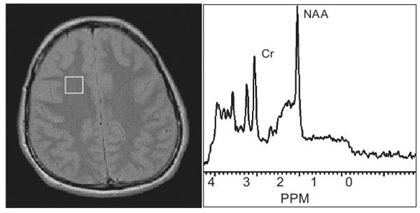
MRS voxel in the frontal white matter of HIV-infected patient and resulting MRS spectrum with the NAA and Cr peak identified.

NAA/Cr levels were available on 137 subjects (37 HIV-negative individuals - NEG, 39 HIV-positive non-symptomatic subjects - NAS, and 61 HIV-positive subjects with AIDS dementia complex - ADC). Detailed description of recruitment and cohort characteristics has been reported elsewhere [28]. In the present application, we consider the use of J₃ and VUS for classification of these subjects in the three groups, NEG, NAS and ADC, based on levels of NAA/Cr measured on each patient. It is anticipated that NAA/Cr levels will be highest among HIV-negative controls and lowest among HIV-positive neurologically impaired patients, with the NAS group being intermediate to the other two. That is, the anticipated ordering is ADC<NAS<NEG [28]. The data clearly support the normality assumption (Kolmogorov-Smirnov goodness-of-fit test conducted). As a result the Box-Cox transformation approach was not employed as it is expected that the Box-Cox approach will perform identically to the parametric approach which assumes a normal distribution of the NAA/Cr measurements. 95% confidence intervals were constructed for J₃ using the 2.5th and 97.5th quantiles of the bootstrap sample. Confidence intervals for c₁ and c₂ follow from the bootstrapped J₃ values.

Results are shown pictorially in Figure 2. From the position of the normal curves it is clear that distinguishing between the groups in terms of NAA/Cr level will be most accurate between NAS controls and ADC subjects and between NEG controls and ADC subjects, but not as much between NEG and NAS controls given the overlap of the two neurologically unimpaired groups. The estimated J₃ is slightly larger for the non-parametric approach (J₃ = 1.434, with p = 0.008, 95% CI 2.5% and 97.5% quantiles: (1.282,1.588)) compared with the parametric approach (J₃ = 1.367, with p = 0.001, 95% CI: (1.231,1.500)). The estimated cutoff c₂ is similar for the two approaches (1.990, 95% CI: (1.931, 2.046), and 1.960, 95% CI: (1.928, 1.999), respectively), but the estimated cutoff c₁ is larger for the non-parametric approach (1.830, 95% CI: (1.773, 1.888), vs 1.697, 95% CI: (1.655, 1.734)). The nonparametric VUS is equal to 0.294 (p < 0.001, 95% CI: (0.229, 0.362)), while the parametric VUS is 0.308 (p < 0.001, 95% CI: (0.246, 0.370)). We rely on the normality of the data and recommend the use of the parametric approach results in clinical practice.

Figure 2.

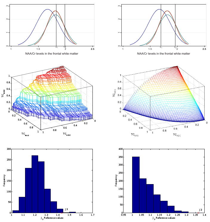
First line: Estimated normal distributions of NAA/Cr levels and optimal cutoffs according to non-parametric (left panel) and parametric (right panel) approaches. Second line: Corresponding three-dimensional ROC surface. Third line: Simulated J₃ reference distributions. The non-parametric reference distribution tends to the parametric one as the sample size increases.

5 Discussion

In this paper, we discuss J₃ as an index of diagnostic accuracy and classification into three-classes in a specific monotone ordering, such as X < Y < Z. It can be used as a complementary index to VUS, the three-dimensional generalization of the area under the ROC curve in the two-dimensional case. Non-parametric and parametric approaches were considered for estimating J₃ and the cut-points c₁ and c₂. Simulation results indicate that overall the normality assumption can be useful when normality holds or after the Box-Cox transformation for small sample sizes. J₃-based tests are suitable when location-scale differences exist. Empirical approaches can be a safe choice when normality clearly does not hold and important shape differences exist between the three distributions. In practice, both VUS and J₃ approaches can be consulted for the assessment of the discrimination between the three distributions under study. J₃ also maximizes the three-dimensional random walk height thus generalizing existing ideas [11] from two to three dimensions. In this regard, J₃ constitutes a generalization of the Kolmogorov-Smirnov test in three-class discrimination.

The non-parametric method appears to be biased for small sample sizes and when the three distributions are poorly discriminated. This happens because in these cases J₃ may not correspond to a unique point on the ROC surface but to multiple points, usually two or even three, depending on the data, a fact that holds for the Youden index too. In the simulations we have picked one ‘optimal’ operating point at random between all ‘optimal’ ones whenever this was the case. As a result, parametric methods are preferable for small sample sizes.

In the uninformative case the Youden index is J = 0 which has some intuitive appeal. However, in the uninformative case J₃ is equal to one. Both J and J₃ are defined as sums of points coordinates on the ROC curve and ROC surface respectively. Since J₃ – 1 is only a location difference it can be used instead of J₃ without any change in the essence of this work.

Application of the J₃ index in the validation of the MRS ratio NAA/Cr as a classification criterion between HIV-negative and HIV-positive control subjects and HIV-positive neurologically impaired patients led to the identification of two optimal cutoff points for this classification and showed that the classification with the NAA/Cr index is viable, and is particularly useful to distinguish between HIV-positive non-symptomatic patients and HIV-positive neurologically impaired patients. We have assumed that the reference standard used to classify patients as HIV-negative, HIV-positive neurologically unimpaired, or HIV-positive neurologically impaired is accurate. This reference standard is described in detail in [28] and has been considered as the consensus clinical diagnostic standard. A refinement of this standard has been recently proposed [29]. As the reference standard in this study may be imperfect, the methods may provide biased estimates. The issue of defining J₃ and its associated cut-off points when subjects are classified with error is a topic of future research. In the current study, the produced estimates are still relevant given that the Price & Sidtis clinical diagnostic measure is still being used. Another issue concerns the potential use of the NAA/Cr marker. Given that the use of MRS measures to diagnose HIV infection is unlikely, distinguishing between HIV-negative and HIV-positive patients, based on NAA/Cr levels, is of tertiary importance from a diagnostic perspective. However, the lack of any difference in the levels of NAA/Cr in the neurologically unimpaired groups provides significant insights into the burden of the virus on the brain and supports a two-stage model of neurological impairment where neuronal loss is a hallmark of late infection and neurological impairment. Thus, the use of NAA/Cr measured in the frontal white matter to detect HIV-associated neurological disease in HIV-infected patients is both feasible and useful.

References

- 1.Nadler JV, Cooper JR. N-acetyl- -aspartic acid content of human neural tumors and bovine peripheral nervous tissue. Journal of Neurochemistry. 1972;19:313–319. doi: 10.1111/j.1471-4159.1972.tb01341.x. [DOI] [PubMed] [Google Scholar]
- 2.López-Villegas D, Lenkinski RE, Frank I. Biochemical changes in the frontal lobe of HIV-infected individuals detected by magnetic resonance spectroscopy. Proceedings of the National Academy of Sciences of the United States of America. 1997;94:9854–9859. doi: 10.1073/pnas.94.18.9854. [DOI] [PMC free article] [PubMed] [Google Scholar]
- 3.Pepe MS. The Statistical Evaluation of Medical Tests for Classification and Prediction. Oxford University Press; 2003. [Google Scholar]
- 4.Greiner M, Pfeiffer D, Smith RD. Principles and practical application of the receiver-operating characteristic analysis for diagnostic tests. Preventive Veterinary Medicine. 2000;45:23–41. doi: 10.1016/s0167-5877(00)00115-x. [DOI] [PubMed] [Google Scholar]
- 5.Schäfer H. Constructing a cut-off point for a quantitative diagnostic test. Statistics in Medicine. 1989;8:1381–1391. doi: 10.1002/sim.4780081110. [DOI] [PubMed] [Google Scholar]
- 6.Miller R, Siegmund D. Maximally selected chi square statistics. Biometrics. 1982;38:1011–1016. [Google Scholar]
- 7.Lausen B, Schumacher M. Maximally selected rank statistics. Biometrics. 1992;48:73–85. [Google Scholar]
- 8.Lausen B, Schumacher M. Evaluating the effect of optimized cutoff values in the assessment of prognostic factors. Computational Statistics & Data Analysis. 1996;21:307–326. [Google Scholar]
- 9.Betensky RA, Rabinowitz D. Maximally selected χ2 statistics for k × 2 tables. Biometrics. 1999;55:317–320. doi: 10.1111/j.0006-341x.1999.00317.x. [DOI] [PubMed] [Google Scholar]
- 10.Hothorn T, Zeileis A. Generalized maximally selected statistics. Biometrics. 2008;64:1263–1269. doi: 10.1111/j.1541-0420.2008.00995.x. [DOI] [PubMed] [Google Scholar]
- 11.Gail MH, Green SB. A generalization of the one-sided two-sample kolmogorov-smirnov statistic for evaluating diagnostic tests. Biometrics. 1976;32:561–570. [PubMed] [Google Scholar]
- 12.Youden WJ. Index for rating diagnostic tests. Cancer. 1950;3:32–35. doi: 10.1002/1097-0142(1950)3:1<32::aid-cncr2820030106>3.0.co;2-3. [DOI] [PubMed] [Google Scholar]
- 13.Perkins NJ, Schisterman EF. The inconsistency of “optimal” cut-points using two roc based criteria. American Journal of Epidemiology. 2006;163:670–675. doi: 10.1093/aje/kwj063. [DOI] [PMC free article] [PubMed] [Google Scholar]
- 14.Fluss R, Faraggi D, Reiser B. Estimation of the youden index and its associated cutoff point. Biometrical Journal. 2005;47:458–472. doi: 10.1002/bimj.200410135. [DOI] [PubMed] [Google Scholar]
- 15.Scurfield BK. Multiple-event forced-choice tasks in the theory of signal detectability. Journal of Mathematical Psychology. 1996;40:253–269. doi: 10.1006/jmps.1996.0024. [DOI] [PubMed] [Google Scholar]
- 16.Mossman D. Three-way ROCs. Medical Decision Making. 1999;19:78–89. doi: 10.1177/0272989X9901900110. [DOI] [PubMed] [Google Scholar]
- 17.Nakas CT, Yiannoutsos CT. Ordered multiple-class ROC analysis with continuous measurements. Statistics in Medicine. 2004;23:3437–3449. doi: 10.1002/sim.1917. [DOI] [PubMed] [Google Scholar]
- 18.Nakas CT, Alonzo TA. ROC graphs for assessing the ability of a diagnostic marker to detect three disease classes with an umbrella ordering. Biometrics. 2007;63:603–609. doi: 10.1111/j.1541-0420.2006.00715.x. [DOI] [PubMed] [Google Scholar]
- 19.He X, Frey EC. Three-class roc analysis - the equal error utility assumption and the optimality of three-class roc surface using the ideal observer. IEEE Transactions on Medical Imaging. 2006;25:979–986. doi: 10.1109/tmi.2006.877090. [DOI] [PubMed] [Google Scholar]
- 20.Le CT. Evaluation of confounding effects in roc studies. Biometrics. 1997;53:998–1007. [PubMed] [Google Scholar]
- 21.Box GEP, Cox DR. An analysis of transformations. Journal of the Royal Statistical Society, Series B. 1964;26:211–246. [Google Scholar]
- 22.Burton A, Altman DG, Royston P, Holder RL. The design of simulation studies in medical statistics. Statistics in Medicine. 2006;25:4279–4292. doi: 10.1002/sim.2673. [DOI] [PubMed] [Google Scholar]
- 23.Edgington E, Onghena P. Randomization tests. 4th. Chapman & Hall / CRC; 2007. [Google Scholar]
- 24.Navia BA, Jordan BD, Price RW. The aids dementia complex: I. clinical features. Annals of Neurology. 1986;19:517–524. doi: 10.1002/ana.410190602. [DOI] [PubMed] [Google Scholar]
- 25.Navia BA, Cho ES, Petito CK, Price RW. The aids dementia complex: Ii. neuropathology. Annals of Neurology. 1986;19:525–535. doi: 10.1002/ana.410190603. [DOI] [PubMed] [Google Scholar]
- 26.Meyerhoff D, McKay S, Bahman L, Poole N, Dillon W, Weiner MW, Fein G. Reduced brain n-acetylaspartate suggests neuronal loss in cognitively impaired human immunodeficiency virusseropositive individuals: in vivo 1h magnetic resonance spectroscopic imaging. Neurology. 1993;43:509–515. doi: 10.1212/wnl.43.3_part_1.509. [DOI] [PubMed] [Google Scholar]
- 27.Meyerhoff D, McKay S, Poole N, Dillon W, Weiner MW, Fein G. N-acetylaspartate reductions measured by 1h-mrsi in cognitively impaired hiv-seropositive individuals. Magnetic Resonance Imaging. 1994;12:653–659. doi: 10.1016/0730-725x(94)92460-0. [DOI] [PubMed] [Google Scholar]
- 28.Chang L, Lee PL, Yiannoutsos CT, Ernst T, Marra CM, Richards T, Kolson D, Schifitto G, Jarvik JG, Miller EN, Lenkinski R, Gonzalez G, Navia BA. A multicenter in vivo proton-MRS study of HIV-associated dementia and its relationship to age. NeuroImage. 2004;23:1336–1347. doi: 10.1016/j.neuroimage.2004.07.067. [DOI] [PubMed] [Google Scholar]
- 29.Antinori A, Arendt G, Becker J, Brew B, Byrd D, Cherner M, Clifford D, Cinque P, Epstein L, Goodkin K, Gisslen M, Grant I, Heaton R, Joseph J, Marder K, Marra C, McArthur J, Nunn M, Price R, Pulliam L, Robertson K, Sacktor N, Valcour V, Wojna V. Updated research nosology for hiv-associated neurocognitive disorders. Neurology. 2007;69:1789–1799. doi: 10.1212/01.WNL.0000287431.88658.8b. [DOI] [PMC free article] [PubMed] [Google Scholar]