³He Lung Morphometry Technique: Accuracy Analysis and Pulse Sequence Optimization

Abstract

The ³He lung morphometry technique (Yablonskiy et al, JAP, 2009), based on MRI measurements of hyperpolarized gas diffusion in lung airspaces, provides unique information on the lung microstructure at the alveolar level. 3D tomographic images of standard morphological parameters (mean airspace chord length, lung parenchyma surface-to-volume ratio, and the number of alveoli per unit lung volume) can be created from a rather short (several seconds) MRI scan. These parameters are most commonly used to characterize lung morphometry but were not previously available from in vivo studies. A background of the ³He lung morphometry technique is based on a previously proposed model of lung acinar airways, treated as cylindrical passages of external radius R covered by alveolar sleeves of depth h, and on a theory of gas diffusion in these airways. The initial works approximated the acinar airways as very long cylinders, all with the same R and h. The present work aims at analyzing effects of realistic acinar airway structures, incorporating airway branching, physiological airway lengths, a physiological ratio of airway ducts and sacs, and distributions of R and h. By means of Monte Carlo computer simulations, we demonstrate that our technique allows rather accurate measurements of geometrical and morphological parameters of acinar airways. In particular, the accuracy of determining one of the most important physiological parameter of acinar airways – surface-to-volume ratio – does not exceed several percent. Second, we analyze the effect of the susceptibility induced inhomogeneous magnetic field on the parameter estimate and demonstrate that this effect is rather negligible at B₀ ≤ 3T and becomes substantial only at higher B₀ Third, we theoretically derive an optimal choice of MR pulse sequence parameters, which should be used to acquire a series of diffusion attenuated MR signals, allowing a substantial decrease in the acquisition time and improvement in accuracy of the results. It is demonstrated that the optimal choice represents three not equidistant b-values: b₁ = 0, b₂ ~ 2 s/cm², b₃ ~ 8 s/cm².

Introduction

Although the human (and most animal) lungs have a hierarchical branching pattern, 95% of their space resides at the acinar level where gas exchange takes place. Standard histological studies treat acinus as a conglomerate of alveoli and characterize their microstructure by means of such parameters as mean airspace chord length (L_m), lung parenchyma surface-to-volume ratio (S/V), and the number of alveoli per unit lung volume (N_a) (see for example [1]). More sophisticated (but much more labor consuming) methods allow characterizing acinus as a set of acinar airways (alveolar ducts and alveolar sacs) of cylindrical geometry with external radius R, covered by alveolar sleeve of the depth h [2, 3] – Fig. 1. The ³He lung morphometry technique, developed in our laboratory [4-6], demonstrated a great potential for evaluation of lung microstructure, based on ³He MRI measurements of inhaled gas diffusion in lung airspaces in human [6] and small animal [7] lungs. It provides information on both standard (L_m, S/V and N_a) and advanced (R and h) lung micro-geometrical parameters.

Figure 1.

Left panel: schematic structure of two levels of acinar airways. Open spheres represent alveoli forming an alveolar sleeve around each airway. Each acinar airway can be considered geometrically as a cylindrical object consisting of a tube embedded in the alveolar sleeve. Middle and right panels: two cross sections of the acinar airway model used in our simulations, with two main parameters: external radius R and depth of alveolar sleeve h. The other parameters, the internal radius r and the alveolar length L, are: r = R − h, L = 2R sinπ / 8 = 0.765 R [6].

This ³He lung morphometry technique is based on a Stejskal-Tanner pulsed field gradient [8] MRI measurements of diffusion of inhaled hyperpolarized ³He gas in lung airspaces. To establish the relationship between the measured ³He gas diffusion attenuated MR signal and lung structure, lungs should be described in terms of some basic geometrical elements. In our experiments in human lungs we selected diffusion time Δ about 1-2 ms (this should be selected shorter in small animals, like mice [7]). Given that the free diffusion coefficient of ³He gas in air, D₀ = 0.88 cm²/s, a corresponding characteristic diffusion length L₁ = (2D₀Δ)^1/2 (rms displacement in one direction) is about 0.4-0.6 mm – much larger than the average alveolar radius of 0.15 - 0.2 mm [9] but smaller than the mean length of alveolar ducts L_d (~ 0.73 mm) or alveolar sacs L_s (~1 mm) [3]. Hence, gas can diffuse out of alveoli and across the acinar airways in the time duration of the MR measurement. Under these conditions we proposed to choose acinar airways, rather than alveoli, as elementary geometrical units relevant to our experimental measurements and describe restricted diffusion of ³He atoms in each acinar airway as anisotropic, with two apparent diffusion coefficients: longitudinal, D_L, along the acinar airway axis and transverse, D_T, perpendicular to this axis [4]. In [5, 6], the apparent diffusion coefficients D_L and D_T were related to the lung morphometric parameters. Corresponding equations are also provided in the Appendix of this paper. Importantly, D_L and D_T determined from MR experiment, depend not only on lung microstructure but also on details of Stejskal-Tanner pulse sequence (diffusion attenuated gradients strength and duration [5]), hence the term “apparent”. The theory of ³He gas diffusion attenuated MR signal [4] also takes into account the fact that with current resolution of several mm, imaging voxels contain hundreds if not thousands of acinar airways of different orientations. Hence, on a macroscopic (large voxel) scale, the ³He gas diffusion attenuated MRI signal is isotropic. The diffusion attenuated MR signal from a voxel containing a multitude of airways oriented equally in all directions is a sum of signals from individual airways and is described as follows [4]:

$$S(b)=S_0\exp (-b{D}_T){\left(\frac{\pi }{4b(D_L-D_T)}\right)}^{1/2}·\mathrm{\Phi }[{(b(D_L-D_T))}^{1/2}],$$ (1)

where Φ is the error function, the apparent diffusion coefficients D_L and D_T are defined by Eqs. (13), (14), (16), (17) in the Appendix and b-value is defined by Eq. (4). Thus, our technique incorporates the salient feature of gas diffusion in acinar airways on the time scale of a few milliseconds, namely, its microscopically anisotropic but macroscopically isotropic character. This prediction of our theory and validity of Eq. (1) was confirmed in vivo by experimental measurements in humans [4, 6], canines [10], mice [7] and especially for a broad range of b-values (up to 40 s/cm²) in rats [11].

The ³He lung morphometry technique is to fit Eq. (1) to a multi-b value measurement of a diffusion-attenuated MR signal using Eqs. (13), (14), (16), (17) in the Appendix that connect the apparent diffusion coefficients D_L and D_T to parameters R and h. Thus, R and h and amplitude S₀ are the only fitting parameters. Other physiological quantities of interest (surface-to-volume ratio S/V, mean chord length L_m, alveolar density N_a) can then be calculated [6]:

$$\begin{array}{c}S/V=\frac{2\pi R·L+2\pi ·(R^2-r^2)+16(R-r)·L}{\pi R^{2}L},L=2R\sin \frac{\pi }{8}=0.765R\\ L_m=4·V/S,N_a=1/(\pi R^{2}L)\end{array}$$ (2)

Comparison of these parameters obtained in human lungs by means of the ³He lung morphometry technique and those found by direct histological measurements has revealed very good agreement [6], thus providing direct validation of the proposed ³He lung morphometry technique.

As already mentioned above, our model incorporates the salient feature of gas diffusion in acinar airways on the time scale of a few milliseconds (human lungs), namely, its microscopically anisotropic but macroscopically isotropic character. However, as any model mimicking a complicated structure, it is based on assumptions and simplifications that might bias the measurements. In this manuscript, computer Monte-Carlo simulations are used to simulate the MR signal S_sim(b) in the “expanded” model accounting for (a) the branching structure of the acinar airways and the finite length of alveolar ducts and sacs, (b) the distribution of airway geometrical parameters R and h, and (c) the effects of internal inhomogeneous magnetic fields. We will fit then the simulated signal S_sim(b) by our original method [6] – using Eq. (1) with the apparent diffusion coefficients D_L and D_T defined by Eqs. (13), (14), (16), (17) in the Appendix and see how well the measurement method recovers the parameters R and h used in the simulations. We will also address some other details related to derivation of our theoretical model.

Besides, we will answer the important question: what is the best choice of b values to optimize the accuracy and precision of the S/V measurement? For this purpose, we will use the Bayesian probability theory and minimize the variance of the S/V statistic with respect to b-values.

Methods – Lung Model and Computer Monte-Carlo simulations

Generally, to analyze the MR signal in an acinus by means of computer simulations, one might want to “construct” a complete model of the acinus with numerous airway generations included. However, as follows from our simulations, in the range of diffusion times Δ used in our experiments in human lungs (1.8 ms), most of the particles which originate (i.e. start their random walk) in any given airway will remain in the initial airway or move to (essentially) only one adjacent airway. The probability to reach the next branching node and to diffuse into the next-to-adjacent airway is negligibly small. That is why the signal from the ³He atoms originating in one airway (duct or sac) does not depend on whether the adjacent airways are ducts or sacs. Moreover, these adjacent airways can be considered infinitely long, ignoring their branching because of the extremely low probability of a diffusing atom reaching the “next branching node”. Of course, such a simplification is not valid for long diffusion times. Thus, it is sufficient for our diffusion times to consider only two different simplified airway configurations as shown in Fig. 2.

Figure 2.

Two airway configurations used in computer simulations. The internal alveolar structure of the airways is not shown and the aspect ratio is changed for better view of the structures. The highlighted airway (grey shading) at left is an airway duct and at right an airway sac.

The first configuration with two nodes (Fig. 2a) corresponds to an alveolar duct of generation Z (shaded horizontal airway in Fig. 2a), surrounded by a “parent” duct of generation (Z − 1), a “sister” airway of generation Z, and two “daughter” airways of generation (Z + 1). In what follows, we assume symmetrical branching with half-angle α, a “parent” and its “daughter” airways being co-planar. Virtually no atoms sample airways on both sides of the central, shaded airway, so the relative orientation of the two planes (to left and right of the central airway) is not important. The second configuration with one node (Fig. 2b) corresponds to an alveolar sac of terminal generation Z (shaded horizontal airway in Fig. 2b), surrounded by a “parent” duct of generation (Z − 1) and a “sister” airway of generation Z.

The branching angle α characteristic of acinar airways is experimentally unknown so far. However, according to microphotographs in [12], this angle is smaller than in conducting airways. For the latter, we can speculate that the branching angle should be similar to that for arterial blood vessels analyzed in [13], where it was found that 2α resides in the interval 75-90°. Obviously, the effect of branching on the MR signal formation increases with increasing α (if the angle α is 0, the branching plays no role at all). In our simulations, we choose α = 40° to provide estimates for the accuracy of our approach, corresponding to a worst case scenario.

We calculate signals from ducts and sacs separately. For this purpose, 10⁶ particles are uniformly generated within the “main” airway (shaded in Fig. 2) and then allowed to randomly walk within one of the structures shown in Fig. 2. According to [3], the number of ducts N_d and sacs N_s is approximately the same, N_d = N_s (this is a property of a binary tree). However, the average lengths of ducts and sacs are different: L_d = 0.73 mm and L_s = 1 mm [3], corresponding approximately to the size of 3 and 4 alveoli, respectively. Thus, the lengths of the “main” duct and sac in the simulations are chosen to be 3L and 4L, respectively (with L defined in Fig. 1). To account for a distribution of airway geometrical parameters and the distribution of the orientations, the following sampling was adopted for each generated particle:

• - the geometrical parameters of the airways (R and r) were chosen according to Gaussian distributions centered at R₀ and r₀ with STD of 17% of the mean values [3].

• - the orientation of the “main” airway with respect to the external field gradient G, as well as the orientations of the planes spanning the airways corresponding to the nodes in Fig. 2, were chosen randomly.

Such a procedure leads to self-averaging of the signal with respect to the aforementioned orientations and distribution of airway geometrical parameters. The total normalized MR signal can be calculated as a weighted sum of normalized signals from the particles generated in ducts (s_d) and sacs (s_s):

$$S_{\mathit{sim}}=(3s_d+4s_s)/7.$$ (3)

The details of computer simulations of random-walks were fully described in [5]. At each computer step of duration Δt = 10⁻³ ms, a particle moves with equal probability in one of 8 directions (±1, ±1, ±1) over distance l₀ = (6D₀ · Δt)^1/2, where D₀ = 0.88 cm²/s is the free diffusion coefficient of ³He gas in N₂ or air. At each step j of a random walk through the magnetic field gradient, a particle gains a spin precession phase Δψ_j = γG(t_j) · r(t_j) · Δt, where r(t_j) is the position of the particle at step j, and G(t_j) is the time-dependent magnetic field gradient used for diffusion encoding. The index j enumerates computer time steps running from 0 to N = T / Δt, where T is the full sequence time and t_j = j · Δt. If a contemplated jump would pass through any boundary (see Fig. 1), the move is rejected and the particle remains at the initial position. The MR signal from each particle is equal to exp(iψ), $\psi =\sum _{j=0}^N\mathrm{\Delta }{\psi }_j$.

Our diffusion measurements use the Stejskal-Tanner pulsed field gradient experiment [8] in which a free-induction decay MR signal is interrupted by two opposite-polarity diffusion-sensitizing gradient pulses characterized by the so-called b-value. For the gradient waveform selected in our experiment [4], the b-value is:

$$b={(\gamma G_m)}^2\left[{\delta }^2\left(\mathrm{\Delta }-\frac{\delta }{3}\right)+\tau \left({\delta }^2-2\mathrm{\Delta }\delta +\mathrm{\Delta }\tau -\frac{7}{6}\delta \tau +\frac{8}{15}{\tau }^2\right)\right]$$ (4)

where γ is nuclear gyromagnetic ratio, G_m is the gradient lobe amplitude, Δ is the spacing between the leading edges of the positive and negative lobes, δ is the duration of each lobe, and τ is a ramp-up and ramp-down time. Typical values of these parameters used in our experiments are Δ = δ = 1.8 ms, and τ = 0.3ms. In simulations, we use Δ = δ = 1.8 ms, τ = 0. The sequence timing parameters are kept constant and the b-value, Eq.(4), is altered from 0 to 10 s/cm² by changing the gradient amplitude G_m.

The signal S_sim(b), Eq. (3), calculated for a set of the input parameters R₀ and r₀ is then fitted (χ² – minimization) by our model, Eq.(1) with the apparent diffusion coefficients D_L and D_T defined by Eqs. (13), (14), (16), (17).

Results and Discussion

Branching effects, finite length of alveolar ducts and sacs, the distribution of airway geometrical parameters R and h

The input values of the geometrical parameters (typical for healthy lungs and lungs with mild emphysema) used in our simulations and those found from the model (fitting parameters) are presented in Table 1. The numbers in parenthesis represent the relative difference (in %) between the value found from the analysis and the corresponding input value. In Table 1, the value of surface-to-volume ratio S/V. is also included.

Table 1.

Results obtained for lung acinar airway structure depicted in Fig. 2 with α = 40° and parameters R and r distributed according to Gaussian distributions centered at R₀ and r₀ with STD of 17% of the mean values [3]. The numbers in parenthesis represent the relative difference (%) between the value found from the fitting analysis and the corresponding input value.

input parameters			fitting parameters
R0, μm	r0, μm	(S/V)0, cm-1	R, μm	r, μm	S/V, cm-1
300	140	225	286 (-5%)	135 (-4%)	235 (4%)
300	180	190	296 (-1%)	163 (-9%)	210 (8%)
350	180	183	314 (-10%)	171 (-5%)	196 (7%)
350	220	156	330 (-6%)	199 (-9%)	172 (9%)

According to Table 1 all the parameters (R, r, S/V) found from fitting the model to simulated data using Eq. (1) with D_L and D_T defined by Eqs. (13), (14), (16), (17), representing an idealized structure of branching acinar airways, are very close to the input values. In particular for the surface-to-volume ratio, the average difference is 6.5% and does not exceed 11%. We also added Gaussian noise to the simulated data (SNR=100), and found practically no difference in output values. It means that for SNR equal or bigger than 100 fitting differences associated with noise are much smaller than that related to other sources. Note also that in our experiments, SNR is usually much higher than 100.

One of the main assumptions of our model was the ability to describe the total MR signal from an acinus as the sum of signals from individual acinar airways. This assumption holds only if a diffusing ³He atom resides primarily within the same airway throughout the diffusion gradient pulse. As our diffusion times are smaller than the characteristic time to diffuse the length of an airway, this might happen in two ways. First, a particle might spend all or most of the time in the same airway where it originated; most likely these are particles that originate near the center of the airway or ones that originate around one airway end and diffuse toward the other end. Second, particles can originate near the airway open end, diffuse into the adjacent airway and perform most of their random walk there. Our simulations demonstrate that indeed, most walkers spend most of their diffusion time (typically, 75%) within a single airway. This explains why our approach, based on the assumption of “non-communicating” airways, describes data very well, as shown in Table 1.

Non-Gaussian Effects in the Theory of ³He Lung Morphometry Technique

Our previous Monte-Carlo simulations [5] demonstrated that for a single acinar airway MR signal dependence on b-value deviates from monoexponential behavior but for the moderate b-values used in most experiments (up to 10-12 s/cm²), the MR signal can be well described by the second-order cumulant expansions when diffusion gradient is oriented either parallel or perpendicular to an acinar airway axis, see Eqs. (12), (13), (15), and (16). These expressions include terms of order b and b² in the exponential. That is often called kurtosis approximation (see for example [14]). The dependence of the apparent diffusion coefficients D_L(b) and D_T(b) on b-value in Eqs. (5) and (1) reflects non-Gaussian effects that are always present in diffusion attenuated MR signal in case of restricted diffusion (see for example discussion in [15]). In our approach [5, 6] we have made an assumption that for an arbitrary orientation of the acinar airway with respect to the diffusion gradient, characterized by angle θ, the signal can be described by the following equation:

$$S(b;\theta )=S_0·\exp \left\{-b\left[D_L(b){\cos }^2\theta +D_T(b){\sin }^2\theta \right]\right\}$$ (5)

where apparent diffusion coefficients D_L(b) and D_T(b) are given in Eqs. (13) and (16). Then, the diffusion attenuated MR signal from a voxel containing a multitude of uniformly oriented airways is a sum of signals from individual airways [4], resulting in Eq. (1).

Strictly speaking, for arbitrary angle θ the second order cumulant expansion in Eq. (5) contains a small additional term in the exponent, proportional to b² sin²θ cos²θ. This term, however, contributes only within a rather narrow interval about θ ~ π/4 and therefore would have a small effect on the total signal from a voxel comprised of a multitude of airways with different orientations in Eq. (1). At the same time, its inclusion could unjustifiably complicate the analytical expression for the MR signal in Eq. (1). Thus, this term is omitted in our approach.

To demonstrate that the effect of this term on the total signal from a multitude of uniformly oriented airways is really small, we simulated the signal S_sim(b) in a system of infinite-length airways (no branching, no sacs, no internal fields) and compared it with the signal calculated by our standard approach (Eq. (1) and associated Eqs. (13), (14), (16), (17) in Appendix), identical to Eqs. A1-A5 in [6]. The results are presented in Fig. 3 for the same input parameters R₀ and r₀ as in Table 1. These results demonstrate that even for b = 10 s/cm², there is a very good agreement between the simulated and calculated signals. We note that the curves in Fig. 3 are not the fitting results with adjustable R and r but calculations with the same input parameters as simulations. When we do fit Eq. (1) and associated Eqs. (13), (14), (16), (17) (or Eqs. A1-A5 in [6]) to these generated data, we find fitting parameters that are very close to the input parameters. The average errors are about 3% and 4% for parameters R and r, correspondingly.

Figure 3.

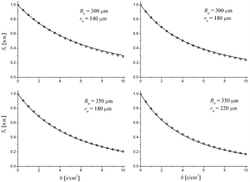
Examples of diffusion attenuated MR signals from a random distribution of acinar airways: symbols - simulated signals; curves - signals calculated using Eq. (1) with D_L and D_T defined by Eqs. (13), (14), (16), (17).

Recently Parra-Robles et al [16] argued about the theoretical basis of our technique. Based on their experimental results obtained on phantoms, they stated that our results “are not valid for large diffusion gradient strengths (above 15 mT/m), which are commonly used for ³He ADC measurements in human lungs”. Note that for diffusion time of 1.8 ms, used in our simulations and measurements, b = 10 s/cm² corresponds to gradient strength G_m ~ 30 mT/m – twice as large as the number claimed by Parra-Robles et al as the threshold for break-down of our model. Our results demonstrated in Fig. 3 show that conclusions made by Parra-Robles et al [16] based on phantom experiments are not applicable to our method.

Effects of Internal field gradients

In the presence of magnetic field B₀, lung parenchyma becomes weakly magnetized, creating a secondary inhomogeneous magnetic field in the lung airspaces. This field depends on the geometry of the septa forming alveoli and the susceptibility difference Δχ between the septa and the lung airspaces. In the model of acinar airways shown in Fig. 1, there are three types of septa in each airway, i.e. external cylindrical surface with radius R, transverse rings with external and internal radii R and r, respectively, and planes of width h = R − r, parallel to the airway axis. For all these shapes the magnetic field can be calculated analytically by solving Maxwell’s equations in the small-susceptibility limit and taking into account that the thickness of alveolar septa, d, is much smaller than R and r. We are interested in the component of this field parallel to the external magnetic field B₀. Ignoring effects of finite airway length, we first note that the cylindrical surface does not create secondary field inside the airway. The contribution from the rings, B_r, is as follows:

$$\begin{array}{l}{B}_r={\displaystyle \sum _{j=-\infty }^{\infty }\left[B_{\rho }^{(j)}\left(x{n}_x+y{n}_y\right)/\rho +B_z^{(j)}{n}_z\right]}\\ B_{\rho }^{(j)}=B_0{n}_{z}d\mathrm{\Delta }\chi ·\left[F_{\rho }\left(\rho ,z_j,R\right)-F_{\rho }\left(\rho ,z_j,r\right)\right]\\ B_z^{(j)}=B_0{n}_{z}d\mathrm{\Delta }\chi ·\left[F_z\left(\rho ,z_j,R\right)-F_z\left(\rho ,z_j,r\right)\right]\\ F_{\rho }\left(\rho ,z_j,a\right)=\frac{z_j}{\rho }{\left(\frac{m_a^{(j)}}{a\rho }\right)}^{1/2}\left[\frac{\left(a^2+{\rho }^2+z_j^2\right)}{{(a-\rho )}^2+z_j^2}·\mathbf{E}(m_a^{(j)})-\mathbf{K}(m_a^{(j)})\right]\\ F_z\left(\rho ,z_j,a\right)={\left(\frac{m_a^{(j)}}{a\rho }\right)}^{1/2}\left[\frac{\left(a^2-{\rho }^2-z_j^2\right)}{{(a-\rho )}^2+z_j^2}·\mathbf{E}(m_a^{(j)})+\mathbf{K}(m_a^{(j)})\right]\\ m_a^{(j)}=\frac{4a\rho }{{\left(a+\rho \right)}^2+z_j^2},\rho ={(x^2+y^2)}^{1/2},z_j=z-\mathit{jL}\end{array}$$ (6)

Here (x, y, z) are Cartesian coordinates with the origin at the center of one of the rings with the z axis parallel to the airway axis; (n_x,n_y,n_z) are projections of the unit vector parallel to the main magnetic field B₀; K(m) and E(m) are the complete elliptic integrals of the first and second kind, respectively. Although the sum over j is formally from −∞ to +∞, it converges very fast and the terms corresponding to the smallest z_j play the main role.

The contribution from the planes, B_p, depends only on the position in the transverse direction with respect to the airway axis, and is defined by the two-dimensional vector ρ = (x, y), and is given by

$$\begin{array}{c}{B}_p=2B_{0}d\mathrm{\Delta }\chi ·\sum _{j=1}^8\left(n_y\cos {\phi }_j-n_x\sin {\phi }_j\right)·\left[U(\mathbf{\rho }-R{\mathbf{q}}_j)-U(\mathbf{\rho }-r{\mathbf{q}}_j)\right]\\ U(\mathbf{a})=\frac{1}{a^2}\left(a_y{n}_x-a_x{n}_y\right),{\mathbf{q}}_j=(\cos {\phi }_j,\sin {\phi }_j)\end{array}$$ (7)

where the sum is over 8 angles, φ_j = {0, π / 4, π / 2, …, 7π / 4}.

The effect of the susceptibility induced inhomogeneous magnetic fields is analyzed assuming that Δχ = 0.72 ppm (as for water/air interface, CGS units) and the septa thickness d = 10 μm [17, 18]. The computer Monte-Carlo simulations were performed in the same way as described above but now the phase φ accumulated by diffusing particles was calculated accounting for both the external gradient and the internal inhomogeneous field B_r + B_p. It should be noted that the signal attenuation due to the internal field gradients starts immediately after the RF pulse (some time before the first gradient lobe) and continues after the second gradient lobe. That is why its total duration, T_f, is longer than the duration of external gradients Δ + δ. In our simulations, we choose these parameters according to the experimental protocol used in our previous studies [4-6]: T_f = 7.2 ms, Δ + δ = 3.6 ms. The signal S(b) (simulated for R₀ = 300 μm, r₀ = 140 μm) is analyzed by means of our model, Eq. (1). The results for the “apparent” parameters R and r, as well as for the surface-to-volume ratio, are presented in Table 2. The numbers in parenthesis represent the relative difference (in %) between the values found from the simulation data obtained with B₀ ≠ 0 and the corresponding values obtained when the internal field is absent (values given in the first row of Table 2).

Table 2.

Effect of internal field gradients. Fitting results for simulated data at different external field B₀. The numbers in parenthesis represent the relative difference (%) between the values found from the simulation data obtained with and without internal field gradients.

	fitting parameters
B0, T	R, μm	r, μm	S/V, cm-1
0	317	136	222
1.5	316 (-0.2%)	138 (1%)	221 (-0.3%)
3	315(-0.6%)	141 (4%)	219 (-1.4%)
4.7	314 (-0.7%)	150 (10%)	212 (-4%)
7	325 (3%)	181 (33%)	186 (-16%)

According to Table 2, the effect of the internal inhomogeneous field on the most important morphological parameter – surface-to-volume ratio - is rather negligible at B₀ = 1.5T; the effect increases as B₀ increases, reaching 16% at B₀ = 7T. Thus, experiments with high B₀ can distort the fitting parameters and, of course, do not increase SNR for hyperpolarized gas [19].

Optimization of b-values

Important practical questions also include (a) how does noise in the experimental data affect estimation of model parameters and (b) what is the optimal choice of experimental sequence parameters for obtaining the best possible parameter estimate (given restricted imaging time, typically, a 10-second breathhold). Herein we provide estimates of the optimal b-values that allow evaluation of lung geometrical parameters with minimal errors based on the method similar to [20]. We use Bayesian analysis [20, 21] to examine how the estimated geometrical parameters R and r depend on their “true values”, signal-to-noise ratio, and data sampling (that is, the b-values). To achieve the maximum lung coverage in an experimental setting with restricted data acquisition time, the number N of b-values should be chosen to be as few as possible (N = 3 in our case because the data is characterized by 3 parameters: S₀, R, and h, as in Eq. (1) with D_L and D_T defined by Eqs. (13), (14), (16), (17)). Here we demonstrate that the smallest uncertainty in parameter estimates can be achieved by using a set of unequally spaced b-values.

The basic quantity in Bayesian analysis is a joint posterior probability P({p_j}|Data, σ, I) for model parameters {p_j} given all of the data Data, the noise standard deviation σ, and the prior information I. In the high signal-to-noise approximation [21]

$$P\left(\{p_j\}|\mathit{Data},\sigma ,I\right)\propto \exp \left(-Q/2{\sigma }^2\right)$$ (8)

where $Q=\sum _{n=0}^{N-1}{\left[\widehat{S}(b_n)-S(b_n)\right]}^2$. Here the function Ŝ(b_i) represents Data and is determined from the model S(b_i) (Eq. (1) with D_L and D_T defined by Eqs. (13), (14), (16), (17)) by substitution of the parameters p_i = {R, h, S₀} with their “true” values p̂_i. To estimate any parameter in the model, a posterior probability for the parameters should be calculated, from which the estimated values of the parameters can be found in the form:

$${\left(p_j\right)}_{\mathit{est}}={\widehat{p}}_j\pm \delta p_j,\delta p_j={\mathit{SNR}}^{-1}·{\left({\mathrm{\Delta }}_j/\mathrm{\Delta }\right)}^{1/2},$$ (9)

where δp_j are the expected uncertainties of the estimated parameter SNR = Ŝ₀ / σ signal-to-noise ratio; Δ is the determinant of the variance-covariance matrix A with the rank M equal to the number of model parameters, and Δ_j is the minor of this matrix corresponding to the diagonal element jj. The matrix elements of A are determined by the derivatives of the function S(b_n):

$$A_{\mathit{ij}}=\sum _{n=0}^{N-1}{S}_i(b_n)S_j(b_n),S_i={\left(\partial S/\partial p_i\right)}_{p_i={\widehat{p}}_i}$$ (10)

Optimal parameters of the pulse sequence correspond to a set of b-values minimizing the expected uncertainties δp_j. Obviously, the number of b-values N cannot be smaller than the number of the model parameters M, (if N < M, the determinant Δ = 0, and all the uncertainties δp_j → ∞). Here we restrict our analysis to the case of a minimal number of b-values (N = 3), allowing estimation of three parameters in the model given by Eq. (1) with D_L and D_T defined by Eqs. (13), (14), (16), (17): the signal amplitude S₀ and two geometrical parameters of the acinar airways, R and r. Equations (9)-(10) make it possible to estimate not only the expected uncertainties of these parameters but the expected uncertainties of the derivative parameters, i.e. the surface-to-volume ratio S / V, as well. The expected uncertainty of the latter can be found by making use of Eq. (11):

$$\delta (S/V)={\left[{\left(\frac{\partial (S/V)}{\partial R}\right)}^2{\left(\delta R\right)}^2+{\left(\frac{\partial (S/V)}{\partial r}\right)}^2{\left(\partial r\right)}^2\right]}^{1/2}$$ (11)

The optimal set of b-values, resulting in the best parameter estimates, corresponds to the minimum of δp_j in Eq. (11). One of the optimal b-values is found to be b₀ = 0; two others will be denoted as b₁ and b₂. Obviously, the set of optimal b₁ and b₂ depends on the targeted estimated parameter. In what follows, we consider optimization with respect to the most important morphological parameter, S / V.

An analysis of δ(S / V) in Eq. (11) (not detailed here) demonstrates that for typical values of R and r for human lungs, the optimal b₁ resides in a narrow interval from 2 to 3 s/cm², whereas the optimal b₂ is rather high, from 12 to 20 s/cm², as shown in Fig. 4a. Such high b-values require strong diffusion-sensitizing gradients which are not always available and assume a sufficiently high SNR to accurately measure the strongly-attenuated signal at these b-values. Fortunately, the b₂-dependence is rather weak; therefore, nearly the same quality of parameter estimates can be achieved with slightly smaller than optimal b² values.

Figure 4.

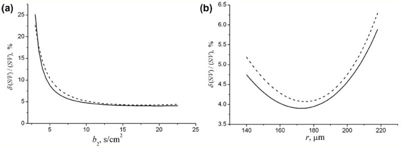
(a) The dependence of the relative uncertainty estimate of the surface-to-volume ratio, ε = δ (S / V) / (S / V), on b₂ in the 3b experiment for R = 300 μm, r = 140 μm, and SNR = 100; b₁ = 2 s/cm². (b) The dependence of ε on the internal radius r at R = 300 μm, SNR = 100, b₁ = 2 s/cm², b₂ = 10 s/cm². The dashed curves in (a) and (b) corresponds to ε in the 6b experiment with equidistant b-values (0, b₂ / 5, 2b₂ / 5, …, b₂).

The dependence of the relative uncertainty estimate, ε = δ(S / V) / (S / V), on b₂ is shown in Fig. 4a (solid line) for b₁ = 2 s/cm² and acinar airway parameters typical of healthy lungs, R = 300 μm, r = 140 μm, and SNR = 100. This graph demonstrates that the parameter ε dramatically decreases as b₂ increases up to 7–8 s/cm² and remains practically flat for higher b-values. The relative errors in the parameter estimates corresponding to b₂ > 8 s/cm² do not exceed 5% at this SNR. Thus, in real experiments, the optimal choice of b-values is a compromise between the best estimates of the desired parameters and hardware restrictions on gradient strength.

As already mentioned above, the set of optimal b₁ and b₂ depends on the targeted estimated parameter. For example, the best choice of b-values in the 3b experiment corresponding to optimizing the parameter R or r is, generally speaking, different from that corresponding to S/V. However, a numerical analysis demonstrates that the dependencies of the relative uncertainty estimates for R or r, ε_R = δR / R and ε_r = δr / r, on b₁ and b₂ are very similar to that of the parameter ε, discussed above: for both these parameters, the optimal b₁ resides in a narrow interval from 2 to 3 s/cm², whereas ε_R and ε_r dramatically decreases as b₂ increases up to 7–8 s/cm² and remains practically flat for higher b-values. Thus, the compromise choice of b-values for ε_R and ε_r is the same as for the parameter ε: b₁ = 2 – 3 s/cm² and b₂ = 7–8 s/cm².

The optimum choice of the three b-values has a clear physical basis. The b₀ = 0 measurement obviously establishes the value of S₀ in Eq. (1). The value b₁ = 2 – 3 s/cm² results in e-fold attenuation of the factor in Eq. (1), depending on D_an = D_L − D_T, given that D_an is approximately 0.3 s/cm² for our chosen parameters. The larger b₂ serves to establish D_T, the parameter describing the most slowly decaying component in the signal – the exponential factor in Eq. (1) (D_T is approximately 0.07 s/cm² for our chosen parameters). It should be noted that if, for some reason, the maximal b-value is chosen to be not high enough, the uncertainty in parameter estimate will be much higher due to insufficient dynamic range.

For comparison, similar relative errors are shown (dashed lines) for experiments with 6 equidistant b-values (0, b₂ / 5, 2b₂ / 5, …, b₂) and SNR = 100/√2 (decrease in SNR by the factor √2 is due to the decreased flip angle necessary to acquire twice as many b-values). As we see, for the same maximum gradient, the 3b-value pulse sequence with non-equidistant optimized b-values results in slightly smaller uncertainties of the estimated parameters than the 6b-value pulse sequence. Importantly, the 3b-value pulse sequence also requires only half the time as compared to a 6b-value pulse sequence.

The results shown in Fig. 4a correspond to acinar airways typical of the healthy lungs. In mild emphysema the external airway radius R slightly increases whereas the internal radius r increases substantially [6]. Figure 4b illustrates the dependence of the relative error of S/V on the internal radius r for R = 300 μm. The relative error of the external radius R monotonically decreases (not shown), whereas that of the internal radius r has a minimum at r = 170 μm.

Thus, in the range of acinar airway parameters corresponding to healthy lungs and lungs with initial stages of emphysema, the optimized 3b-value pulse sequence results in smaller relative errors in the parameter estimates than can be achieved by means of the twice longer 6b-value pulse sequence with equidistant sampling. This reduced imaging time can be harnessed to decrease the duration of breath-hold or to increase the number of acquired slices.

Conclusions

In this study, we analyze the accuracy of the MRI-based ³He lung morphometry technique [4-6]. The initial works with the ³He lung morphometry technique approximated the acinar airways as very long cylinders, all with the same radii R and r. The present work aims at analyzing effects of realistic acinar airway structures, incorporating airway branching, physiological airway lengths, a physiological ratio of airway ducts and sacs, and distributions of airway radii R and r. Analysis of the signals simulated in this way, using the model equations, returns values of R, r, and S/V in good agreement with the input parameters of the simulations. Thus, the approximations that the initial work was based upon are quite justified and in a practical sense, the results of the ³He lung morphometry technique are no longer dependent upon these assumptions. We also demonstrate that the effect of the susceptibility induced inhomogeneous magnetic field on the parameter estimate is negligible at currently used field strength, up to 4.7T. Finally, we derive an optimal choice of MR pulse sequence parameters, which should be used to acquire a series of diffusion attenuated MR signals, allowing substantial decrease in the acquisition time and improvement in accuracy of the results.

Appendix

Our previous Monte-Carlo simulations [5] demonstrated that for a single acinar airway MR signal dependence on b-value deviates from monoexponential behavior but for the moderate b-values used in most experiments (up to 10-12 s/cm²), the MR signal can be well described by the second-order cumulant expansion. In particular, if the diffusion sensitizing gradient G is oriented along the airway, the MR signal is

$$S_L(b)=S_0\exp \left[-b{D}_L(b)\right]$$ (12)

where the apparent longitudinal diffusion coefficient depends on b:

$$D_L(b)=D_{L0}·(1-{\beta }_L·b{D}_{L0})$$ (13)

This expression includes terms of order b and b² in the exponential, that is often called kurtosis approximation (see for example [14]). In [6], the parameters D_L0 and β_L were related to the main geometrical parameters of the acinar airways R and h defined in Fig. 1:

$$D_{L0}=D_0·\exp \left[-2.89·{(h/R)}^{1.78}\right],{\beta }_L=35.6·{(R/L_1)}^{1.5}·\exp \left[-4/\sqrt{h/R}\right]$$ (14)

When the diffusion sensitizing gradient G is oriented perpendicular to the airway, the MR signal has a similar form:

$$S_T(b)=S_0\exp \left[-b{D}_T(b)\right]$$ (15)

where apparent transverse diffusion coefficient is

$$D_T(b)=D_{T0}·(1+{\beta }_T·b{D}_{T0})$$ (16)

The parameter D_T0 is also related to R and h [6]:

$$\begin{array}{c}{D}_{T0}=D_0·\exp \left[-0.73·{(L_2/R)}^{1.4}\right]·[1+f(R,h)]\\ f(R,h)=\exp \left(-A·{(h/R)}^2\right)·\left[\exp \left(-5{(h/R)}^2\right)+5·{(h/R)}^2-1\right]\\ A=1.3+0.25·\exp \left[14·{(R/L_2)}^2\right]\\ L_2={(4D_0\mathrm{\Delta })}^{1/2},{\beta }_T=0.06\end{array}$$ (17)

Equations (12) - (17) are obtained as empirical descriptions of the results of computer Monte-Carlo simulations (see details in [5, 6]). These equations are valid for the diffusion time Δ in the millisecond range and for alveolar parameters typical of healthy human lungs and lungs with mild emphysema, R ~ 300 – 400 μm, h / R < 0.6 [3].

References

- 1.Hsia CC, Hyde DM, Ochs M, Weibel ER. An official research policy statement of the American Thoracic Society/European Respiratory Society: standards for quantitative assessment of lung structure. Am J Respir Crit Care Med. 2010;181:394–418. doi: 10.1164/rccm.200809-1522ST. [DOI] [PMC free article] [PubMed] [Google Scholar]
- 2.Rodriguez M, Bur S, Favre A, Weibel ER. Pulmonary acinus: geometry and morphometry of the peripheral airway system in rat and rabbit. Am J Anat. 1987;180:143–155. doi: 10.1002/aja.1001800204. [DOI] [PubMed] [Google Scholar]
- 3.Haefeli-Bleuer B, Weibel ER. Morphometry of the Human Pulmonary acinus. The anatomical Record. 1988;220:401–414. doi: 10.1002/ar.1092200410. [DOI] [PubMed] [Google Scholar]
- 4.Yablonskiy DA, Sukstanskii AL, Leawoods JC, Gierada DS, Bretthorst GL, Lefrak SS, Cooper JD, Conradi MS. Quantitative in vivo assessment of lung microstructure at the alveolar level with hyperpolarized 3He diffusion MRI. Proc Natl Acad Sci U S A. 2002;99:3111–3116. doi: 10.1073/pnas.052594699. [DOI] [PMC free article] [PubMed] [Google Scholar]
- 5.Sukstanskii AL, Yablonskiy DA. In vivo lung morphometry with hyperpolarized (3)He diffusion MRI: Theoretical background. J Magn Reson. 2008;190:200–210. doi: 10.1016/j.jmr.2007.10.015. [DOI] [PMC free article] [PubMed] [Google Scholar]
- 6.Yablonskiy DA, Sukstanskii AL, Woods JC, Gierada DS, Quirk JD, Hogg JC, Cooper JD, Conradi MS. Quantification of lung microstructure with hyperpolarized 3He diffusion MRI. J Appl Physiol. 2009;107:1258–1265. doi: 10.1152/japplphysiol.00386.2009. [DOI] [PMC free article] [PubMed] [Google Scholar]
- 7.Osmanagic E, Sukstanskii AL, Quirk JD, Woods JC, Pierce RA, Conradi MS, Weibel ER, Yablonskiy DA. Quantitative Assessment of Lung Microstructure in Healthy Mice using an MR-based 3He Lung Morphometry Technique. J Appl Physiol. 2010 doi: 10.1152/japplphysiol.00736.2010. [DOI] [PMC free article] [PubMed] [Google Scholar]
- 8.Stejskal EO. Use of Spin Echoes in a Pulsed Magnetic-Field Gradient to Study Anisotropic, Restricted Diffusion and Flow, Jour. Chem Phys. 1965;43:3597–3603. [Google Scholar]
- 9.Ochs M, Nyengaard JR, Jung A, Knudsen L, Voigt M, Wahlers T, Richter J, Gundersen HJ. The number of alveoli in the human lung. Am J Respir Crit Care Med. 2004;169:120–124. doi: 10.1164/rccm.200308-1107OC. [DOI] [PubMed] [Google Scholar]
- 10.Tanoli TS, Woods JC, Conradi MS, Bae KT, Gierada DS, Hogg JC, Cooper JD, Yablonskiy DA. In vivo lung morphometry with hyperpolarized 3He diffusion MRI in canines with induced emphysema: disease progression and comparison with computed tomography. J Appl Physiol. 2007;102:477–484. doi: 10.1152/japplphysiol.00397.2006. [DOI] [PMC free article] [PubMed] [Google Scholar]
- 11.Jacob RE, Laicher G, Minard KR. 3D MRI of non-Gaussian 3He gas diffusion in the rat lung. J Magn Reson. 2007;188:357–366. doi: 10.1016/j.jmr.2007.08.014. [DOI] [PubMed] [Google Scholar]
- 12.Albertine KH. In: Application of Magnetic Resonance to the Study of Lung. Cutillo AG, editor. Futura Publishing Company, Inc.; Armonk, NY: 1996. pp. 73–114. [Google Scholar]
- 13.Murray CD. The Physiological Principle of Minimum Work Applied to the Angle of Branching of Arteries. J Gen Physiol. 1926;9:835–841. doi: 10.1085/jgp.9.6.835. [DOI] [PMC free article] [PubMed] [Google Scholar]
- 14.Jensen JH, Helpern JA, Ramani A, Lu H, Kaczynski K. Diffusional kurtosis imaging: the quantification of non-gaussian water diffusion by means of magnetic resonance imaging. Magn Reson Med. 2005;53:1432–1440. doi: 10.1002/mrm.20508. [DOI] [PubMed] [Google Scholar]
- 15.Yablonskiy DA, Sukstanskii AL. Theoretical models of the diffusion weighted MR signal. NMR in Biomedicine. 2010 doi: 10.1002/nbm.1520. n/a-n/a. [DOI] [PMC free article] [PubMed] [Google Scholar]
- 16.Parra-Robles J, Ajraoui S, Deppe MH, Parnell SR, Wild JM. Experimental investigation and numerical simulation of 3He gas diffusion in simple geometries: Implications for analytical models of 3He MR lung morphometry. Journal of Magnetic Resonance. 2010;204:228–238. doi: 10.1016/j.jmr.2010.02.023. [DOI] [PubMed] [Google Scholar]
- 17.Weibel ER. Morphometry of the Human Lung. Springer-Verlag. 1963 [Google Scholar]
- 18.Weibel ER. What makes a good lung? Swiss Med Wkly. 2009;139:375–386. doi: 10.4414/smw.2009.12270. [DOI] [PubMed] [Google Scholar]
- 19.Moller HE, Chen XJ, Saam B, Hagspiel KD, Johnson GA, Altes TA, de Lange EE, Kauczor HU. MRI of the lungs using hyperpolarized noble gases. Magn Reson Med. 2002;47:1029–1051. doi: 10.1002/mrm.10173. [DOI] [PubMed] [Google Scholar]
- 20.Sukstanskii AL, Bretthorst GL, Chang YV, Conradi MS, Yablonskiy DA. How accurately can the parameters from a model of anisotropic 3He gas diffusion in lung acinar airways be estimated? Bayesian view. J Magn Reson. 2007;184:62–71. doi: 10.1016/j.jmr.2006.09.019. [DOI] [PMC free article] [PubMed] [Google Scholar]
- 21.Bretthorst GL. How accurately can parameters from exponential models be estimated? A Bayesian view. Concepts Magn Reson. 2005;27A:73–83. [Google Scholar]