Abstract
Purpose: This article presents a computer-aided diagnosis technique for improving the accuracy of the early diagnosis of Alzheimer’s disease (AD). Two hundred and ten 18F-FDG PET images from the ADNI initiative [52 normal controls (NC), 114 mild cognitive impairment (MCI), and 53 AD subjects] are studied.
Methods: The proposed methodology is based on the selection of voxels of interest using the t-test and a posterior reduction of the feature dimension using factor analysis. Factor loadings are used as features for three different classifiers: Two multivariate Gaussian mixture model, with linear and quadratic discriminant function, and a support vector machine with linear kernel.
Results: An accuracy rate up to 95% when NC and AD are considered and an accuracy rate up to 88% and 86% for NC-MCI and NC-MCI,AD, respectively, are obtained using SVM with linear kernel.
Conclusions: Results are compared to the voxel-as-features and a PCA- based approach and the proposed methodology achieves better classification performance.
Keywords: 18F-FDG PET brain imaging, computer-aided diagnosis, Alzheimer's disease, image classification
INTRODUCTION
Alzheimer’s disease (AD) is the most common cause of dementia in the elderly and affects approximately 30×106 individuals worldwide. With the growth of the older population in developed nations, the prevalence of AD is expected to quadruple over the next 50 yr (Refs. 1, 2), while its early diagnosis remains being a difficult task. Therefore, Alzheimer’s disease is a severe global public health problem. Nowadays, a large amount of potential treatments are under study. The early stages of Alzheimer’s disease are difficult to diagnose. A definitive diagnosis is usually made once cognitive impairment compromises daily living activities. A patient will progress from mild cognitive problems, such as memory loss through increasing stages of cognitive and noncognitive disturbances, and eventually causing death.3
It has been evidenced in the literature that a reduction in the cerebral metabolic rate of glucose in some regions of the brain is related to AD. AD images present lower rate of glucose metabolism in bilateral regions in the temporal and parietal lobes, posterior cingulate gyri and precunei, and also in other parts of the brain for more severe stage of the dementia. Nevertheless, brain hypometabolism is also presented in other neurodegenerative disorders. Reductions in the cerebral metabolic rate of glucose is also detected in mild cognitive impairment (MCI) subjects. Furthermore, patients labeled as MCI present a set of symptoms that might indicate the start of the disease.4, 5, 6, 7, 8
Alzheimer’s diagnosis is usually based on the information provided by a careful clinical examination, a thorough interview of the patient and relatives, and a neuropsychological assessment.9, 10, 11, 12 An emission computed tomography (ECT) study is frequently used as a complementary diagnostic tool in addition to the clinical findings.8, 13 However, in late-onset AD, there is minimal perfusion in the mild stages of the disease and age-related changes, which are frequently seen in healthy aged people, have to be discriminated from the minimal disease-specific changes. These minimal changes in the images make visual diagnosis a difficult task that requires experienced observers.
In ECT imaging, the dimension of the feature space (number of voxels) is very large compared to the number of available training samples (usually ∼100 images). This scenario leads to the so-called small sample size problem,14 as the number of available samples is greater than the number of images. Therefore, a reduction in the dimension of the feature vector is desirable before performing classification. In this work, a computer-aided diagnosis (CAD) system for assisting Alzheimer’s diagnosis is proposed. This methodology is based on a preliminary automatic selection of voxels of interest using t-test. Then, selected voxels are modeled using factor analysis (FA). The observed variables are modeled as linear combinations of the factors and factor loadings are used to describe variability among selected voxels in terms of fewer unobserved variables. These factor loadings will be used as feature vectors and they allow us to reduce the dimension of the problem surmounting the small sample size problem. Classification is performed using three different approaches: Fitting a multivariate normal density to each group with a pooled estimate of covariance; fitting a multivariate normal density with covariance estimates stratified by group; and using support vector machine with linear kernels.
This work is organized as follows. In Sec. 2 the image acquisition, preprocessing, feature extraction, and classification methods used in this paper are presented. In Sec. 3, we summarize the classification performance obtained by applying the proposed methodology and in Sec. 4, the results are discussed. Lastly, the conclusions are drawn in Sec. 5.
MATERIAL AND METHODS
Image acquisition and labeling
18F-FDG positron emission tomography (PET) images used in the preparation of this article were obtained from the Alzheimer’s Disease Neuroimaging Initiative (ADNI) database (www.loni.ucla.edu∕ADNI). The ADNI was launched in 2003 by the National Institute on Aging, the National Institute of Biomedical Imaging and Bioengineering, the Food and Drug Administration, private pharmaceutical companies, and nonprofit organizations, as a 60 million, 5-year public-private partnership. The primary goal of ADNI has been to test whether serial magnetic resonance imaging, PET, other biological markers, and clinical and neuropsychological assessment can be combined to measure the progression of MCI and early AD. Determination of sensitive and specific markers of very early AD progression is intended to aid researchers and clinicians to develop new treatments and monitor their effectiveness, as well as lessen the time and cost of clinical trials. The principal investigator of this initiative is Michael W. Weiner, M.D., VA Medical Center and University of California-San Francisco. ADNI is the result of efforts of many coinvestigators from a broad range of academic institutions and private corporations and subjects have been recruited from over 50 sites across the U.S. and Canada. The initial goal of ADNI was to recruit 800 adults, ages 55–90, to participate in the research: ∼200 cognitively normal older individuals to be followed for 3 yr, 400 people with MCI to be followed for 3 yr, and 200 people with early AD to be followed for 2 yr.
18F-FDG PET scans were acquired according to a standardized protocol. A 30 min dynamic emission scan, consisting of six 5 min frames, was acquired starting 30 min after the intravenous injection of 5.0±0.5 mCi of 18F-FDG, as the subjects, who were instructed to fast for at least 4 h prior to the scan, lay quietly in a dimly lit room with their eyes open and minimal sensory stimulation. Data were corrected for radiation-attenuation and scatter using transmission scans from Ge-68 rotating rod sources and reconstructed using measured attenuation correction and image reconstruction algorithms specified for each scanner (www.loni.ucla.edu∕ADNI∕Data∕ADNIData.shtml). Following the scan, each image was reviewed for possible artifacts at the University of Michigan and all raw and processed study data were archived.
Enrolled subjects were between 55 and 90 (inclusive) yr of age. Images were labeled as normal subjects, MCI subjects, and mild AD. General inclusion∕exclusion criteria are as follows:
-
(1)
Normal subjects (52 images): Mini-mental state exam15 (MMSE) scores between 24 and 30 (inclusive), a clinical dementia rating16 (CDR) of 0, nondepressed, non-MCI, and nondemented. The age range of normal subjects will be roughly matched to that of MCI and AD subjects. Therefore, there should be minimal enrollment of normals under the age of 70.
-
(2)
MCI subjects (114 images): MMSE scores between 24 and 30 (inclusive), a memory complaint, have objective memory loss measured by education adjusted scores on Wechsler Memory Scale Logical Memory II,17 a CDR of 0.5, absence of significant levels of impairment in other cognitive domains, essentially preserved activities of daily living, and an absence of dementia.
-
(3)
Mild AD (53 images): MMSE scores between 20 and 26 (inclusive), CDR of 0.5 or 1.0, and meets NINCDS-ADRDA criteria for probable AD proposed in 1984 by the National Institute of Neurological and Communicative Disorders and Stroke and the Alzheimer’s Disease and Related Disorders Association.18, 19, 20
Let us note that ADNI patient diagnostics are not pathologically confirmed; therefore, some uncertainty on the subject’s labels are introduced unavoidably.
Image registration
The complexity of brain structures and the differences among the brains of different subjects make necessary the normalization of the images with respect to a common template. This ensures that the voxels in different images refer to the same anatomical positions in the brain.
First, the images have been normalized using a general affine model, with 12 parameters.21, 22 After the affine normalization, the resulting image is registered using a more complex nonrigid spatial transformation model. The deformations are parameterized by a linear combination of the lowest-frequency components of the three-dimensional cosine transform bases23 using the SPM5 software (http:∕/www.fil.ion.ucl.ac.uk∕spm∕software∕spm5). A small-deformation approach is used and regularization is achieved by the bending energy of the displacement field.
Then, we normalize the intensities of the 18F-FDG PET images with respect to the maximum intensity, which is computed for each image individually by averaging over the 0.1% of the highest voxel intensities. The intensity normalization process is very important to perform a voxel-by-voxel comparison between different images. We choose this intensity normalization procedure because it accomplishes two different goals: On the one hand, changes in intensity are linear and, on the other hand, the effect of possible outliers in the data is mitigated.
Classification results using the proposed intensity normalization procedure outperforms the results obtained when intensity values are not normalized or when each 18F-FDG PET image is linearly normalized to its maximum value. Of course, we do not claim this normalization procedure is the best one, but it allows us to obtain very good classification results, as it will be shown in Sec. 3. Furthermore, this intensity normalization procedure has been successfully applied in other recent works.24, 25, 26, 27
Preliminary voxel selection: t-student test
Each 18F-FDG PET image has 62 322 voxels (47×39×34) with intensity values ranging from 0 to 1. Some of them correspond to positions outside the brain. We discard those voxels which present an intensity value lower than 0.35. Basically, positions outside the brain and some very low-intensity regions inside the brain are discarded.
Then, voxels are ranked using the absolute value two sample t-student test with pooled variance estimate
| (1) |
where and denote the mean 18F-FDG PET image of subjects labeled as π1 and π2, respectively, ni is the number of images in population πi, and Sπ1π2 is an estimator of the common standard deviation of the two samples.
| (2) |
where Sπi is the sample standard deviation image for population πi, i=1,2 which is defined as
| (3) |
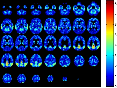
Figure 1 shows the brain image It with the value of the t-test statistic in each voxel. In this example, normals and AD images were considered in the calculation of the image It.
Figure 1.
t-test value calculated in each voxel. Regions with larger value of the t-statistic are selected to perform classification.
Student’s t-test gives us information about voxel class separability. We select those voxels i which present a t-statistic greater than a given threshold ε
| (4) |
Then, those selected voxels will be modeled using factor analysis.
Feature extraction: Factor analysis
Factor analysis is a statistical method used to describe variability among observed variables in terms of fewer unobserved variables called factors. The observed variables are modeled as linear combinations of the factors plus error. We use factor analysis to reduce the feature dimension. Factor analysis estimates how much of the variability in the data is due to common factors.
Suppose we have a set of N observable random variables, x1,…,xN with means μ1,…,μN.
Suppose for some unknown constants λij and m unobserved random variables Fj, where i∊1,…,N and j∊1,…,m, where m<N, we have
| (5) |
where zi is independently distributed error terms with zero mean and finite variance different for each observable variable. The previous expression can be also written in matrix form
| (6) |
where x is a vector of observed variables, μ is a constant vector of means, Λ is a constant N-by-m matrix of factor loadings, F is a matrix of independent, standardized common factors, and z is a vector of independently distributed error terms.
The following assumptions are imposed to the unobserved random matrix F: F and z are independent, the mean of F is equal to 0, and the covariance of F is the identity matrix. These assumptions allow computing the factor loadings Λ using a maximum likelihood approach.28 Once the factor loadings have been estimated, we rotate them using a Varimax approach which is a change of coordinates that maximizes the sum of the variance of the squared loadings. This method attempts to maximize the variance on the new axes. Thus, we obtain a pattern of loadings on each factor that is as diverse as possible. These factor loadings will be used as features for classification purposes.
There are some known regions in AD and MCI brain PET image which present hypoperfusion [lower-intensity values than for a given normal controls (NC) image]. This fact have been taken into account, preselecting those voxels in the images which present greater difference between NC, MCI, or AD images, measuring this difference using the t-test. By calculating the factor loadings considering only these preselected regions of the brain, we are not modeling the whole brain using factors but some specific regions of the images.
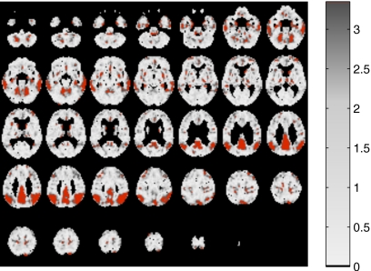
Thus, the vector of observed random variables x in the factor analysis model considered consists of a p-component vector of observations with the highest values of the t-test statistic measured in each voxel and intensity values greater than 0.35 for each PET brain image. In order to clarify what factors do actually model, in Fig. 2, we highlight selected voxels when p=2000 and normal controls and Alzheimer’s patients are considered. Therefore, in that case, x would consist of p=2000 intensity values.
Figure 2.
Solid color: p=2000 selected voxels when normal controls and AD patients are considered.
An interpretation of the meaning of the factor loadings and why they are useful to perform classification in brain image classification arises from Eq. 6. Each intensity value of the selected voxels after zero-mean normalization is expressed using a new basis using the factors F. These factors, which are estimated via factor analysis, are common to all the images. Factor loadings Λ are the weights which are also calculated using factor analysis and they are different for each image. When images of different classes are expressed using the basis given by factors F, they roughly present similar intraclass and different interclass values of factor loadings Λ. We take advantage of this behavior and use factor loadings as features for classification purposes.
Classification
The goal of the classification task is to separate a set of binary labeled training data consisting of, in the general case, p-dimensional patterns vi and class labels yi
| (7) |
so that a classifier is produced, which maps an object vi to its classification label yi. This classifier will be able to classify new examples v.
There are several different procedures to build the classification rule. We utilize the following classifiers in this work.29, 30
Multivariate normal model: Quadratic discriminant function
We suppose that v denotes a p-component random vector of observations made on any individual; v0 denotes a particular observed value of v and π1 and π2 denote the two populations involved in the problem. The basic assumption is that v has different probability distributions in π1 and π2. Let the probability density of v be f1(v) in π1 and f2(v) in π2. The simplest intuitive argument, termed the likelihood ratio rule, classifies v0 as π1 whenever it has greater probability of coming from π1 than from π2. This classification rule can be written as
| (8) |
| (9) |
The most general form of the model is to assume that πi is a multivariate normal population with mean μi and dispersion matrix Σi for i=1,2. Thus , so that we obtain
| (10) |
Hence, on taking logarithms in Eq. 8, we find that the classification rule for this model is: Allocate v0 to π1 if Q(v0)>0 and otherwise to π2, where Q(v) is the discriminant function
| (11) |
Since the terms in Q(v) include the quadratic form , which will be a function of the squares of elements of v and cross products between pairs of them, this discriminant function is known as the quadratic discriminant.
In any practical application, the parameters μ1, μ2, Σ1, and Σ2 are not known. Given two training sets, from π1 and from π2, we can estimate these parameters using the sample mean and sample standard deviation.
Multivariate normal model: Linear discriminant function
The presence of two different population dispersion matrices renders difficult the testing of hypothesis about the population mean vectors; therefore, the assumption Σ1=Σ2=Σ is a reasonable one in many practical situations. The practical benefits of making this assumption are that the discriminant function and allocation rule simplifies. If Σ1=Σ2=Σ, then
| (12) |
and the classification rule reduces to allocate v to π1 if L(v)>0 and otherwise to π2, where . No quadratic terms now exist in the discriminant function L(v), which is therefore called the linear discriminant function.
In that case, contrary to the quadratic case, we estimate the pooled covariance matrix
| (13) |
| (14) |
Support vector machines with linear kernels
Support vector machines (SVMs) have recently been proposed for pattern recognition in a wide range of applications by its ability for learning from experimental data. SVMs separate a given set of binary labeled training data with a hyperplane that is maximally distant from the two classes (known as the maximal margin hyperplane). Linear discriminant functions define decision hypersurfaces or hyperplanes in a multidimensional feature space
| (15) |
where w is the weight vector and w0 is the threshold. w is orthogonal to the decision hyperplane. The goal is to find the unknown weight vector w which defines the decision hyperplane.30
Let vi, i=1,2,…,l be the feature vectors of the training set. These belong to two different classes, π1 or π2, which for convenience in the mathematical calculations will be denoted as +1 and −1. If the classes are linearly separable, the objective is to design a hyperplane that classifies correctly all the training vectors. This hyperplane is not unique and it can be estimated maximizing the performance of the classifier, that is, the ability of the classifier to operate satisfactorily with new data. The maximal margin of separation between both classes is a useful design criterion. Since the distance from a point v to the hyperplane is given by z=|g(v)|∕∥w∥, the optimization problem can be reduced to the maximization of the margin 2∕∥w∥, with constraints by scaling w and w0 so that the value of g(v) is +1 for the nearest point in π1 and −1 for the nearest point in π2. The constraints are the following:
| (16) |
| (17) |
or, equivalently, minimizing the cost function J(w)=1∕2∥w∥2 subject to
| (18) |
RESULTS
The performance of the classification is tested on a set of 210 18F-FDG PET images (52 normals, 114 MCI, and 53 AD) using the leave-one-out method: The classifier is trained with all but one image of the database and the remaining image, which is not used to define the classifier, is then categorized. In that way, all 18F-FDG PET images are classified and the success rate is computed from the number of correctly classified subjects. This cross-validation strategy has been previously used to assess the discriminative accuracy of different multivariate analysis methods applied to the early diagnosis of Alzheimer’s disease,26 discrimination of frontotemporal dementia from AD,13 and in classifying atrophy patterns based on magnetic resonance imaging images.31
Initially, threshold ε was set to 2000 voxels. Classification schemes used in this work are binary approaches; therefore, they are able to perform classification based on a training set of two previously labeled items. Nevertheless, we work with three classes of 18F-FDG PET images, NC, MCI, and AD. Thus, we perform three different classification tasks. First, we consider only NC and AD images; second, NC versus MCI; and lastly we perform classification of NC subjects versus MCI-AD. The proposed methodology is compared to the voxel-as-features (VAF) approach with linear support vector machine classifier.32, 33, 34
NC versus AD
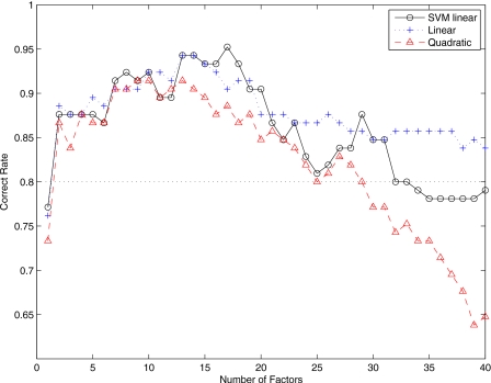
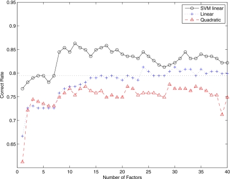
Figure 3 shows the correct rate versus the dimension m of factors F (number of unobserved random variables F). Linear classifiers perform better than the multivariate normal model with quadratic discriminant function. In general, the accuracy rate increases concomitantly with the dimension of factors for small values of m. Best correct rates are achieved when m is in the range 13–20 when we use SVM with linear kernel and multivariate normal model with linear discriminant function. Specifically, a correct rate up to 95% is reached when m=17 for SVM with linear kernels. For m>20, performance of the classification task decreases with the dimension of the number of factors.
Figure 3.
Correct rate versus number of factors when NC and AD images are considered. The dotted line is the accuracy rate obtained using voxel-as-features.
The ADNI database excludes advanced AD affected subjects. The ADNI database represents some ideal laboratory conditions, as subjects are recruited following a restricted clinical criteria to select only early AD related issues. Therefore, these favorable conditions allows proving the discrimination ability of the classifier in the discrimination of the Alzheimer’s disease in an early stage of the disease.
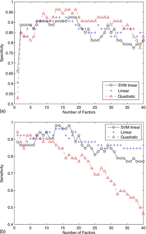
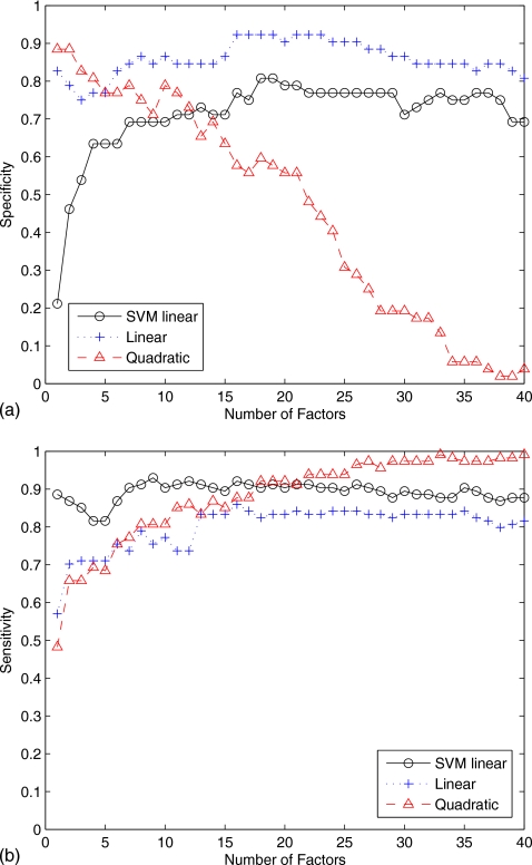
Figure 4 shows the specificity and the sensitivity versus the number of factors for the three classifiers used in this work. The quadratic discriminant function reaches higher specificity values but very low sensitivity for a number of factors greater than 10. Specificity and sensitivity results obtained using the multivariate normal model with linear discriminant function and linear SVM are roughly the same except for number of factors greater than 30, where the linear discriminant function performs slightly better.
Figure 4.
(a) Specificity versus number of factors. (b) Sensitivity versus number of factors.
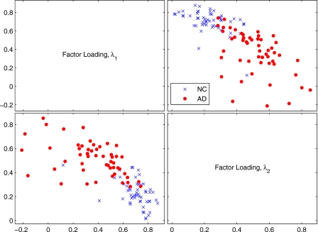
We have also drawn a scatter plot with samples from the loading factors when m=2 in Fig. 5. Figure 5 shows that even in the case in which two factor loadings are considered, most of the λ values for NC and AD images are clearly separated.
Figure 5.
Matrix of scatter plots for λ1 and λ2 when m=2.
NC versus MCI
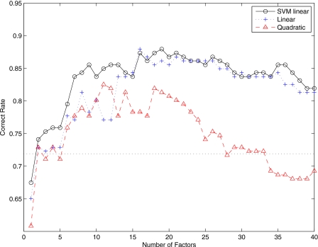
Figure 6 shows the correct rate versus number of factor loadings F when NC and MCI patients are considered. Our method presents, in that case, lower performance than when the NC and AD images were considered. This is due to the fact that images labeled as MCI present subjects with very different intensity patterns: Patients with memory complaint verified by a study partner, subjects presenting abnormal memory function, frontotemporal dementia, possibly MCI to AD converters, and subjects with general cognition and functional performance sufficiently preserved such that a diagnosis of Alzheimer’s disease cannot be made at the time of the screening visit. This wide variability in the MCI group makes the automatic computer-aided diagnosis method presented in this paper to work slightly worse than when only NC and AD subjects were considered. Equally to the NC-AD case, the quadratic classifier performs worse than the linear ones. Furthermore, from F=1 to F=14, support vector machines with linear kernels performs better than the multivariate normal model with linear discriminant function, while for F>16 they perform similarly. Our method presents better performance when the number of factor loadings is greater than 16. Specifically, the accuracy rate is greater than 85% and up to 88%.
Figure 6.
Correct rate versus number of factors when NC and MCI subjects are considered. The dotted line is the accuracy rate obtained using VAF.
Figure 7 shows the specificity and the sensitivity versus the number of factors. Let us note that the number of NC and MCI images are 52 and 114, respectively. In that case, the use of imbalanced training data set causes a possible poor performance of specificity or sensitivity since they are sample prevalence dependent. Quadratic discriminant function performs very bad in that case, reaching very high specificity values and very low sensitivity for a small number of factors. On the other hand, when the number of factors is greater than 35, quadratic discriminant function is not suitable for classification purposes since one obtains a sensitivity nearly 1 and a very low specificity. In that case, SVM linear and linear discriminant functions perform much better. Figure 7a shows that the linear discriminant function presents higher and more stable specificity values (∼0.9) for a wide range of number of factors. Figure 7b shows a similar behavior for SVM linear when sensitivity is considered: High and very stable values (∼0.9) for a wide range of number of factors.
Figure 7.
(a) Specificity versus number of factors. (b) Sensitivity versus number of factors.
NC versus MCI,AD
The number of NC and {MCI,DTA} images are 52 and 167, respectively; therefore, in that case, is inappropriate to calculate specificity or sensitivity values. A low specificity value in this largely unbalanced data set may not reflect a high false negative rate. Figure 8 depicts the accuracy rate versus the number of factors when NC subjects and a group composed of MCI and AD images are considered. In that case, SVM performs clearly better than the multivariate normal classifier with linear and quadratic discriminant function. Let note that this scenario is more difficult than classifying NC versus MCI or NC versus AD. In Sec. 3D, the diversity of MCI subjects was pointed out. In that case, a new source of heterogeneity is included in the problem and this causes the accuracy rate to be slightly lower than when only NC and MCI were considered. Despite that, the proposed methodology reaches a correct rate greater than 85% when the number of factor loadings F ranges from 8 to 19. In that case, our method also outperforms the VAF approach when using SVM.
Figure 8.
Correct rate versus number of factors when NC and MCI,AD subjects are considered. The dotted line is the accuracy rate obtained using VAF.
Performance for different threshold values ε
Up to now, threshold ε has been set to 2000 voxels. Simulations were also performed selecting 3000, 4000, and 5000 voxels (results not shown). In that case, the classification performance was slightly lower than when 2000 voxels were considered. Nevertheless, the computation time increases and the factor analysis algorithm is not able to reach convergence for large values of the number of factors. Therefore, either the relative convergence tolerance for varimax rotation (1.510−8) needs to be reduced or the iteration limit (250 iterations) increased, leading to lower computational performance.
We also compare the performance of the method using different threshold values ε (ε=2000,1500,1000,500). Table 1 presents the mean correct rate and standard deviation when the number of factors is in the interval m=[10,20]. Best results are obtained when ε=2000. Nevertheless, very good performance of the proposed methodology is reached for each one of the threshold values considered.
Table 1.
Comparison of the mean accuracy rate for m=10 to m=20 number of factor loadings for different threshold values ε. Standard deviations in parentheses.
| ε=2000 | ε=1500 | ε=1000 | ε=500 | ||
|---|---|---|---|---|---|
| NC versus AD | SVM | 0.92 (0.02) | 0.90 (0.02) | 0.87 (0.02) | 0.86 (0.02) |
| Linear | 0.92 (0.01) | 0.89 (0.01) | 0.87 (0.01) | 0.85 (0.01) | |
| Quadratic | 0.89 (0.01) | 0.85 (0.01) | 0.87 (0.01) | 0.80 (0.02) | |
| NC versus MCI | SVM | 0.86 (0.01) | 0.86 (0.02) | 0.85 (0.03) | 0.82 (0.02) |
| Linear | 0.83 (0.03) | 0.83 (0.02) | 0.82 (0.03) | 0.80 (0.01) | |
| Quadratic | 0.80 (0.02) | 0.78 (0.03) | 0.77 (0.02) | 0.80 (0.02) | |
| NC versus MCI,AD | SVM | 0.85 (0.01) | 0.84 (0.01) | 0.83 (0.02) | 0.82 (0.01) |
| Linear | 0.79 (0.01) | 0.77 (0.01) | 0.77 (0.01) | 0.75 (0.01) | |
| Quadratic | 0.76 (0.01) | 0.76 (0.01) | 0.76 (0.01) | 0.76 (0.01) |
DISCUSSION
Multinormal models with linear or quadratic discriminant functions exhibit a strong dependence on outliers as they consider that the distribution of feature vector for populations π1 and π2 follow a Gaussian distribution. Thus, this assumption could lead to poor results in the case in which the Gaussian assumption does not hold, as for instance, due to the presence of outliers in the populations. This is a typical problem which arises when the number of samples is small. Results in this work showed better performance when using SVM with linear kernel than in the case in which linear and quadratic discriminant functions were used. Specifically, in the case in which normal controls versus AD and MCI patients were considered, linear and quadratic discriminant functions obtained very poor performance. This could be due to the fact that including MCI and AD in the same group increases the heterogeneity of the feature vector and, therefore, the Gaussian assumption is not valid in that case. For this reason, and based on the results shown in the Sec. 3, support vector machine with linear kernel is the preferred of the classifiers used in this work.
In order to discuss the behavior of multinormal models for classification and the performance of this classification methods for different number of samples, simulations have been repeated using a k-fold cross-validation scheme with k=2. Specifically, when k=2, N∕2 images are used as training sets and the remaining N∕2 images are considered test images. This allows checking the performance of the classification methods when a smaller number of images is considered, and therefore, it allows us to investigate the small size sample problem empirically. In Table 2, the mean accuracy rate for m=10 to m=20 number of factor loadings obtained using leave-one-out and k-fold with k=2 are compared. The table shows that the best performance is obtained when leave-one-out is used as validation method which is an expected result. Nevertheless, let us note that good performance is also obtained when only half of the available images are used to train the classifier.
Table 2.
Comparison of the mean accuracy rate for m=10 to m=20 number of factor loadings using leave-one-out and k-fold with k=2.
| Leave-one-out | Twofold | ||
|---|---|---|---|
| NC versus AD | SVM | 0.92 | 0.87 |
| Linear | 0.92 | 0.89 | |
| Quadratic | 0.89 | 0.85 | |
| NC versus MCI | SVM | 0.86 | 0.83 |
| Linear | 0.83 | 0.81 | |
| Quadratic | 0.80 | 0.77 | |
| NC versus MCI,AD | SVM | 0.85 | 0.82 |
| Linear | 0.79 | 0.77 | |
| Quadratic | 0.76 | 0.76 |
In this work, we do not propose an analytical procedure to estimate the value of the number of factor loadings. Nevertheless, some order selection technique could be possibly used to select the number of factor loadings. We estimate the performance of the classification task for a different number of λ. This procedure allows to easily estimate an “optimal” value of the threshold in the sense that it lets us select those values of the number of factor loadings which better discriminate between populations. Thus, the plot of the accuracy rate versus the threshold enables to visually select an useful value (or a range of values) of λ for classification.
Overfitting generally occurs when a model is excessively complex, such as having too many degrees of freedom, in relation to the amount of data available. In our case, this is a possible scenario when using support vector machines with nonlinear kernels or nonlinear discriminant functions to perform classification. For this reason, we only use SVM with linear kernel. Therefore, choosing linear classifiers, or in that case, SVM with linear kernel, is supported not only by the good performance results but also by the fact that this choice lets us to avoid possible overfitting.
In addition, we would like to point out that choosing a wide range of λ values and calculating the performance of the classification task is enough for our practical purposes for different reasons. On the one hand, the estimation of a very precise and specific number of factors m is not critical as the accuracy of the proposed methodology is high for a wide range of m values for the data set studied (as instance, from m=2 to m=20 when NC versus AD was considered, and m>7 and m>8 when NC versus MCI and NC versus MCI,AD). On the other hand, if we choose to estimate the threshold value using an analytical procedure, lastly, the performance of this analytical selection procedure based on a statistical criterion should be checked in terms of accuracy, specificity, and sensitivity for different values of the number of factor loadings in order to prove the validity of the method used to estimate the order model. And, actually, this is the experimental method we use in that work to estimate useful values of the number of factors. Furthermore, the estimation of the number of λ, equal to the training procedure, only needs to be performed once as a “batch” process.
In Ref. 35, a CAD system for an automatic evaluation of the neuroimages is presented. In that work, principal component analysis (PCA) based methods are proposed as feature extraction techniques, enhanced by other linear approaches such as linear discriminant analysis or the measure of the Fisher discriminant ratio for feature selection. These features allow surmounting the so-called small sample size problem. We have used the PCA-based feature extraction method presented there as the input vector of a SVM classifier with linear kernel in order to compare to our proposed methodology. For the data set used in this work, best values of the correct rate, specificity, and sensitivity using both approaches are shown in Table 3.
Table 3.
Comparison between the performance of the FA proposed in this work and the PCA-based method (PCA) in Ref. 35. m is the number of factors or components.
| FA | PCA | ||
|---|---|---|---|
| NC versus AD | Acc | 95.2 | 89.5 |
| Sen | 98.1 | 84.5 | |
| Spe | 92.5 | 84.7 | |
| m | 17 | 8 | |
| NC versus MCI | Acc | 88.0 | 81.3 |
| Sen | 91.2 | 97.4 | |
| Spe | 80.8 | 46.1 | |
| m | 19 | 30 | |
| NC versus MCI,AD | Acc | 86.3 | 82.2 |
| Sen | 92.8 | 92.21 | |
| Spe | 65.4 | 50 | |
| m | 11 | 30 |
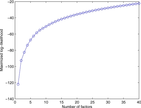
Despite of the fact that an empirical estimation of m is enough for our purposes, we suggest a possible method to calculate an optimal m value using an analytical procedure studying the value of the log-likelihood. Figure 9 plots the log-likelihood versus m (the number of factors) in the case in which NC versus MCI,AD images are considered. It can be seen how increasing m also increases the ability of the factor loadings to model the data more accurately (the log-likelihood increases). Log-likelihood values when m is small (from m=1 to m=7) present a great variability. This coincides with the same range of values in which our algorithm does not provide high correct rate, possibly due to the fact that the number of factors is not enough to model correctly the variability of the data.
Figure 9.
Log-likelihood versus the number of factors m in the case in which images NC versus MCI,AD are considered.
The factor analysis model in Eq. 6 can also be specified as
| (19) |
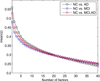
where cov(z) is a p-by-p diagonal matrix of specific variances and p is the number of observed variables. Finally, we study the values of cov(z) representing the mean of the diagonal values of matrix cov(z) for each group NC versus AD, NC versus MCI, and NC versus MCI,AD in Fig. 10. In these three cases the values are very similar and, as it was expected, they decrease as the number of factors increase, because for greater values of m, the factors are more capable to model the observed random variables.
Figure 10.
Mean of diagonal values in matrix cov(z) versus number of iterations. Circles: NC,AD. Squares: NC,MCI. Triangles: NC,MCI,AD.
CONCLUSIONS
In this work, an automatic procedure to assist the diagnosis of early Alzheimer’s disease is presented. The proposed methodology is based on the selection of voxels of interest using the t-test and a posterior reduction of the feature dimension using factor analysis. Factor loadings were used as features of three different classifiers: Two multivariate Gaussian mixture models, with linear and quadratic discriminant function, and a support vector machine with linear kernel which was found to achieve the highest accuracy rate. The best results were obtained when normal and Alzheimer’s disease subjects were considered. Specifically, an accuracy rate greater than 90% were obtained in that case for a wide range of number of factors. Furthermore, results were compared to the voxel-as-features and a PCA-based approach. The proposed methodology was found to perform clearly better.
ACKNOWLEDGMENTS
This work was partly supported by the Spanish Government under the PETRI DENCLASES (Grant No. PET2006-0253), Grant No. TEC2008-02113, NAPOLEON (Grant No. TEC2007-68030-C02-01) projects, and the Consejería de Innovación, Ciencia y Empresa (Junta de Andalucía, Spain) under the Excellence Projects TIC-02566 and TIC-4530. Data collection and sharing for this project was funded by the ADNI (National Institutes of Health Grant No. U01 AG024904). ADNI is funded by the National Institute on Aging, the National Institute of Biomedical Imaging and Bioengineering, and through generous contributions from the following: Abbott, AstraZeneca AB, Bayer Schering Pharma AG, Bristol-Myers Squibb, Eisai Global Clinical Development, Elan Corporation, Genentech, GE Healthcare, GlaxoSmithKline, Innogenetics, Johnson and Johnson, Eli Lilly and Co., Medpace, Inc., Merck and Co., Inc., Novartis AG, Pfizer Inc., F. Hoffman-La Roche, Schering-Plough, Synarc, Inc., and Wyeth, as well as nonprofit partners the Alzheimer Association and Alzheimer Drug Discovery Foundation, with participation from the U.S. Food and Drug Administration. Private sector contributions to ADNI are facilitated by the Foundation for the National Institutes of Health (www.fnih.org). The grantee organization is the Northern California Institute for Research and Education and the study is coordinated by the Alzheimer’s Disease Cooperative Study at the University of California, San Diego. ADNI data are disseminated by the Laboratory for Neuro Imaging at the University of California, Los Angeles. This research was also supported by NIH Grant Nos. P30 AG010129 and K01 AG030514 and the Dana Foundation.
References
- Brookmeyer R., Gray S., and Kawas C., “Projections of Alzheimer’s disease in the United States and the public health impact of delaying disease onset,” JAMA, J. Am. Med. Assoc. 88, 1337–1342 (1998). [DOI] [PMC free article] [PubMed] [Google Scholar]
- Brookmeyer R., Johnson E., Ziegler-Graham K., and Arrighi M., “Forecasting the global burden of Alzheimer’s disease,” Alzheimer's & Dementia 3, 186–191 (2007). 10.1016/j.jalz.2007.04.381 [DOI] [PubMed] [Google Scholar]
- Johnson E., Brookmeyer R., and Ziegler-Graham K., “Modeling the effect of Alzheimer’s disease on mortality,” The International Journal of Biostatistics 3(1), Article 13 (2007). 10.2202/1557-4679.1083 [DOI] [PubMed]
- Alexander G. E., Pietrini P., Rapoport S. I., and Reiman E. M., “Longitudinal PET evaluation of cerebral metabolic decline in dementia: A potential outcome measure in Alzheimer’s disease treatment studies,” Am. J. Psychiatry 159, 738–745 (2002). 10.1176/appi.ajp.159.5.738 [DOI] [PubMed] [Google Scholar]
- Langbaum J. B., Vhen K., Lee W., Reschke C., Bandy D., Fleisher A. S., Alexander G. E., Foster N. L., Weiner M. W., Koeppe R. A., Jagust W. J., and Reiman E. M., “Categorical and correlation analyses of baseline fluorodeoxyglucose positron emission tomography images from the Alzheimer’s Disease Neuroimaging Initiative (ADNI),” Neuroimage 45, 1107–1116 (2009). 10.1016/j.neuroimage.2008.12.072 [DOI] [PMC free article] [PubMed] [Google Scholar]
- Minoshima S., Goirdani B., Berent S., Frey K. A., Foster N. L., and Khul D. E., “Metabolic reduction in the posterior cingulate cortex in very early Alzheimer’s disease,” Ann. Neurol. 42, 85–94 (1997). 10.1002/ana.410420114 [DOI] [PubMed] [Google Scholar]
- Mosconi L. et al. , “Multicenter standardized 18F-FDG PET diagnosis of mild cognitive impairment, Alzheimer’s disease and other dementias,” J. Nucl. Med. 49, 390–398 (2008). 10.2967/jnumed.107.045385 [DOI] [PMC free article] [PubMed] [Google Scholar]
- Silverman D. H., Small G. W., and Chang C. Y., “Positron emission tomography in evaluation of dementia: Regional brain metabolism and long-term outcome,” JAMA, J. Am. Med. Assoc. 286, 2120–2127 (2001). 10.1001/jama.286.17.2120 [DOI] [PubMed] [Google Scholar]
- Braak H. and Braak E., “Diagnostic criteria for neuropathologic assessment of Alzheimer’s disease,” Neurobiol. Aging 18, S85–S88 (1997). 10.1016/S0197-4580(97)00062-6 [DOI] [PubMed] [Google Scholar]
- Cummings J. L., Vinters H. V., Cole G. M., and Khachaturian Z. S., “Alzheimer’s disease: Etiologies, pathophysiology, cognitive reserve, and treatment opportunities,” Neurology 51, S2–S17 (1998). [DOI] [PubMed] [Google Scholar]
- Hoffman J. M., Welsh-Bohmer K. A., and Hanson M., “FDG PET imaging in patients with pathologically verified dementia,” J. Nucl. Med. 41, 1920–1928 (2000). [PubMed] [Google Scholar]
- Ng S., Villemagne V. L., Berlangieri S., Lee S. -T., Cherk M., Gong S. J., Ackermann U., Saunder T., Tochon-Danguy H., Jones G., Smith C., O’Keefe G., Masters C. L., and Rowe C. C., “Visual assessment versus quantitative assessment of 11C-PIB PET and 18F-FDG PET for detection of Alzheimer’s disease,” J. Nucl. Med. 48, 547–552 (2007). 10.2967/jnumed.106.037762 [DOI] [PubMed] [Google Scholar]
- Higdon R., Foster N. L., Koeppe R. A., DeCarli C. S., Jagust W. J., Clark C. M., Barbas N. R., Arnold S. E., Turner R. S., Heidebrink J. L., and Minoshima S., “A comparison of classification methods for differentiating fronto-temporal dementia from Alzheimer’s disease using FDG-PET imaging,” Stat. Med. 23, 315–326 (2004). 10.1002/sim.1719 [DOI] [PubMed] [Google Scholar]
- Duin R. P. W., “Classifiers in almost empty spaces,” in Proceedings of the 15th International Conference on Pattern Recognition (IEEE, Barcelona, 2000), Vol. 2, pp. 1–7.
- Folstein M., Folstein S. E., and McHugh P. R., “‘Mini-mental state’: A practical method for grading the cognitive state of patients for the clinician,” J. Psychiatr. Res. 12, 189–198 (1975). 10.1016/0022-3956(75)90026-6 [DOI] [PubMed] [Google Scholar]
- Morris J. C., “Clinical dementia rating,” Neurology 43, 2412–2414 (1993). [DOI] [PubMed] [Google Scholar]
- Spreen O. and Strauss E., A Compendium of Neuropsychological Tests: Administration, Norms, and Commentary, 2nd ed. (Oxford University Press, New York, 1998). [Google Scholar]
- Blacker D., Albert M. S., Bassett S. S., Go R. C., Harrell L. E., and Folstein M. F., “Reliability and validity of NINCDS-ADRDA criteria for Alzheimer’s disease. The National Institute of Mental Health Genetics Initiative,” Arch. Neurol. 51, 1198–1204 (1984). [DOI] [PubMed] [Google Scholar]
- Loewenstein D. A., Ownby R. M. D., Schram L., Acevedo A., Rubert M., and Argelles T., “An evaluation of the NINCDS-ADRDA neuropsychological criteria for the assessment of Alzheimer’s disease: A confirmatory factor analysis of single versus multi-factor models,” J. Clin. Exp. Neuropsychol 23, 274–284 (2001). 10.1076/jcen.23.3.274.1191 [DOI] [PubMed] [Google Scholar]
- McKhann G., Drachman D., Folstein M., Katzman R., Price D., and Stadlan E. M., “Clinical diagnosis of Alzheimer’s disease: Report of the NINCDS-ADRDA work group under the auspices of Department of Health and Human Services Task Force on Alzheimer’s disease,” Neurology 34, 939–944 (1984). [DOI] [PubMed] [Google Scholar]
- Salas-Gonzalez D., Górriz J. M., Ramírez J., Lassl A., and Puntonet C. G., “Improved Gauss-Newton optimization methods in affine registration of SPECT brain images,” Electron. Lett. 44, 1291–1292 (2008). 10.1049/el:20081838 [DOI] [Google Scholar]
- Woods R. P., Grafton S. T., Holmes C. J., Cherry S. R., and Mazziotta J. C., “Automated image registration: I. General methods and intrasubject, intramodality validation,” J. Comput. Assist. Tomogr. 22, 139–152 (1998). 10.1097/00004728-199801000-00027 [DOI] [PubMed] [Google Scholar]
- Ashburner J. and Friston K. J., “Nonlinear spatial normalization using basis functions,” Hum. Brain Mapp 7, 254–266 (1999). [DOI] [PMC free article] [PubMed] [Google Scholar]
- Chaves R., Ramírez J., Górriz J. M., López M., Salas-Gonzalez D., Álvarez I., and Segovia F., “SVM-based computer-aided diagnosis of the Alzheimer’s disease using t-test NMSE feature selection with feature correlation weighting,” Neurosci. Lett. 461, 293–297 (2009). 10.1016/j.neulet.2009.06.052 [DOI] [PubMed] [Google Scholar]
- Górriz J. M., Lassl A., Ramírez J., Salas-Gonzalez D., Puntonet C. G., and Lang E. W., “Automatic selection of ROIs in functional imaging using Gaussian mixture models,” Neurosci. Lett. 460, 108–111 (2009). 10.1016/j.neulet.2009.05.039 [DOI] [PubMed] [Google Scholar]
- Ramírez J., Górriz J. M., Salas-Gonzalez D., Romero A., López M., Alvarez I., and Gómez-Río M., “Computer aided diagnosis of Alzheimer's type dementia combining support vector machines and discriminant set of features,” Information Sciences (in press).
- Salas-Gonzalez D., Górriz J. M., Ramírez J., López M., Álvarez I., Segovia F., Chaves R., and Puntonet C. G., “Computer aided diagnosis of Alzheimer’s disease using support vector machines and classification trees,” Phys. Med. Biol. 55, 2807–2817 (2010). 10.1088/0031-9155/55/10/002 [DOI] [PubMed] [Google Scholar]
- Harman H. H., Modern Factor Analysis (University of Chicago Press, Chicago, 1976). [Google Scholar]
- Principles of Multivariate Analysis: A User’s Perspective, edited by Krzanowski W. J. (Oxford University Press, New York, 1988). [Google Scholar]
- Vapnik V. N., Statistical Learning Theory (Wiley, New York, 1998). [Google Scholar]
- Fan Y., Batmanghelich N., Clark C. M., Davatzikos C., and the Alzheimer's Disease Neuroimaging Initiative, “Spatial patterns of brain atrophy in MCI patients, identified via high-dimensional pattern classification, predict subsequent cognitive decline,” Neuroimage 39(4), 1731–1743 (2008). 10.1016/j.neuroimage.2007.10.031 [DOI] [PMC free article] [PubMed] [Google Scholar]
- Fung G. and Stoeckel J., “SVM feature selection for classification of SPECT images of Alzheimer’s disease using spatial information,” Knowledge Inf. Syst. 11, 243–258 (2007). 10.1007/s10115-006-0043-5 [DOI] [Google Scholar]
- Stoeckel J., Ayache N., Malandain G., Koulibaly P. M., Ebmeier K. P., and Darcourt J., “Automatic classification of SPECT images of Alzheimer’s disease patients and control subjects,” in Medical Image Computing and Computer-Assisted Intervention—MICCAI 2004, edited by Barillot C., Haynor D. R., and Hellier P. (Springer, Berlin/Heidelberg, 2004) [Google Scholar]; [Lect. Notes Comput. Sci. 3217, 654–662 (2004). 10.1007/978-3-540-30136-3_80 [DOI] [Google Scholar]
- Stoeckel J., Malandain G., Migneco O., Koulibaly P. M., Robert P., Ayache N., and Darcourt J., “Classification of SPECT images of normal subjects versus images of Alzheimer’s disease patients,” in Medical Image Computing and Computer-Assisted Intervention Conference—MICCAI 2001, edited by Niessen W. and Viergever M. (Springer, Berlin/Heidelberg, 2001) [Google Scholar]; Stoeckel J., Malandain G., Migneco O., Koulibaly P. M., Robert P., Ayache N., and Darcourt J.,[ Lect. Notes Comput. Sci. 2208, 666–674 (2001). 10.1007/3-540-45468-3_80 [DOI] [Google Scholar]
- López M., Ramírez J., Górriz J. M., Salas-Gonzalez D., Álvarez I., Segovia F., and Puntonet C. G., “Automatic tool for the Alzheimer’s disease diagnosis using PCA and Bayesian classification rules,” Electron. Lett. 45, 389–391 (2009). 10.1049/el.2009.0176 [DOI] [Google Scholar]


