Modified least-variant set normalization for miRNA microarray

Abstract

MicroRNAs (miRNAs) are short noncoding RNAs that are involved in post-transcriptional regulation of mRNAs. Microarrays have been employed to measure global miRNA expressions; however, because the number of miRNAs is much smaller than the number of mRNAs, it is not clear whether traditional normalization methods developed for mRNA arrays are suitable for miRNA. This is an important question, since normalization affects downstream analyses of the data. In this paper we develop a least-variant set (LVS) normalization method, which was previously shown to outperform other methods in mRNA analysis when standard assumptions are violated. The selection of the LVS miRNAs is based on a robust linear model fit of the probe-level data that takes into account the considerable differences in variances between probes. In a spike-in study, we show that the LVS has similar operating characteristics, in terms of sensitivity and specificity, compared with the ideal normalization, and it is better than no normalization, 75th percentile-shift, quantile, global median, VSN, and lowess normalization methods. We evaluate four expression-summary measures using a tissue data set; summarization from the robust model performs as well as the others. Finally, comparisons using expression data from two dissimilar tissues and two similar ones show that LVS normalization has better operating characteristics than other normalizations.

INTRODUCTION

MicroRNAs are short ∼18–24-nucleotide (nt)-long noncoding RNAs that down-regulate mRNA expression by binding to the 3′ untranslated region of their target mRNAs. They have recently been found to play a significant role in human cancer (Pasquinelli et al. 2005; Fabbri et al. 2008; Guarnieri and DiLeone 2008). The miRbase release 14.0 reports 721 human miRNAs, each of which can potentially regulate many target genes (Griffiths-Jones 2004; Griffiths-Jones et al. 2006, 2008; Betel et al. 2008).

Microarray technology is a commonly used method to measure the expression of hundreds of miRNAs simultaneously, but there are still problems in the preprocessing of the data. Apart from the true signal, microarray data show systematic differences between samples due to technical factors. To reduce these systematic technical biases, a normalization step is needed before downstream statistical analysis. Different choices of normalization methods exist, all previously developed for mRNA arrays, but there is no consensus on their relative performance on miRNAs. These two classes of RNAs are sufficiently distinct as to raise questions whether existing normalization methods are suitable for miRNAs. Several studies comparing normalization methods for miRNA microarray do not show consistent results. Hua et al. (2008) suggest that the lowess method is the best. In contrast, Rao et al. (2008) and Zhao et al. (2010) show evidence that favors quantile-based normalization, which is among the most commonly used methods. However, quantile normalization forces each array to have the exact same empirical distribution of intensities. In practice, this strong assumption can hardly be expected to hold for miRNAs, since the number of miRNAs is small, so the profile is likely to vary across arrays. Also, unlike for mRNAs, it is not sensible to make assumptions about the nonregulation of the majority of the miRNAs. We need to develop a robust method that can perform a good normalization on arrays from differentiated cell types with a small number of available features.

Normalization methods for mRNAs rely on two standard assumptions: (1) the majority of features do not vary between samples and (2) the proportions of up- and down-regulated expressions are approximately equal. To compensate for the lack of robustness in the existing methods, the least-variant set (LVS) normalization for mRNA arrays was developed by Calza et al. (2007) based on data-driven housekeeping genes. For Affymetrix gene-expression arrays, they show that it outperforms other normalization methods when the standard assumptions are not satisfied. The total information extracted from probe-level intensity data of all samples is modeled as a function of array and probe effects. The method selects genes with the smallest array-to-array variation, called LVS genes, and uses these as the reference set for normalization.

Our adaptation for miRNAs involves a more complex model to identify the LVS. Since the selection is done using a set of parametric models, modeling is crucial for making valid inferences from the data to choose the ideal housekeeping miRNAs. Based on our empirical analyses, probes tend to show considerable differences in within-probe variances. Our approach here is to jointly model mean and dispersion, instead of assuming constant residual variation, the dispersion parameters are modeled as a function of array and probe effects (Lee et al. 2006).

The goal of this study is to develop a modified version of the LVS normalization method for miRNA arrays. The method is applicable to any platform with replicated-probe design, for example, Agilent microarray, miRCURY from Exiqon, and miRXplore from Miltenyi Biotec. In our examples, we implement the method on data sets from Agilent miRNA arrays. Hereafter we refer to default normalization as the one performed by Agilent Feature Extraction Software (v9.5). The performance of the algorithm is evaluated by computing the sensitivity and specificity in identifying differentially expressed (DE) miRNAs in a spike-in (Willenbrock et al. 2009) and a normal-tissue microarray together with an RT-PCR (Ach et al. 2008; Lee et al. 2008) data set. LVS performs similarly to the ideal normalization that is available for the spike-in data, and it is better than the default preprocessing method, the 75th percentile-shift, quantile, global median, VSN, lowess, or invariant-set (inv-P) normalization method from Pradervand (2009).

RESULTS

We first summarize the analysis steps using the LVS normalization (see Materials and Methods):

1. Fit a robust linear model (1) on the background-corrected raw probe-level data, where the mean and variance are modeled jointly.

2. Take a subset of the miRNAs that have the least variation across arrays, determined from the plot of array-effect test statistics versus residual standard deviations (SDs) from the model in Step 1.

3. Normalize the raw data at either the miRNA level or the probe level, where the miRNA level normalization requires the data to be summarized first.

Variance heterogeneity

Data are structured with every single miRNA having several probes each one with a few repetitions. The first step in LVS normalization is to fit a robust linear model (RLM) at each set of probe-level intensity data. The scatter plot of residuals versus fitted values from the linear model in Figure 1A shows very strong heterogeneous variances between probes. Figure 1B also shows the histogram of P-values from the Levene test on homogeneity of variances of probes within the same miRNA. An estimate of the proportion of true homogeneity of variances is , indicated by the dotted line. This means 57% of the miRNAs have residual variance that is probe-dependent. Failing to incorporate such mean–variance relationship in the analysis will result in inefficiency in the estimation of the array and probe effects. Thus, it may cause misleading information on array-to-array variability for some miRNAs. For the normal-tissue data set, we observe that in the joint model, more than half of the miRNAs with two or more probes have significant probe effect. Moreover, the estimates of probe and array effects are different from the ones estimated under the assumption of constant residual variance.

FIGURE 1.

(A) A residual plot for model fitted into one miRNA with approximate median value of Levene's F-value statistics. The random variations of the residuals seem to associate with the fitted values. This pattern indicates that the residual variance is not constant. (B) The distribution of P-values from the Levene test for every miRNA targeted by two or more probes in normal-tissue data. A large proportion of P-values is less than 0.05 indicating homogeneity of variances is violated for most linear models fitted.

Spike-in data

The array-to-array variability is measured by the χ² statistic (see Materials and Methods). Figure 2 shows the square-root of the χ² statistic as a function of the logarithm of the residual standard deviation from the probe-level robust linear model for spike-in miRNA data, called the “RA-plot.” This is using (1) Normexp (Irizarry et al. 2003) and (2) Edwards background correction (Edwards 2003). Crosses represent features that are not hybridized, therefore they represent only spurious signal, while triangles are spike-in miRNAs, which are spiked in at equal concentration, called fold change one (FC1) miRNAs. As expected, FC1 features have a small array-to-array variability and most of them would be selected as LVS miRNAs in both scenarios. Since the FC1 miRNAs are the ideal housekeeping miRNAs in this case, LVS successfully selects them to provide the theoretically best normalization. If we consider the effect of background correction on nonspiked features, the Normexp method seems to introduce a spurious variability as shown by the relatively high array effect on the RA-plot (Fig. 2A). On the other hand, background correction based on the Edwards method places the vast majority of the nonspiked features at the bottom, which is consistent with the fact that their variation accounts only for random noise. Thus, the RA plot is informative in telling us that the Edwards method is better than the Normexp.

FIGURE 2.

RA plots for spike-in data using Normexp background correction (A) or Edwards background correction (B). In both cases the correction is performed on foreground values after local background estimates subtraction. Points below the quantile curves are chosen as the LVS miRNAs.

We then compare the ability of expression measures to detect differential expression by evaluating gains in sensitivity and specificity after normalization. True positives are defined as miRNAs with a FC different from 1. We compare Group B with Group A using a moderated t-test (Smyth 2004). The proportion of true positive miRNAs identified is plotted against false discovery proportion. In particular, the Normexp method cannot identify all truly differentially expressed miRNAs allowing up to a 10% fraction of false positives. Moreover, the average rank of the P-values for FC1 or non-spiked-in features is higher for Edwards compared to Normexp (659 versus 574), indicating higher specificity.

We next compare the different normalization procedures (Fig. 3). First we note that for the spike-in data we can compute an ideal normalization based on the FC1 miRNAs, i.e., features that are known to be constant across the arrays. They are useful here to indicate the best possible normalization, but in practice these FC1 miRNAs are of course not available. Both LVS normalization methods using joint modeling and standard RLM achieve similar level of sensitivity and specificity compared to the FC1 normalization. This is perhaps not surprising, since the RA plots in Figure 2 show that the LVS method identifies the FC1 genes and use them as the reference set for normalization.

FIGURE 3.

Sensitivity and specificity of the normalization methods for spike-in data. Proportion of true discoveries are plotted against the proportion of false discoveries. Positives are defined as miRNAs both present and with FC not equal to 1.

LVS based on the Edwards background correction performs better than the other methods. Unnormalized values are substantially worse than the normalized values. At false discovery proportion around 2%, the true discovery proportion varies from around 50% to 90%, indicating that a proper normalization procedure matters, and in this case the LVS method works well.

Normal-tissue data

Raw data are first processed with the Edwards background correction. Using τ = 0.7, a total of 372 out of 534 miRNAs with array effects below the estimated quantile regression line are used as the LVS for normalization based on the VSN algorithm (Huber et al. 2002).

To assess the effect of summarization we compare four different algorithms: simple within-probe average, total gene signal (v9.5), and summarized array effect using median polish and RLM. Table 1 shows the correlation coefficient of microarray data versus qPCR data before and after summarization. Using a robust method, like RLM or median polish we would account for within-probe variability, thus it should provide a theoretically better summarization method than the simplest method for averaging the intensity of different probes.

TABLE 1.

Attributes of miRNAs with a different level of correlation coefficient produced by four summarization methods

The correlation between the raw miRNA data and qPCR data of 60 miRNAs is very high. Most expressed miRNAs (51/60) have a correlation coefficient larger than 0.9. The results show that our preprocessing and summarization does not deteriorate the original good correlation. In addition, we find that r² is related to the magnitude and level of expression (Table 1). For example we have r² ≥ 0.99 for probes with mean signal (on log₂ scale) above 12, and r² < 0.95 for probes with mean intensity below 11. Therefore, highly expressed miRNAs have a more consistent signal.

Figure 4 shows box plots of data distribution both with background correction only (A) and after summarization and normalization (B). Samples are grouped and plotted according to the source tissue and colored in white or gray to make the grouping obvious. Data are normalized using the LVS joint-model followed by VSN at the miRNA level, i.e., after RLM summarization. While raw data are relatively scattered, LVS normalization makes the data distribution within tissue more even, at the same time preserving some distinction between tissues to some extent. Had we applied the quantile normalization we would not have observed differences between the tissue types.

FIGURE 4.

Box plots of background corrected probe intensity for normal-tissue data before normalization and summarization on arcsinh scale (A) and after normalization and summarization using LVS on arcsinh scale (B). Different tissues are plotted in order and alternatively colored in white and gray.

Normal-tissue RT-PCR data

To evaluate the performance of the normalization methods in terms of sensitivity and specificity, we compare the expression both in two very distinct tissues, i.e., brain and heart, and in two tissues where we expect to find little differences, i.e., skeletal muscle and heart.

We take a subset from raw data of Ach et al. (2008) to get tissues of interest only, i.e., heart versus brain, and heart versus skeletal muscle. For these data, the LVS normalization using joint modeling is compared to:

1. default method (v9.5);

2. default method followed by a 75th percentile normalization (Agilent 2008);

3. quantile normalization (Wernisch et al. 2003);

4. invariant-set method (Pradervand 2009) using the code provided by the author at http://www.unil.ch/dafl/page58744.html;

5. global median normalization;

6. variance stabilizing normalization (VSN) (Huber et al. 2002);

7. locally weighted scatter plot smoothing (lowess) (Yang et al. 2002).

Differentially expressed miRNAs are defined using both qPCR-based fold changes (FCs) and P-values computed on array data. This allows us to use FC, computed by the ratio of the expression between two tissues, from qPCR data as an independent gold standard when we evaluate a set of top significant genes identified by all algorithms. Specifically, differentially expressed miRNAs are those with qPCR FC > 3, either over- or underexpression, and P-value < 0.01.

In order to increase the number of validated miRNAs, we combine qPCR values provided by Lee et al. (2008) with those produced by Ach et al. (2008). Figure 5 shows a Venn diagram profiling miRNA measured, respectively, in Lee et al.’s qPCR data, Ach et al.’s microarray, and qPCR data. Overall, 194 miRNAs comprise 174 from Lee et al. and 20 from normal tissue data. For heart and brain tissues, 71 out of 194 miRNAs have absolute FC > 3 (FC = brain/heart) and P-value < 0.01. More specifically, 41 have FC ≥ 3, 30 have FC ≤ 1/3. For skeletal muscle and heart, 25 miRNAs have absolute FC > 3 and P-value < 0.01. Namely, 11 have FC ≥ 3 and 14 have FC ≤ 1/3.

FIGURE 5.

Venn diagram for the miRNAs profiled respectively in Lee et al.’s qPCR data, Ach et al.’s microarray, and qPCR data.

Figure 6 shows the operating characteristic (OC) curves for both comparisons. Clearly, in the situation when we expect to have some differential expression (A), as between brain and heart tissues, LVS normalization performs better than all the other procedures. Normalization on the 75th percentile is the worst, followed by quantile normalization, inv-P, default signal without any normalization, lowess, global median; VSN is almost as good as LVS. The modifications of the data using 75th percentile-shift or quantile normalization methods are too severe, dramatically reducing the ability to detect the signal. Of course, in practice, we have no way of knowing that this is the case.

FIGURE 6.

Sensitivity and specificity analysis of the normalization methods both in two extremely different tissues (brain and heart) and in two similar tissues (skeletal muscle and heart). Proportion of true discoveries are plotted against the proportion of false discoveries. Positives are defined as miRNAs with a FC (FC = brain or skeletal muscle/heart) >3, either over- or underexpression. Panels (A) and (C) show OC curves for brain vs. heart comparisons for all the different methods considered. Similarly, panels (B) and (D) show OC curves for skeletal muscle vs. heart comparisons. LVS has the advantage of being flexible enough to successfully adapt to either situation.

What is also interesting is the lack of consistency in the default normalization results compared to those for the spike-in data (Fig. 3), thus indicating the lack of robustness. Table 2 shows the AUC values relative to Figure 3, as well as values for sensitivity and specificity achieved by the normalization algorithms at different numbers of top significant miRNAs considered. Again, the LVS algorithm clearly outperforms all the others in the heart versus brain comparison. For the two similar tissues the methods show less difference, though LVS still performs among the best in terms of AUC.

TABLE 2.

Sensitivity and specificity is expressed as percentage for varying number of top genes used as threshold for normal tissue data (10, 40, 70, 100, and 130 are the numbers of genes)

When we have more homogeneous samples with small fold changes, as between brain and skeletal muscle tissues, the LVS still performs better than the other procedures. However, the assumptions underlying quantile, global median, or 75th percentile normalization are more reasonable, leading to more similar performances to the LVS, although now the inv-P and lowess methods perform the worst. Both of these examples show that LVS has the advantage of being flexible enough to adapt to the underlying differential-expression pattern.

DISCUSSION

Although microarray technologies have been in use for over a decade, some technical aspects of data preprocessing, such as normalization, are still a matter of debate even in the established field of mRNA expression. A major assumption in most normalization procedures employed in mRNA preprocessing is that most genes are not differentially expressed, and that for those differentially expressed there is an approximately balanced proportion of over- and underexpression. While this is generally acceptable for mRNAs, it is unrealistic for miRNAs both biologically, as we do not expect most miRNAs to be nondifferentially expressed, and technically, as the small number of features available on miRNA array chips makes the standard normalization algorithms highly unstable (Davison et al. 2006).

Since the early days of array technologies, it has been suggested that the optimal approach for data normalization would make use of reliable control features that are consistently stable across samples and experimental conditions, and structurally similar to the targeted molecules. According to these criteria, spike-in mRNAs, synthetic miRNAs, housekeeping genes, or small noncoding RNAs (Kiss 2002) are not feasible choices.

A few recent papers (Pradervand 2009; Wang et al. 2010) explore the application of a well-known normalization procedure inherited from the mRNA field, commonly known as invariant-set normalization. The underlying idea is to select a set of reference features based on a data-driven procedure rather than from a priori biological knowledge. These reference features are identified as the most consistently expressed, based on some measure of variability across samples. We propose a modified LVS normalization procedure, for selecting miRNAs with least array-to-array variability using a joint GLM, and choosing features with potentially high information content. The information content is derived as a measure of between-sample variability computed at probe level and accounting for within-miRNA probe variation. Features with smaller variability are the best candidates for acting as reference features for between-array normalization, which can be performed either using smooth splines or VSN, a well-known algorithm for mRNA data calibration.

The proposed method is an adaptation of a similar algorithm developed for Affymetrix mRNA array (Calza et al. 2007), to a modified one for the miRNA Agilent platform, with an improved modeling of the data. The main motivation of the joint GLM modeling stands in the heterogeneous variance of intensities across probes for a large proportion of miRNAs, so that a standard RLM would not efficiently estimate array and probe effects, and thus would likely result in suboptimal identification of the reference set for normalization. Generally speaking, LVS normalization will have widespread utility in other platforms with replicated-probe design. Platform miRCURY has just a lesser numbers of probes and replicates for each miRNA, compared to Agilent on average. Instead of one-color design, miRXplore has two channels, where each miRNA is targeted by four repetitions. In such case, color effect can be included to correct for dye bias.

Commonly, microarray technologies are employed to identify a signature of differentially expressed RNAs among two or more biological conditions. In this regard, an optimal preprocessing procedure would be the one that maximizes the ability of any statistical test to identify a true signature and minimizes the burden of false discoveries. Our study has shown that, in the OC curves, the proposed LVS algorithm improves on existing normalization procedures in terms of sensitivity and specificity, especially with a relatively high number of differentially expressed features. Moreover, it is flexible enough to successfully adapt to various scenarios.

It must be noted that the spike-in miRNA data set is not the ideal setting. Although allowing us to compute true and false discoveries, the data are too clean; in this situation almost all normalization procedures perform reasonably well. A real data set is used to evaluate the consistency of the suggested summarization procedure, comparing array-based signals and qPCR data. The correlation of the summarized signal based on RLM with the qPCR gold standard is as good as the one computed by Agilent's Feature Extraction software.

The main advantage of the suggested summarization procedure is that it allows a flexible choice of the preprocessing steps, like local background correction, which in our experience might have a great impact on overall signal and requires a careful evaluation. Indeed, applying our method to the spike-in data we show how the background correction method Normexp, which performed better in a recent paper comparing several background correction methods for two-colors microarray (Ritchie, et al. 2007), is inflating the array-to-array variability for nonspiked probes, resulting in a slightly reduced performance compared to another well-known method, Edwards. Given the tiny sample size of the spike-in experiment, as well as the uniqueness of the design, we do not speculate about which background method is actually better than the other but rather stress the importance of evaluating the effect of preprocessing steps on data distribution.

The idea underlying the LVS algorithm of selecting invariant features as a reference subset for normalization originates from the usage of housekeeping genes for normalization commonly in qPCR. The usage of putative housekeeping genes for microarray normalization is deprecated, as many studies report a considerable variability under some experimental condition (Lee et al. 2002). Then again, data-driven selection procedures have been suggested and applied on mRNA platforms (Li and Wong 2001; Tseng et al. 2001), and only recently extended to the miRNA framework (Pradervand 2009; Wang et al. 2010).

The advantage of our method over other invariant-set based procedures is that, exploiting more information, it operates on the raw signal prior to any processing, such as local background correction and summarization, and without any additional external data (Wang et al 2010). The basic idea is to simply compute a measure of between-sample variability accounting for heterogeneity of between-probe variances within an miRNA, thus exploiting all information content in probe-level data. The result is a more sophisticated version of a variance filtering procedure, where low-variance features are used as a reference set for normalization. The rather straightforward method does not require any specific assumption, such as the existence of mixing distributions, so it is applicable in most of situations.

The increasing availability of genomic data targeting different molecules or detecting different types of signal like mRNA arrays, exon arrays, CGH, and miRNA arrays opens new avenues for investigation. To be able to exploit as much information as possible, a careful data preprocessing is mandatory. While a huge amount of work has been done for well-known frameworks like mRNA and CGH, only recently miRNA platforms have attracted some attention. We propose a new algorithm for the normalization of miRNA data produced by Agilent technology and evaluate its performance in terms of sensitivity and specificity for detecting differential expression in a simple two-group design. Relying on fewer assumptions, LVS normalization using joint modeling shows an improvement over several alternative normalization algorithms.

MATERIALS AND METHODS

In miRNA microarray, each probe set may contain one to four probes. The first step in LVS normalization is to fit a RLM at the probe-level data in order to estimate the variability of probe intensities due to array-to-array variability. Based on a quantile regression (Koenker and Bassett 1978; Koenker 2007) of the array-to-array variability versus the residual standard deviation, the algorithm selects a subset of miRNAs with the least interarray variability. The identified set is then used to normalize each array to a reference or pseudo-median array, i.e., an array whose expressions are computed as the miRNA-wise medians, using either a variance stabilizing normalization (VSN) (Huber et al. 2002) or a smooth spline.

Background correction

The raw probe signal (median of green channel) output from GeneSpring is first adjusted for local background. The standard procedure is to subtract local background estimates from foreground values. This has the big disadvantage of creating negative values. Several alternative methods have been proposed (Ritchie et al. 2007) which produce a strictly positive signal. We explore the effect of two methods, both applied to a foreground signal after local background subtraction. The first one, the so-called Normexp method, is based on a normal plus exponential convolution model analogous to the background correction used in the RMA algorithm used for Affymetrix arrays (Irizarry et al. 2003). In the second one, called Edwards method, local background subtracted values are substituted by a smooth monotonic function if their values are below a given threshold (Edwards 2003).

Identification of the LVS miRNAs

Intensity values on the log₂ scale are modeled at the probe level. For a specific miRNA, we fit the following linear model

where μ is the grand mean parameter, α is the ith array effect, for i = 1,…,n; β is the jth probe effect for j = 1,…,J; A is the three-dimensional parameter vector with components being the intercept term u and the regression coefficients α, β; and S_ij is the signal from the ith array jth probe. The model is fitted using robust M-estimation method with Huber's weight function

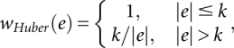where k = 1.345σ and σ is the standard deviation of the errors from the mean model that can be estimated by median absolute residual divided by 0.6745, and e is the residual value.

One of the key assumptions in Equation 1 is that the variances of the error terms are equal for all observations. When constant variance assumption is substantially violated, it may give less efficient estimates of array and probe effects and misleading standard errors. Figure 1 shows a plot of residual versus predicted values, where the residual variance is clearly a function of the predicted values. To accommodate the potential heteroscedasticity, we introduce a dispersion generalized linear model (GLM).

Defining var(ε_ij) = υ_ij, in principle, we can take into account the variance of residuals by considering the weight w_new = w_Huberυ_ij⁻¹, where more weight is assigned to those observations having smaller variance of residuals. In general, the dispersion GLM can be expressed as

where υ_ij is the observed variance of residuals from the mean model (1), g(·) is the link function, γ_i is the ith array effect for i = 1,…,n; κ_j is the jth probe effect for j = 1,…,J; B is the vector of parameters consisting of mean, array, and probe effects. This model gives us estimates of variance for the mean model (1). A robust version of the GLM is used to deal with potential outliers, with robust weights derived using the first quantile of residuals from dispersion model (2). Thus, the resulting prior weights using fitted values from the dispersion model are

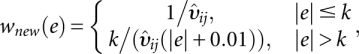where is the estimated dispersion value.

The model can be fitted iteratively using two interconnected iterative weighted least square (IWLS):

1. Given the dispersion predicted value incorporated into prior weight, use IWLS to update  for the mean model. The updating equation is

   

   where ∑⁻¹ is a diagonal matrix with elements .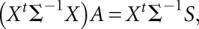
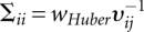2. Given Â, use IWLS to update with the squared of residuals ɛ² from the mean model as response data. The updating equation is

   

   where D⁻¹ is a diagonal matrix with elements being the weights in current dispersion model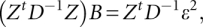

   

   where r is the residual value in current dispersion model and Q1 is the first quantile of residuals.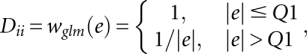

3. Iterate Steps 1 and 2 until convergence.

The array effects are captured by the χ² statistic, computed by

where is a vector of estimated array effects, and is its estimated covariance matrix. These quantities are available from the robust linear model fit. The covariance matrix can be estimated based either on the sandwich form of weighted covariance matrix I⁻¹JI⁻¹, where I is the observed Fisher information and J is the variance of the estimating function (Pawitan 2001), or the asymptotic form

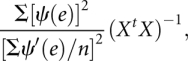where n is the number of residuals and ψ(e) is defined as [w(e)]e (Huber 1964).

The ideal LVS miRNAs are those with the least array-to-array variability. This means that when we compare the χ² statistics among the miRNAs, those with smaller values are more likely to become LVS miRNAs. A nonparametric quantile regression is then fitted to χ² values as a function of the residual SDs, since the value of the statistics is also determined by the residual variance. The relationship can be seen graphically in the scatter plot of the square-root or logarithm of array effect versus the logarithm of the residual SD. Points below the curve fitted by the quantile regression model are used as the reference set for normalization. The user is allowed to set the proper quantile (τ) value to fit.

For mRNA it has been known for a long time that at most eucaryotic cells express ∼30%–40% of the genes (Su et al. 2002; Jongeneel et al. 2003) and even less are likely to be differentially expressed among clinical conditions. On the other hand, it is less clear how miRNA are expressed in normal or experimental conditions. According to some experimental data, it is reasonable to expect ∼60% of miRNAs to remain constant between experimental conditions (Volinia et al. 2006; Yanaihara et al. 2006). Some steps of the normalization procedure, in particular the calibration step based on VSN, might be affected by a small number of features, as the case in miRNA array. Therefore, we suggest setting τ to a proportion around 70%, unless prior biological knowledge suggests setting a different threshold. As the number of miRNAs increases it will be possible to have a better tuning of this parameter.

Ideally, those LVS miRNAs should not only have a small array effect but also retain the most useful information and be representative of the signal level of the other miRNAs. In the case where most of the selected LVS miRNAs happen to come from those with low intensity, the algorithm allows one to stratify by level of intensity, and choose a certain proportion of LVS miRNAs from each stratum. This option solves the problem of possible information loss due to a restricted range of intensities.

Normalization on the LVS miRNAs

Once the LVS miRNAs are identified, the normalization is performed using VSN (Huber et al. 2002), where transformation parameters are estimated from the LVS miRNAs. Briefly the VSN procedure first calibrates sample-to-sample variations so that data are on a common scale and have a common distribution. After that, variance stabilization based on a parametric arcsinh (inverse of hyperbolic sine) transformation is performed to address the dependence of the variance on the mean intensity. An alternative normalization procedure based on a spline smoother between the individual array and an arbitrary reference array can be used also. The reference array may be a pseudo-median array or any user-specified array. The curve fitted through the LVS miRNAs is then used to map intensities of all the miRNAs in each array to normalized values. This step is single-array based, in contrast to the multiarray basis in the step of identifying LVS.

The current implementation of LVS allows the user to normalize data at the probe level prior to other preprocessing procedures, or the miRNA level, i.e., after summarization of probe-level data into the miRNA level. For all analysis in this paper, normalization based on LVS features is applied at the miRNA level: the summarized value is given by the array effect from model (1) (hereafter called the RLM summarization). Unless explicitly stated, we set the proportion parameter or the so-called quantile threshold to 70% in LVS normalization based on VSN.

Software

All the analyses are performed using the R (R Development Core Team 2009) and Bioconductor (Gentleman et al. 2004) software. We have developed an R package called LVSmiRNA, freely available with a vignette from the author website (www.med.unibs.it/∼calza) and the Bioconductor website at http://bioconductor.org. The normalization procedure is highly computationally intensive due to the iterative nature of the fitting algorithm. To get an optimal implementation, the package is coded in C and can take advantage of the multicore hardware architecture that allows parallel computation. On an eight-core machine (dual Intel Pentium QuadCore Xeon 2.27 GHz) the selection of invariant-set features takes ∼30 sec for a data set with 41 samples and 534 miRNAs (overall 11,061 probes) using joint modeling, and only 4 sec for a standard RLM.

Data sets and comparison procedures

Two data sets produced on Agilent platforms are used to illustrate and validate the proposed normalization procedure, and to compare it with other methods.

Spike-in data

This data set is derived from a library of synthetic RNA sequences, corresponding to human mature miRNAs as well as in-house miRNAs with particularly similar sequences hybridized on an Agilent Human miRNA Microarray 2.0 (Willenbrock et al. 2009). The individual array data as well as the actual synthetic miRNA concentrations are downloaded from Genome Expression Omnibus (GEO) database under the series accession number GSE14511. The downloaded data consist of a total of 799 miRNA species (excluding control features) for four samples organized in two groups A and B. Out of 799 miRNAs, 102 are not spiked-in, 524 have a true fold-change (FC) level ranging from 0.0625 to 16-fold, while a set of 173 miRNA (24.8%) species have a constant FC level of 1. These FC1 miRNAs are the ideal reference set for normalization.

Normal-tissue microarray data

These data are produced as part of a comparison between microarray and quantitative TaqMan real-time PCR (qPCR) measurements (Ach et al. 2008). The data set consists of 43 samples hybridized on an Agilent Human miRNA Microarray 1.0 coming from nine different human tissues (brain, breast, heart, liver, placenta, testis, ovary, skeletal muscle, and thymus). There are four to five arrays for each tissue type, and each array contains 534 miRNAs (excluding control probes). Sixty miRNAs are profiled with RT-PCR on every tissue (only the within-tissue average value is available). Data are available from GEO with series number GSE11879.

Normal-tissue RT-PCR data

In a study on the processing patterns of miRNA, Lee et al. (2008) profile the expression of 202 mature miRNAs using qPCR from 22 different human tissues. Expression values are transformed using arcsinh transformation to allow for the presence of zeros. Except for breast tissues, all the tissue types measured by Ach et al. (2008) are available in this data set. The availability of the RT-PCR data allows us to compare different tissue types, while knowing the true fold change of a large number of miRNAs.

Comparative procedures

For the spike-in data we can compare LVS to the ideal normalization based on the FC1 miRNAs. We further compare the performance of LVS normalization to no normalization, 75th percentile shift, quantile, inv-P, global median, VSN, and locally weighted scatter-plot smoothing (lowess) normalization methods. The percentile-shift normalization is the recommended normalization by Agilent (Agilent 2008) for its miRNA platform. It equalizes the 75th percentile of the distribution of each sample, setting it to an arbitrary value. Similarly, global median normalization makes median equal across samples. The quantile normalization (Wernisch et al. 2003) is a commonly used algorithm that equalizes sample intensity distributions to an arbitrary reference one. The inv-P method (Pradervand 2009) is a modification of the invariant-set normalization procedure. Briefly, it selects invariant features among those with high average intensity and low variability, or low SD. The algorithm first removes the mean versus SD trend and then fits a mixture model to the mean and corrected SD distributions in order to identify a cluster of features with high average intensity and low SD. The lowess normalization is an intensity-dependent procedure, where the log-ratio for each sample is adjusted by the fitted value from robust weighted least squares.

All the normalization methods except LVS are performed on values preprocessed according to Agilent's default signal, Total Gene Signal. To allow for the presence of negative values and to make them comparable with the transformation used by VSN, data are transformed on the arcsinh scale.

REFERENCES

- Ach R, Wang H, Curry B 2008. Measuring microRNAs: Comparisons of microarray and quantitative PCR measurements, and of different total RNA prep methods. BMC Biotechnol 8: 69 doi: 10.1186/1472-6750-8-69 [DOI] [PMC free article] [PubMed] [Google Scholar]
- Agilent 2008. Agilent miRNA data import guide. Agilent, Santa Clara, CA [Google Scholar]
- Betel D, Wilson M, Gabow A, Marks D, Sander C 2008. MicroRNA target predictions with expression profiles. Nucleic Acids Res 36: 149–153 [DOI] [PMC free article] [PubMed] [Google Scholar]
- Calza S, Valentini D, Pawitan Y 2007. Normalization of oligonucleotide arrays based on the least-variant set of genes. BMC Bioinformatics 140: 5–9 [DOI] [PMC free article] [PubMed] [Google Scholar]
- Davison TS, Johnson CD, Andruss BF 2006. Analyzing micro-RNA expression using microarrays. Methods Enzymol 411: 14–34 [DOI] [PubMed] [Google Scholar]
- Edwards D 2003. Non-linear normalization and background correction in one-channel cDNA microarray studies. Bioinformatics 19: 825–833 [DOI] [PubMed] [Google Scholar]
- Fabbri M, Croce CM, Calin GA 2008. MicroRNAs. Cancer J 14: 1–6 [DOI] [PubMed] [Google Scholar]
- Gentleman RC, Carey VJ, Bates DM, Bolstad B, Dettling M, Dudoit S, Ellis B, Gautier L, Ge Y, Gentry J, et al. 2004. Bioconductor: Open software development for computational biology and bioinformatics. Genome Biol 5: R80 doi: 10.1186/gb-2004-5-10-r80 [DOI] [PMC free article] [PubMed] [Google Scholar]
- Griffiths-Jones S 2004. The MicroRNA Registry. Nucleic Acids Res 32: D109–D111 [DOI] [PMC free article] [PubMed] [Google Scholar]
- Griffiths-Jones S, Grocock R, van Dongen S, Bateman A, Enright A 2006. MiRBase: MicroRNA sequences, targets and gene nomenclature. Nucleic Acids Res 34: D140–D144 [DOI] [PMC free article] [PubMed] [Google Scholar]
- Griffiths-Jones S, Saini H, van Dongen S, Enright A 2008. MiRBase: Tools for microRNA genomics. Nucleic Acids Res 36: D154–D158 [DOI] [PMC free article] [PubMed] [Google Scholar]
- Guarnieri D, DiLeone R 2008. MicroRNAs: A new class of gene regulators. Ann Med 40: 197–208 [DOI] [PubMed] [Google Scholar]
- Hua YJ, Tu K, Tang Z, Li Y, Xiao H 2008. Comparison of normalization methods with microRNA microarray. Genomics 92: 122–128 [DOI] [PubMed] [Google Scholar]
- Huber PJ 1964. Robust estimation of a location parameter. Ann Math Stat 35: 73–101 [Google Scholar]
- Huber W, von Heydebreck A, Sultmann H, Poustka A, Vingron M 2002. Variance stabilization applied to microarray data calibration and to the quantification of differential expression. Bioinformatics 18: S96–S104 [DOI] [PubMed] [Google Scholar]
- Irizarry R, Hobbs B, Collin F, Beazer-Barclay Y, Antonellis K, Scherf U, Speed T 2003. Exploration, normalization, and summaries of high density oligonucleotide array probe level data. Biostatistics 4: 249–264 [DOI] [PubMed] [Google Scholar]
- Jongeneel CV, Iseli C, Stevenson BJ, Riggins GJ, Lal A, Mackay A, Harris RA, O'Hare MJ, Neville AM, Simpson AJG, et al. 2003. Comprehensive sampling of gene expression in human cell lines with massively parallel signature sequencing. Proc Natl Acad Sci 100: 4702–4705 [DOI] [PMC free article] [PubMed] [Google Scholar]
- Kiss T 2002. Small nucleolar RNAs: An abundant group of noncoding RNAs with diverse cellular functions. Cell 109: 145–148 [DOI] [PubMed] [Google Scholar]
- Koenker R 2007. Quantreg: Quantile Regression. R package version 4.06 [Google Scholar]
- Koenker R, Bassett G 1978. Regression quantiles. Econometrica 46: 33–50 [Google Scholar]
- Lee PD, Sladek R, Greenwood CM, Hudson TJ 2002. Control genes and variability: Absence of ubiquitous reference transcripts in diverse mammalian expression studies. Genome Res 12: 292–297 [DOI] [PMC free article] [PubMed] [Google Scholar]
- Lee Y, Nelder J, Pawitan Y 2006. Generalized linear models with random effects. Chapman and Hall, London [Google Scholar]
- Lee E, Baek M, Gusev Y, Brackett DJ, Nuovo G, Schmittgen T 2008. Systematic evaluation of microRNA processing patterns in tissues, cell lines, and tumors. RNA 14: 35–42 [DOI] [PMC free article] [PubMed] [Google Scholar]
- Li C, Wong WH 2001. Model-based analysis of oligonucleotide arrays: Expression index computation and outlier detection. Proc Natl Acad Sci 98: 31–36 [DOI] [PMC free article] [PubMed] [Google Scholar]
- Pasquinelli AE, Hunter S, Bracht J 2005. MicroRNAs: A developing story. Curr Opin Genet Dev 15: 200–205 [DOI] [PubMed] [Google Scholar]
- Pawitan Y 2001. In all likelihood: Statistical modeling and inference using likelihood. Oxford University Press, New York [Google Scholar]
- Pradervand S 2009. Impact of normalization on miRNA microarray expression profiling. RNA 15: 493–501 [DOI] [PMC free article] [PubMed] [Google Scholar]
- R Development Core Team. 2009. R: A language and environment for statistical computing. R Foundation for Statistical Computing, Vienna, Austria [Google Scholar]
- Rao Y, Lee Y, Jarjoura D, Ruppert A, Liu C, Hsu J, Hagan J 2008. A comparison of normalization techniques for microRNA microarray data. Stat Appl Genet Mol Biol 7: 22 doi: 10.2202/1544-6115.1287 [DOI] [PubMed] [Google Scholar]
- Ritchie ME, Silver J, Oshlack A, Holmes M, Diyagama D, Holloway A, Smyth GK 2007. A comparison of background correction methods for two-colour microarrays. Bioinformatics 23: 2700–2707 [DOI] [PubMed] [Google Scholar]
- Smyth GK 2004. Linear models and empirical Bayes methods for assessing differential expression in microarray experiments. Stat Appl Genet Mol Biol 3: 3 doi: 10.2202/1544-6115.1027 [DOI] [PubMed] [Google Scholar]
- Su AI, Cooke MP, Ching KA, Hakak Y, Walker JR, Wiltshire T, Orth AP, Vega RG, Sapinoso LM, Moqrich A, et al. 2002. Large-scale analysis of the human and mouse transcriptomes. Proc Natl Acad Sci 99: 4465–4470 [DOI] [PMC free article] [PubMed] [Google Scholar]
- Tseng G, Oh M, Rohlin L, Liao J, Wong W 2001. Issues in cDNA microarray analysis: quality filtering, channel normalization, models of variations and assessment of gene effects. Nucleic Acids Res 29: 2549–2557 [DOI] [PMC free article] [PubMed] [Google Scholar]
- Volinia S, Calin GA, Liu CG, Ambs S, Cimmino A, Petrocca F, Visone R, Iorio M, Roldo C, Ferracin M, et al. 2006. A microRNA expression signature of human solid tumors defines cancer gene targets. Proc Natl Acad Sci 103: 2257–2261 [DOI] [PMC free article] [PubMed] [Google Scholar]
- Wang B, Wang XF, Howell P, Qian X, Huang K, Riker AI, Ju J, Xi Y 2010. A personalized microRNA microarray normalization method using a logistic regression model. Bioinformatics 26: 228–234 [DOI] [PubMed] [Google Scholar]
- Wernisch L, Kendall S, Soneji S, Wietzorrek A, Parish T, Hinds J, Butcher P, Stoker N 2003. Analysis of whole-genome microarray replicates using mixed models. Bioinformatics 19: 53–61 [DOI] [PubMed] [Google Scholar]
- Willenbrock H, Salomon J, Barken KIMB, Nielsen FC, Litman T 2009. Quantitative miRNA expression analysis: Comparing microarrays with next-generation sequencing. RNA 15: 2028–2034 [DOI] [PMC free article] [PubMed] [Google Scholar]
- Yanaihara N, Caplen N, Bowman E, Seike M, Kumamoto K, Yi M, Stephens RM, Okamoto A, Yokota J, Tanaka T, et al. 2006. Unique miRNA molecular profiles in lung cancer diagnosis and prognosis. Cancer Cell 9: 189–198 [DOI] [PubMed] [Google Scholar]
- Yang YH, Dudoit S, Luu P, Lin D, Peng V, Ngai J, Speed T 2002. Normalization for cDNA microarray data: A robust composite method addressing single and multiple slide systematic variation. Nucl Acids Res 30: e15 doi: 10.1093/nar/30.4.e15 [DOI] [PMC free article] [PubMed] [Google Scholar]
- Zhao Y, Wang E, Liu H, Rotunno M, Koshiol J, Marincola F, Landi M, McShane L 2010. Evaluation of normalization methods for two-channel microRNA microarrays. J Transl Med 8: 69 doi: 10.1186/1479-5876-8-69 [DOI] [PMC free article] [PubMed] [Google Scholar]