Dating Primate Divergences through an Integrated Analysis of Palaeontological and Molecular Data

Abstract

Estimation of divergence times is usually done using either the fossil record or sequence data from modern species. We provide an integrated analysis of palaeontological and molecular data to give estimates of primate divergence times that utilize both sources of information. The number of preserved primate species discovered in the fossil record, along with their geological age distribution, is combined with the number of extant primate species to provide initial estimates of the primate and anthropoid divergence times. This is done by using a stochastic forwards-modeling approach where speciation and fossil preservation and discovery are simulated forward in time. We use the posterior distribution from the fossil analysis as a prior distribution on node ages in a molecular analysis. Sequence data from two genomic regions (CFTR on human chromosome 7 and the CYP7A1 region on chromosome 8) from 15 primate species are used with the birth–death model implemented in mcmctree in PAML to infer the posterior distribution of the ages of 14 nodes in the primate tree. We find that these age estimates are older than previously reported dates for all but one of these nodes. To perform the inference, a new approximate Bayesian computation (ABC) algorithm is introduced, where the structure of the model can be exploited in an ABC-within-Gibbs algorithm to provide a more efficient analysis.

Fossil evidence is the only direct source of information about long-extinct species and their evolution. Morphological similarities between extant species and fossil remains are used to infer the existence of ancestral species during the geological period to which the fossil is allocated. Conditional on there being no classification or dating error, the fossil's age provides a minimum bound for the divergence time of the evolutionary lineage it represents.

Sequence data from extant species provide an indirect source of information about evolutionary history. The pattern and variability observed in homologous sequences of DNA from different species contain traces of the history of the divergence and evolution of the phylogeny, and mathematical models of evolution can be used to combine our knowledge of genetics with the sequence data to extract information about evolutionary history, particularly divergence times. Many methods and models have been proposed with this aim, but all rely in some way on fossil evidence, as an external source of information must be used to calibrate the substitution rate. Fossil evidence is used to provide initial estimates for node ages in phylogenetic trees, which are then updated in light of molecular evidence. Yang and Rannala (2006) found that, for divergence time estimates based on sequence data, the largest source of uncertainty came from the fossil calibration dates used.

Although fossils provide good explicit minimum bounds on the age of a clade, maximum bounds need to be inferred rather than measured and thus are inherently uncertain. Uncertainty about a maximum bound on the node age has been dealt with in various ways in molecular analyses, typically by relying upon a subjective judgement about the node age based on the age of the oldest fossil (i.e., a maximum bound, or the weight of the tail in a more general prior distribution).

In this paper, we use a database of recorded fossil species combined with a model of speciation to find a model-based estimate of node ages. These estimates are then used as prior distributions for estimating molecular divergence times. The benefit of introducing an element of process modeling into the analysis of the fossil record is that it moves the subjective judgements further from important quantities and allows us to utilize more of the fossil record, thus letting data play a larger role in the analysis. In determining the expected gap between the age of the oldest fossil and the divergence time, a key influence is exerted by rates of fossil preservation and discovery, which are unknown and believed to vary through time (e.g., Foote et al. 1999, Smith.et al 2002, Tavare.et al 2002, Soligo.et al 2007, Paul.2009). We use the pattern of species diversity through the Cenozoic and the number of extant primate species to estimate the sampling rate and the divergence time of the primates. The posterior distributions from the fossil analysis are used as the prior distribution in the molecular analysis to estimate a posterior distribution for the divergence time that uses both the fossil and molecular records more fully than previous analyses.

The paper is organized as follows. The first section describes the analysis of the fossil record. The following section contains the molecular analysis and the final section contains a discussion. The details of the inference procedure used in the analysis of the fossil data are given in the Appendix, where we introduce a new variant on the Markov chain Monte Carlo (MCMC)–approximate Bayesian computation (ABC) (Marjoram et al. 2003) algorithm in order to improve the efficiency of our analysis.

USING THE FOSSIL RECORD

Fossil calibrations are essential when dating evolutionary events. Even if the analysis primarily uses molecular data, fossil evidence is used to provide prior distributions for one or more nodes in the phylogeny. This information is then used to calibrate the molecular clock and thus has consequences for estimation of other node ages. Early analyses using the molecular clock to date divergence times typically treated the oldest fossil representative as if it estimated the age of the node without error (Graur and Martin 2004, Hedges.et al 2004). This progressed to introducing uncertainty by specifying a range of possible values with hard bounds representing the limits of the uncertainty (Thorne et al. 1998), with zero probability assigned to ages outside of this range. Fossil evidence is well suited to providing a good hard minimum bound on the age of a node based on the oldest fossil representative, with the level of accuracy limited only by the accuracy of taxonomic assignment of the fossil and of the dating procedure used. However, the fossil record does not directly give any information regarding a maximum bound on the age (Benton and Donoghue 2007, Steiper.Young 2008). Thus, hard bounds are often either overconfident, where they are set too low, or too conservative, where unrealistically high maximum bounds are used. Yang and Rannala (2006) moved beyond the use of uniform distributions for calibration dates to allow general prior distributions, which can incorporate more information about the calibration age. These allow for most of the probability to be placed on dates near to the minimum bound, but with long tails to account for the a priori unlikely event that the node age is actually much older than the fossil evidence suggested. They chose prior distributions by fitting a parametric form (a gamma distribution) to estimated maximum and minimum bounds on the node age, allowing for 5% uncertainty outside this range.

However, the fossil record contains more information about a node age than that contained solely in the oldest fossil ascribed to a particular lineage. The age of the oldest fossil may be the single most informative piece of data, but other parts of the record can help reduce the uncertainty in any estimate and provide a more nuanced picture. By considering more of the fossil record, we can move from using prior distributions based on the oldest fossil to distributions based on a wider appreciation of the fossil record and its underlying processes. The distribution of fossil ages contains information about the diversity (number of species) of a phylogeny through time. When combined with extant diversity counts, this can be used to infer the sampling rate or completeness of the fossil record (Tavaré et al. 2002, Soligo.et al 2007, Wilkinson.Tavare 2009). For periods and phylogenies with high sampling rates, we expect the age of the oldest known fossil to be close to the divergence time of the phylogeny, whereas if the sampling rate is low, we expect the range of values possible for the gap between the oldest fossil and the root of the phylogeny it represents to be much more variable. For terrestrial vertebrates, the completeness (the proportion of species that have been preserved and then discovered in the fossil record) is generally believed to be low. For example, Martin (1993) and Tavaré et al. (2002) estimate the completeness of the primate fossil record to be less than 7% compared with an estimate of 29% for dinosaurs (Wang and Dobson 2006).

Model for the Fossil Data

The model for the fossil data can be thought of in two parts: 1) speciation and 2) fossilization and recovery. The speciation model describes the growth of the number of species (the diversity) from a common ancestor to the observed extant diversity, whereas the fossilization and recovery model describes how the phylogeny is recorded in the known fossil record.

To model speciation, we use a continuous-time inhomogeneous binary Markov branching process (Harris 1963). To aid description, we use the language of family trees and refer to the direct descendants of a species as its offspring. Let Z(t) denote the number of species extant at time t, where t = 0 denotes the present. The age of the oldest known fossil representative is used as an absolute minimum bound on the age of the clade. The root of the tree is placed at this age plus τ million years, where τ represents the temporal gap between the oldest primate fossil and the primate divergence time. We assume that two species are present at this time and that each species lives for an exponentially distributed period of time with mean 1/λ before becoming extinct. Upon its extinction, at time t say, it is replaced by either zero or two new species with probability p₀(t) or p₂(t) = 1 − p₀(t), respectively. The birth and death probabilities p₀(t) and p₂(t) can be determined by fixing a parametric form for the expected population size at time t, that is, 𝔼Z(t) = f(t;ψ), where ψ are unknown parameters to be estimated. We initialize the branching process with two species, and consider the tree to have two sides, corresponding to Haplorhini and Strepsirrhini in the primate phylogeny. Because the root of the tree represents the crown divergence time, we require both sides of the tree to be present at time t = 0, modeling the fact that there are extant Haplorhini and Strepsirrhini. We condition both sides of the tree on nonextinction by using rejection sampling (Ripley 1987), by simply disregarding simulations that go extinct on either side of the tree. Note that if we do not condition on nonextinction, we would be modeling a point of divergence along the stem lineage, defined by the taxa included in the fossil data, rather than the crown divergence time (Soligo et al. 2007).

This model provides simulated numbers of species extant through time, given a value for the crown divergence time. To simulate sample fossil data sets, we introduce two different observation models, a simple binomial model and a more complex Poisson sampling model. Note that it is not possible to date fossils precisely. The fossil data shown in Table 1 are resolved at the epochal level, and for each epoch, we have counts of the number of generally recognized primate morphospecies known to have lived during that epoch. Our observation models simulate the number of fossils discovered in each of the 14 epochs in the Cenozoic {D_i}_{i = 1}¹⁴ given the number of species {N_i}_{i = 1}¹⁴. In the binomial model, each species in epoch i has probability α_i of being preserved and then discovered as a fossil, regardless of the length of time the species was extant. This gives D_i∼Binomial(N_i,α_i), where N_i is the number of species extant during any part of epoch i.

TABLE 1.

A summary of the number of crown group primate and crown group anthropoid species known from the fossil record (Tavaré et al. 2002; Soligo et al. 2007)

Epoch	k	Time at base of interval k (Ma)	Primate fossil counts, 𝒟	Anthropoid fossil counts, 𝒜
Extant	0		376	281
Late Pleistocene	1	0.15	22	22
Middle Pleistocene	2	0.9	28	28
Early Pleistocene	3	1.8	30	30
Late Pliocene	4	3.6	43	40
Early Pliocene	5	5.3	12	11
Late Miocene	6	11.2	38	34
Middle Miocene	7	16.4	46	43
Early Miocene	8	23.8	34	28
Late Oligocene	9	28.5	3	2
Early Oligocene	10	33.7	22	6
Late Eocene	11	37.0	30	2
Middle Eocene	12	49.0	119	0
Early Eocene	13	54.8	65	0
Pre-Eocene	14		0	0

Notes: Time during the Cenozoic is divided into 14 geologic epochs, with the dates for each epoch given in the table as millions of years ago. Also given is the extant diversity (Groves 2005). Note that the geological scale used here does not take account of the latest adjustments made to the age of the Pliocene–Pleistocene transition (International Commission on Stratigraphy 2009).

The Poisson model assumes that each species present in any given epoch has an equal probability of being discovered as a fossil for each year it is extant. Consequently, longer-lived species will have a higher probability of preservation and discovery than shorter-lived species. Assume that fossil finds occur along the branches present in epoch i as the points of a Poisson process of rate β_i. Each species is recorded at most once during an epoch, regardless of whether there are multiple points along its branch, so that a species that lived for duration t in epoch i has probability 1 − e ^{− β_it} of being discovered in the fossil record during that epoch. It is known that the rates of fossil preservation and discovery have varied through time, for example, because rocks from different geological epochs are not present in accessible locations in equal abundance (Raup 1976, Peters and Foote 2001, Smith.et al 2002, McGowan.et al 2008). Added to this are complications regarding sampling locations (Western Europe and North America are better sampled than Africa or Asia, for instance) and variation in habitable latitudes as climate and the availability of dispersal routes changed through time. For example, primates are thought to have originated in more southern latitudes, spreading northward at the beginning of the Eocene, and again in the Miocene, as a result of globally warmer climates (and of developing land bridges in the case of the Miocene), whereas retreating from more northern latitudes as a result of climate cooling, for example, toward the end of the Eocene and beginning of the Oligocene (e.g., Krause and Maas 1990, Martin 1993, Soligo and Martin 2006, Andrews and Kelley 2007, Martin et al. 2007, Soligo 2007). For this reason, we allow the observation process to vary in intensity between epochs and write α = (α₁,α₂,…,α₁₄) and β = (β₁,…,β₁₄).

Both the binomial and Poisson sampling models are phenomenological in nature, rather than process models of the complex underlying processes. Fossil deposition and preservation rates will depend on a variety of factors for each species, such as habitat, location, and population size. Similarly, the classification of fossils and the identification of new species are processes prone to error, with opinions over dates and classifications changing over time. It would be hard to model all these processes as the data available for parameter estimation are limited. Instead, we use simple statistical models that try to approximate the net effect of the interaction of the various processes in order to find a mathematical description of the observations without paying too much attention to the individual processes.

An important extension to this model is to consider the effect of the mass-extinction event that took place at the Cretaceous–Tertiary (K-T) boundary 65 Ma (1 Ma = 10⁶ years ago). There is no direct fossil evidence as to whether primates existed during the Cretaceous, so the importance of the K-T boundary when dating the divergence time is unclear. However, if primates lived at this time, it is highly likely that they were also affected by the event. We can include the effect of the K-T crash by making each species in the simulation extinct with probability p at the K-T boundary at t = − 65 Myr. Extinctions are assumed to occur independently for each species, and we assume that species wiped out at the K-T boundary have no offspring. Thus, the diversity in the simulation just after the K-T boundary has a binomial distribution with parameters (n,p) = (Z( − 65),p). We treat p as an unknown parameter and estimate it in the inference. We estimate the divergence time both with and without (p = 0) the K-T crash model to examine its importance.

Inference

The previous section described the forwards model, a stochastic mapping from unknown parameters θ: = (τ,ψ,β,α,λ,p) to sample fossil data sets {D_i}_{i = 1}¹⁴. The model is stochastic and any particular combination of parameters can lead to a wide variety of behavior. To estimate divergence times, we must solve the inverse problem and use the fossil observations 𝒟_obs and the number of extant species N₀ to learn the unknown parameters. We use a Bayesian approach and give all unknown parameters prior distributions (described in the Results section) and then find the posterior distribution of the parameters given the data, denoted π(θ|𝒟).

Inference using this model is difficult and requires nonstandard methods because the likelihood function l(θ;𝒟_obs) = ℙ(𝒟_obs|θ) is unknown (Kendall 1948). Without an explicit mechanism for calculating the likelihood, standard inference approaches such as MCMC or importance sampling are not possible. Instead, we use a “likelihood-free” approach, known as ABC (Beaumont et al. 2002, Marjoram.et al 2003, Sisson.et al 2007).

The main idea behind ABC is sufficient for understanding our inference approach. The simplest ABC algorithm is based upon the rejection algorithm. We draw parameter θ from its prior distribution, simulate sample data 𝒟 using this parameter setting, and accept the parameter into our sample if the simulated data are a close approximation to the observed data. To define “close,” we require a metric ρ(·,·) on the state space and a tolerance ϵ and we accept θ if ρ(𝒟,𝒟_obs) ≤ ϵ.

This algorithm is not exact. Accepted θ values do not form a sample from the posterior distribution π(θ|𝒟), but from some distribution that is an approximation to it, where the accuracy of the algorithm depends on ρ and the tolerance ϵ. The tolerance ϵ represents a trade-off between computability and accuracy; large ϵ values will mean more acceptances and will enable us to generate samples more quickly, but the distribution obtained may be a poor approximation to π(θ|𝒟). Small ϵ values will mean that the approximation is more accurate, but the acceptance rate will be lower and so we will require more computer time to generate a sample of a given size. To choose a value of ϵ, we must make a compromise between the time and computer power available and the desired accuracy. Our choice of metric and tolerance are given in the Results section.

The standard ABC approach cannot be applied directly to the problem here, as the number of unknown parameters is too large, and so any naive search of the parameter space will spend most of its time in regions of low posterior probability. Instead, we use a more efficient approach and develop an ABC-within-Gibbs sampler that exploits some of the known model structure. Details are given in the Appendix.

Dating multiple divergence times.—

The primate fossil record is poor and is limited in its ability to constrain estimates of divergence times. However, by using as much of the record as possible, we can hope to constrain the estimates more than would be possible solely using the age of the oldest fossil ascribed to a lineage. Morphological detail in the fossils is used to classify each fossil into a subgroup of species and this information can be used to date multiple divergence times simultaneously. We estimate the joint distribution of the crown primate and anthropoid divergences using an optimal subtree selection (OSS) algorithm. The fossil data set in Table 1 contains two sets of numbers. The first grouping gives the number of crown primate species discovered, 𝒟_obs = (D₁,…,D₁₄), whereas the second grouping gives the number of crown anthropoid species, 𝒜_obs = (A₁,…,A₁₄). Notice that D_k ≥ A_k for all k, as anthropoids are a subset of the primates. We let τ denote the temporal gap between the oldest primate fossil and the last common ancestor (LCA) of the extant primates and let τ^* denote the temporal gap between the oldest anthropoid (platyrrhine–catarrhine) fossil and the LCA of the anthropoids. Our approach to inferring τ^* is based on finding the subtree with fossil counts that most closely match the anthropoid fossil counts 𝒜_obs. If the distance between simulated and real anthropoid fossil counts ρ(𝒜_obs,𝒜) is less than tolerance ϵ₂, we measure the temporal gap from the base of this subtree to the start of the late Eocene interval. This is then our estimate for τ^*. We require that the root of the subtree (the death time of the anthropoid LCA) occurs earlier than the beginning of the late Eocene, 37 Ma. We must also condition the subtree on nonextinction and check that both branches leading from the subtree root have extant descendants, as one side of the subtree represents the Platyrrhini and the other the Catarrhini and both these groups have extant representatives. We refer to this approach as OSS. A rejection-based ABC algorithm for inference would be:

Optimal Subtree Selection (OSS)

1. Draw parameters θ = (τ,α,ψ,p,λ) from π(·).

2. Simulate a tree and fossil finds using parameter θ. Count the number of simulated fossils in each interval, 𝒟^′ = (D₁^′,…,D₁₄^′).

3. Calculate the value of the metric ρ(𝒟_obs,𝒟^′). If

   (1)

4. Perform an exhaustive search of all possible subtrees. For each subtree, check that the root of the subtree occurs at least 37 Ma and that both offspring of this root produce trees that survive to the present. If both conditions are met, count the number of fossils on the subtree, 𝒜^′ = (A₁,…,A₁₄).

5. Determine which subtree has the smallest value of ρ(𝒜_obs,𝒜^′), that is, has fossil counts closest to the anthropoid fossil set. This is the “optimal subtree.” If

   (2)

In practice, this algorithm is too inefficient to give sensible results in a reasonable time, as repeatedly drawing from the prior distribution means that a long time is spent simulating data with parameter values that lie in the tails of the posterior distribution. A more efficient algorithm is given in the Appendix. Note that this algorithm requires the genealogy to be simulated rather than just keeping track of Z(t) as is sufficient in a birth–death process.

The division of the data into two nested parts (primates and anthropoids) is not a necessary part of the analysis, but it is done to maximize the information that can be extracted from the data. It is possible to consider just the primate fossil counts 𝒟 and estimate only the primate divergence time by stopping the algorithm after Step 3. An alternative approach to estimating multiple divergence times not based on the OSS algorithm is given in Wilkinson and Tavaré (2009).

Data and Results

The primate fossil data set is given in Table 1. It contains counts of the number of primate and anthropoid species discovered in each epoch during the Cenozoic. The anthropoids are a monophyletic subgroup of the primates containing the hominoids (apes and humans) and the New and Old World monkeys. Because fossils cannot be precisely dated, we bin the data into geological epochs and count the number of species discovered coming from each epoch. Note that so far no undoubted primate fossil older than 54.8 Myr has been discovered and no crown group anthropoid fossil older than 37 Myr. Also included in the table are the numbers of known extant species, taken from Groves (2005). Information on extant diversity is valuable as it gives information about the sampling rates that is otherwise difficult to estimate.

Before giving the results of the analysis, we need to make various implementation assumptions. First, the birth and death probabilities p₀(t) and p₂(t) need to be specified through time. This is done by fixing the expected growth to be logistic, so that

(3)

for unknown γ and ρ. We can use the result that

(4)

(see, e.g., Harris 1963) to equate the expected growth curve to the birth and death probabilities to solve for p₀(t) and p₂(t). Other simple functional forms for the growth were tried (results not shown), but it is possible to show using Bayes factors (approximated by the acceptance probability in the ABC algorithm) that logistic growth is best supported by the data (Wilkinson 2007).

We give prior distributions to all unknown parameters except τ^*, which is chosen by an optimality criterion during the simulation. The prior distributions used are

The prior on τ is equivalent to assigning a uniform prior distribution on the interval [154.8,54.8] Ma for the primate divergence time t₁, which represents our prior state of uncertainty about the primate divergence. The prior range for 1/λ was set by consideration of the mean species survival time (Alroy 1994), and the range for ρ and λ were fixed by considering the mean diversity implied by the logistic growth curve (Wilkinson 2007). Prior distributions for α and β are chosen for reasons of conjugacy. For the binomial model, we let α_i∼U[0,1] and assume that the α_i are independent a priori. In the Poisson model, we use gamma prior distributions, setting β_i∼G(5,50) for i = 1,…,14 with the β_i independent a priori, where G(a,b) denotes the gamma distribution with shape parameter a and rate parameter b (i.e., if X∼G(a,b) the density of X is x^{a − 1}b^ae ^{− bx}/Γ(a)). When we use the K-T crash model, we give the unknown probability of extinction, p, a U[0,0.5] distribution. The posteriors for τ and τ^* appear to be robust to small changes in the prior specifications of all the parameters.

The ABC inference procedure requires a choice of metric ρ(·,·) and a tolerance ϵ. After investigation into the choice of metric (see, for details, Wilkinson 2007), we found that the following metric captured the required details in the data:

(5)

where N₀ is the extant diversity, D_i the number of fossil species found in epoch i, and D₊ = ∑_{i = 1}¹⁴D_i. Primes are used to denote simulated values of observed quantities (e.g., N₀^′ is the simulated extant diversity). The first term on the right measures the difference in the total number of fossils found in the simulated and real data sets, the second term measures the distance between the two vectors of proportions, and the third term measures the distance between the number of known extant species (N₀ = 376) and the number predicted by the model. Using this metric and the ABC algorithm in the Appendix, we can sample approximately from π(θ|𝒟_obs,N₀ = 376). Notice that because ρ depends on 𝒟_obs and N₀, the results are conditioned on both the fossil data and the number of extant species N₀. Conditioning solely on 𝒟_obs by removing the third term on the right in Equation (5) shows that the extant diversity is important for constraining the sampling rates.

The tolerances ϵ₁ and ϵ₂ used in Equations (1) and (2) are chosen pragmatically to be the smallest values that allow a sufficient number of accepted results in the time available for computation. In this case, we had access to a 100-core cluster of processors and could choose low values of ϵ₁ = 0.5 and ϵ₂ = 0.5. The effect of using ABC rather than an exact Monte Carlo technique can be shown to be equivalent to the addition of extra variability into the model. The addition of extra uncertainty representing model error is desirable in this case. Both the model and the data are uncertain, and in particular, we would not wish to use model predictions without accounting for model discrepancy in some way. The approximation returned by the ABC algorithm will be overdispersed when compared with the true posterior, and so we are comforted by the knowledge that the estimates are conservative, rather than optimistic, in their specification of uncertainty.

We present the results from 3 different model scenarios. They are

1. binomial sampling model,

2. Poisson sampling model, and

3. K-T crash with Poisson sampling.

For each we find the posterior distribution of t₁ and t₂, the primate and anthropoid divergence times, respectively. Figure 1 shows the marginal posterior distributions π(t₁|𝒟_obs,𝒜_obs,N₀) and π(t₂|𝒟_obs,𝒜_obs,N₀) for each of the 3 model scenarios and Table 2 gives brief numerical details of each posterior.

FIGURE 1.

Marginal posterior distributions for the primate (t₁) and anthropoid (t₂) divergence times. Results are shown for 3 modeling scenarios. Dates are in units of millions of years.

TABLE 2.

Summary of the marginal posterior distributions for the primate divergence time, t₁, and the anthropoid divergence time, t₂

Model scenario	Node	2.5th%	Median	97.5th%
Binomial	t1	59.0	68.3	88.9
	t2	43.8	54.0	68.3
Poisson	t1	59.0	68.7	88.2
	t2	41.5	52.0	64.9
K-T	t1	57.6	63.6	88.6
	t2	41.0	51.1	62.1

Notes: The median and the 2.5th and 97.5th percentiles are reported. All values are in units of millions of years. The results from 3 different experiments are shown, corresponding to the cases described in the text.

We now provide some comments on the results.

1. The primate fossil record is unable to constrain precisely the divergence time. For all the models we examined (we have reported three, but tried more), the posterior distribution of t₁ has a tail that extends far into the Cretaceous. It seems unlikely that the fossil record could constrain the divergence time estimate to be within the Cenozoic without far stronger modeling or prior assumptions. Our model neglects many aspects but is simple and contains relatively few parameters. More complex models are likely to have greater numbers of parameters and produce comparable or longer tailed distributions when parametric uncertainty is taken into account.

2. These posteriors take into account the uncertainty induced by the unknown parameters. Fixing all parameters except τ at estimates produces slightly more constrained posteriors, but at the cost of assuming perfect knowledge where none exists. Similarly, the ABC approximation has the effect of dispersing the posteriors slightly, but simulation studies where the tolerance ϵ is decreased indicate that this is unlikely to reduce the uncertainty by much.

3. The binomial and Poisson sampling models produce similar posterior distributions. The K-T crash model reduces the expected posterior estimate of t₁ and t₂, although considerable uncertainty remains. The discontinuity in the K-T posterior occurs at the Cretaceous–Tertiary boundary.

4. Posterior estimates of the probability of Cretaceous origins for the primates can be found for each model. We find values of 0.70, 0.73, and 0.30 in the binomial, Poisson, and K-T crash models, respectively. Note that Cretaceous origins are less than half as likely in the K-T crash model.

5. The posterior distributions shown in Figure 1 are independent of any molecular data set. They could be used as prior distributions in subsequent molecular analyses of the primates or of their subclades and are not specific to the analysis performed in the next section of this paper. Others wishing to use these fossil calibrations should use the parametric approximations given in Table 3 or contact R.D.W. for a Monte Carlo sample from these distributions if preferred.

TABLE 3.

Parameter estimates for the parametric fit of skew-t distributions to the binomial and Poisson sampling models and for t₂ in the K-T model

Model	t1				t2
	ξ	ω	α	ν	ξ	ω	α	ν
Binomial	60.71	10.94	4.42	16.01	49.73	6.82	1.41	9.08
Poisson	61.35	10.58	3.69	18.42	46.74	8.00	1.70	34.17
K-T
R1	65.00	3.65	– 3400	∞	47.54	6.32	0.98	22.85
R2	65.02	13.75	11,409	∞

Notes: The skew-t distribution is specified by the location parameter ξ, scale parameter ω, shape parameter α, and the degrees of freedom ν. For the posterior of t₁ in the K-T model, we fit a mixture distribution 0.698R₁ + 0.302R₂, where R₁ and R₂ are skew-normal distributions, with parameter estimates shown in the table. Note that setting ν = ∞ in the skew-t distribution gives the skew normal.

Analytic Approximations for the Posterior

Before combining these results with the sequence data, we describe parametric fits to the posteriors in Figure 1. The method of Yang and Rannala (2006) for dating nodes using sequence data allows the implementation of any arbitrary statistical distributions to represent the information in the fossil data as long as the probability density function can be calculated analytically. For the binomial and Poisson sampling scheme runs, we fit independent skew-t distributions to the marginals for t₁ and t₂. The skew-t distribution is specified by the location parameter ξ, scale parameter ω, shape parameter α, and the degrees of freedom ν (see equation (4) in Azzalini and Genton 2007, for details). We add the additional requirement that t₁ > t₂ (as the primates must have originated before the anthropoids), and this induces a dependency between t₁ and t₂. We estimate the parameter values shown in Table 3 and find that when the filtering (t₁ > t₂) is applied, we achieve a good fit to the model posteriors.

The skew-t distribution with α > 0 is particularly interesting for representing fossil calibrations, as the distribution is concentrated around the location parameter, but has a long tail on the right, suitable for representing the case where one can be much more confident about the minimum age bound than about the maximum bound of a lineage divergence.

The K-T posterior is harder to fit because of the discontinuity at the K-T boundary. We use a mixture of skew normal distributions. The skew normal distribution is a special case of the skew-t with ν = ∞. When the shape parameter α = 0, the skew-normal and skew-t distributions become the normal and t distributions, respectively. We let

(6)

so that the density of t₁ is qf₁(x) + (1 − q)f₂(x) where f_i is the density of R_i. We estimate q = 0.698 and find parameter estimates for the parameters of the distributions R₁ and R₂ as shown in Table 3. We fit a skew-t distribution to the K-T posterior for t₂ as above.

Analyzing Other Fossil Data Sets

The code for the computer program used to generate the posterior distributions shown in Figure 1 is available upon request from R.D.W. It provides a stand-alone analysis of the primate fossil record and could be modified to date divergence times of nonprimate clades for which fossil data similar to those given in Table 1 are available. That is, the data must consist of counts of the number of generally recognized morphospecies known from the fossil record for a sequence of time intervals. The time at the beginning and end of each interval must be known, but the intervals need not necessarily be contiguous. Knowledge of the number of extant species is useful for estimating the sampling rates but is not necessary and can be left out of the analysis by removing the term involving N₀ from the metric in Equation (5).

For our analysis, it proved useful to consider the primates as well as a nested subclade consisting of the anthropoids. If the OSS method were to be applied to nonprimate data sets, then any other type of simple tree structure could be accommodated in the analysis by making suitable changes to the inference procedure. (Wilkinson 2007 contains examples of including other types of structure in the primate phylogeny.) To date just the root (ignoring any subclades), the OSS algorithm can be stopped after Step 3. Similarly, to date more than one subtree, we could add steps similar to Steps 4 and 5 to pick out any required feature. However, computational considerations may make this method prohibitively expensive for dating many more than two divergence times.

User specified inputs for the model include prior distributions for all unknown parameters (or a fixed parameter estimate to be used in place of a prior distribution) and a tolerance ϵ for the ABC algorithm. In practice, the tolerance needs to be chosen according to the computational resources available. Smaller values of ϵ give a more accurate ABC approximation, however, they can require significant computation in order to generate a sufficient number of accepted parameter values in Steps 3 and 5 of the OSS algorithm. The user must also specify birth and death probabilities p₀(t) and p₂(t). In this paper, this was done by specifying the expected diversity curve 𝔼Z(t) (Equation (3)) and solving for p₀(t) and p₂(t). In general, any parametric curve can be used as long as Equation (4) can be solved to find the birth and death probabilities.

The analytic approximations to the posterior distributions required for the molecular analysis that follows have not been automated as part of the main dating program. These were obtained using the R package sn (Azzalini 2010). The mixture of skew-t distributions used to approximate the K-T posterior was found by trial and error.

MOLECULAR DATA

In the previous section, we derived the posterior distributions for the crown primate and anthropoid divergence dates using fossil data. We now use these posterior distributions as prior distributions on the age of t₁ and t₂ in an analysis of sequence data. This follows the Bayesian mantra that today's posterior is tomorrow's prior. The conditional independence structure of the problem implies that given t₁ and t₂, the fossil and sequence data are independent (they are of course a priori dependent when not conditioning on the divergence times). This follows because the version of the fossil data used (Table 1) contains only limited morphological information (the classification into anthropoid and nonanthropoid species) and, thus, is informative about t₁ and t₂ but not about other aspects of the phylogeny (apart from its size). This means that we can write π(𝒮|t₁,t₂,𝒟) = π(𝒮|t₁,t₂), where 𝒮 denotes the sequence data. Using Bayes theorem, we can then show that

to justify using the posterior distribution π(t₁,t₂|𝒟) from the fossil analysis as a prior distribution in the sequence data analysis. To avoid ambiguity in what follows, we shall refer to the posteriors from the fossil analysis as the calibration distributions and use the term posterior when referring to the inference from the molecular analysis. We present the analysis of molecular divergence dates using the calibration distributions from 5 different fossil calibration models. These models are the binomial, Poisson, and K-T models described above as well as two simpler prior distributions. One of these priors is based on a gamma distribution and the second is based on “soft bounds.”

Sequence Data

We use a DNA sequence data set based on two genomic regions. The first region maps to the CFTR region of human chromosome 7 and is aligned for different mammals by Cooper et al. (2005). This 1.9 Mbp region was refined by Steiper and Young (2006) into a 59,764 bp alignment. For this study, only 13 primate sequences are used: human (Homo sapiens), common chimpanzee (Pan troglodytes), gorilla (Gorilla gorilla), orangutan (Pongo pygmaeus), rhesus macaque (Macaca mulatta), anubis baboon (Papio anubis), vervet (Chlorocebus aethiops), common marmoset (Callithrix jacchus), dusky titi monkey (Callicebus moloch), Bolivian squirrel monkey (Saimiri boliviensis), gray mouse lemur (Microcebus murinus), small-eared galago (Otolemur garnettii), and ringtailed lemur (Lemur catta).

The second locus is the CYP7A1 region (22,906 bp), located on human chromosome 8, with 9 primate species sequenced. Wang et al. (2007) examined 8 genomic regions in a sample of diverse primate taxa, including CYP7A1. These loci were examined via the UCSC Genome Browser, and the CYP7A1 region was chosen for analysis in this paper because it is less gene rich than the other regions. Sequences for 7 species were obtained as described in Wang et al. (2007): human (H. sapiens): hg18 chr8, 59525742–59605413; hamadryas baboon (P. hamadryas), AC162431; eastern black-and-white colobus (Colobus guereza), AC148223; common marmoset (C. jacchus), AC162435; owl monkey (Aotus nancymaae), AC162781; Bolivian squirrel monkey (S. boliviensis), AC147423; and ringtailed lemur (L. catta), AC151871.

The common chimpanzee and rhesus macaque sequences were obtained via the UCSC Genome Browser using a portion of the 5^′ and 3^′ ends of the human sequence as a query in BLAT (Kent 2002), with the resulting coordinates panTro2 chr8: 56563907–56626694 for the common chimpanzee and rheMac2 chr8: 61089318–61164419 for the rhesus macaque. Repetitive DNA was removed using RepeatMasker (Smit et al. 1996–2004). The sequences were aligned with MLAGAN (Brudno et al. 2003). All positions with gaps were removed. There are 22,906 sites in the CYP7A1 alignment. Between the two loci, there are 15 unique primate species for which the generally accepted phylogeny (e.g., Goodman et al. 1998, Ray.et al 2005) is shown in Figure 2. This is the phylogeny used for the molecular dating analysis. Note that 2 species (Colobus guereza and Aotus nancymaae) are missing data for locus 1, whereas 6 species are missing data for locus 2 (G. gorilla, P. pygmaeus, C. aethiops, C. moloch, M. murinus, and O. garnettii).

FIGURE 2.

Rooted tree showing mean estimates of node ages t₁,…,t₁₄ obtained when using the Poisson sampling model to provide prior distributions for the t₁ and t₂ node ages. The numbers in parentheses after the species name indicate that the sequence for that species is only available at that locus. Species without labels have data for both loci.

Estimation of Divergence Times

The two loci are analyzed jointly using the Bayesian MCMC program mcmctree in PAML 4.2 (Yang 2007). The HKY + Γ₅ model (Hasegawa et al. 1985, Yang. 1994) was used, with different transition/transversion rate ratios (κ), different base frequencies, and different gamma shape parameter α for the two loci. Gamma priors were assigned on parameters κ∼G(6,2), with mean 3, and α∼G(1,1). The substitution rates are assumed to drift over time independently at the two loci. We use 100 Myr as one time unit. The rate at the root is assigned the gamma prior μ∼G(0.2,2), with mean 0.1 (i.e., 10 ^{− 9} substitutions per site per year). The simpler Jukes and Cantor model (Jukes and Cantor 1969) was used in some analyses and found to produce similar results to HKY + Γ₅; those results are not reported below.

The geometric Brownian motion model was used to accommodate the drift of the substitution rate over time (across lineages) (Rannala and Yang 2007). The rate drift parameter is assigned to the gamma prior σ²∼G(1,10). A model of rate drift was used due to the well-established rate variation within primates (e.g., Steiper et al. 2004). This molecular rate variation was confirmed by strict clock analyses that resulted in date estimates inconsistent with the fossil record, for example, at the human/chimpanzee node recovering estimates < 5 Ma (results not shown). The prior for times is generated from the birth–death process with sampling, with parameters λ = μ = 1 and ρ = 0, so that the kernel is uniform (Yang and Rannala 2006).

We estimated dates under 5 calibration models (Poisson, binomial, K-T, gamma, and bounds). The first three of these are based on the models described in the section on using the fossil record. For the gamma model, we fit a gamma prior distribution to subjective date estimates. We assume that the crown primate node has a minimum 2.5% boundary at 56 Ma and an maximum 97.5% boundary at 85 Ma and assume that the crown anthropoid node has minimum 2.5% boundary at 41 Ma and maximum 97.5% boundary at 65 Ma. We fit gamma distributions to these values and use a G(91.2,130.4) prior for the primate node and a G(75.3,143.8) prior for the anthropoid node. The bounds model assumes that the crown anthropoid node falls between 37 and 70 Ma with 2.5% chance each for the dates being older or younger and that the crown primate node falls between 55 and 90 Ma with 2.5% chance each for the dates being older or younger. Details of the implementation of these calibrations are given in Yang and Rannala (2006).

Step lengths of proposals were adjusted in pilot runs to achieve a near-optimal acceptance ratio of 1:3. The same analysis was conducted multiple times. Convergence and mixing of the chain were assessed by consistency across runs, by using trace plots, and calculating the effective sample sizes. Summaries of the posterior distribution such as the mean and 95% equal-tail credibility interval (CI) were generated by combining the samples taken over the runs.

Results of Molecular Dating Analysis

The posterior means and 95% equal-tail posterior CIs for the divergence times are listed in Table 4. Date estimates for some of the major primate clades are plotted in Figure 3. This figure presents the 95% posterior CIs from the integrated analysis, shown as black bars, with the posterior mean estimate given as a white hatch (models from top to bottom are Poisson, K-T, binomial, gamma, and bounds). Also shown are the 95% CIs of the fossil calibrations for the crown primate and crown anthropoid nodes found from the fossil analysis (gray bars). A few observations can be made from this figure. First, there is broad agreement among all the point estimates and CIs for all the calibration models. The most pronounced difference is the size of the CIs at the crown primate node. In this case, the more exotic distribution models yield a larger and older CI than the gamma and bounds models. These older dates are to be preferred as both the gamma and the bound calibration distributions have artificially light tails when compared with the model-based calibrations obtained in the first phase of the analysis using the fossil record. Second, note that the effect of the molecular analysis is to move the estimate of the age of the crown primate and crown anthropoid nodes further into the past. Most of the mass from the fossil calibration distributions for the primate node is between approximately 55 and 85 Ma, whereas the molecular posterior distributions are much older, placing most of the posterior mass in the Cretaceous ( > 65 Ma). There is a strong signal in the molecular data that the primate and anthropoid node ages are older than the dates predicted by the fossil analysis alone.

TABLE 4.

Posterior means and 95% confidence intervals of divergence times (in units of millions of years) under different fossil calibration models

Node	Age	Poisson	K-T crash	Binomial	Gamma	Bounds
Crown Primates	t1	84.5 (69.2–103.5)	88.2 (71.5–106.4)	87.5 (70.9–107.4)	81.3 (69.0–94.9)	83.1 (68.5–91.2)
Crown Anthropoidea	t2	47.2 (38.9–56.5)	48.0 (39.2–57.0)	49.6 (40.4–58.8)	45.5 (37.6–54.2)	44.1 (36.7–54.4)
Crown Catarrhini	t3	31.0 (25.1–37.7)	31.5 (25.3–38.1)	32.5 (26.1–39.3)	29.8 (24.2–36.2)	28.9 (23.5–36.2)
Crown great apes	t4	19.2 (15.1–24.1)	19.5 (15.3–24.3)	20.2 (15.8–25.2)	18.5 (14.5–23.2)	17.9 (14.1–23.1)
Gorilla/Homo + Pan	t5	9.3 (7.3–11.7)	9.4 (7.3–11.8)	9.7 (7.6–12.2)	8.9 (7.0–11.3)	8.6 (6.8–11.2)
Homo/Pan	t6	7.5 (5.7–9.6)	7.6 (5.8–9.7)	7.9 (6.0–10.0)	7.2 (5.5–9.2)	6.9 (5.3–9.1)
Crown Cercopithecoidea	t7	14.1 (11.0–17.7)	14.3 (11.1–18.0)	14.8 (11.5–18.6)	13.6 (10.6–17.1)	13.1 (10.2–17.1)
Cercopithecini/Papionini	t8	10.3 (8.1–13.0)	10.5 (8.2–13.1)	10.9 (8.5–13.6)	10.0 (7.8–12.5)	9.6 (7.6–12.4)
Papio/Macaca	t9	7.2 (5.4–9.4)	7.3 (5.5–9.5)	7.6 (5.7–9.9)	6.9 (5.2–9.1)	6.7 (5.0–9.0)
Crown Platyrrhini	t10	25.1 (20.1–31.0)	25.4 (20.2–31.2)	26.3 (20.8–32.2)	24.1 (19.3–29.6)	23.4 (18.7–29.7)
Intra Platyrrhini	t11	20.5 (16.3–25.3)	20.7 (16.5–25.5)	21.4 (17.0–26.4)	19.7 (15.7–24.3)	19.1 (15.3–24.3)
Intra Platyrrhini	t12	20.0 (15.9–24.8)	20.3 (16.0–25.0)	21.0 (16.5–25.8)	19.2 (15.3–23.8)	18.6 (14.8–23.8)
Crown Strepsirrhini	t13	49.8 (35.9–72.0)	53.3 (37.2–77.3)	50.7 (36.9–72.6)	48.3 (36.2–66.2)	51.0 (36.6–69.3)
Intra Lemuriformes	t14	34.4 (23.5–49.1)	36.4 (24.2–52.6)	35.3 (24.0–50.4)	33.5 (23.3–46.0)	35.0 (24.1–48.4)

Notes: Variable rates among lineages are accommodated using the autocorrelated rate drift model (Clock 3). The HKY + Γ₅ model is used to calculate the likelihood, with different parameters assigned for the two loci. The node labels t_i are illustrated in Figure 2.

FIGURE 3.

Figure showing the posterior date estimates of 7 nodes in the primate phylogeny (see Table 4). For each node, 5 different estimates are shown, depending on which prior distribution was used in the molecular analysis. In order (from top to bottom), they are the estimates from the Poisson, K-T, binomial, gamma, and bounds models. The white hatch shows the posterior mean age estimate, and the black box shows posterior 95% CI. For the primate (t₁) and anthropoid (t₂) divergences, the 95% CI from the fossil calibrations are shown as grey lines. The arrowheads show estimates taken from the literature (gray arrowhead, Steiper and Young 2009 and black arrowhead, Steiper and Young 2006). The node labels correspond to those given in Table 4.

Comparing the date estimates with those of two recent studies of primate molecular divergence dates (Fig. 3; grey arrowhead, Steiper and Young 2009 and black arrowhead, Steiper and Young 2006) shows that the present dates are generally somewhat older than those from those studies. However, the CIs from our integrated analysis contain these other date estimates. The crown strepsirrhine node is somewhat younger, though this may be related to the relative lack of calibration information in this part of the tree.

The posterior means of node ages when using the prior distribution obtained from the Poisson sampling model are used to draw the tree of Figure 2.

The infinite-sites plot (Yang and Rannala 2006, fig. 8) is shown in Figure 4 for the Poisson sampling model. This plots the posterior 95% CI width against the posterior mean of the node ages. The high correlation coefficient (r² = 0.80) means that the sequence data are very informative. The slope of 0.49 means that for every 1 Myr of divergence time 0.49 Myr is added to the CI width, indicating that the fossil calibrations are rather imprecise. The points fit the straight line rather well except for the four oldest nodes. Node ages t₁ and t₂ are more precise than average because these are the calibration nodes. Ages t₁₃ and t₁₄ for the two strepsirrhine nodes have large errors in the posterior, apparently because there is not a fossil calibration in that portion of the tree, and also one sequence is missing at one of the two loci in strepsirrhines. Both features make it difficult for the model to assess rate variation within the strepsirrhines to derive reliable date estimates. The plots for other fossil models (not shown) are very similar, with r² values close to 0.8 and the slope close to 0.5.

FIGURE 4.

Infinite site plot. Posterior 95% CI width against posterior means of node ages for the Poisson sampling model.

Estimates of parameters in the molecular model were very similar among the fossil calibration models. The posterior means and 95% CIs of κ are 4.4 (4.2, 4.6) and 4.7 (4.6, 4.8) for loci 1 and 2, respectively. The overall rates were estimated to be 1.5 (1.0, 2.1) and 1.0 (0.7, 1.3) ×10 ^{− 9} substitutions per site per year at loci 1 and 2, respectively, whereas the rate drift parameters σ² were estimated to be 0.39 (0.20, 0.68) and 0.30 (0.15, 0.53).

DISCUSSION

We have introduced a probabilistic model that links primate divergence times to the observed chronological distribution of fossils and numbers of living primate species. The model used is relatively simple to code and understand, hopefully making our inference and assumptions transparent. Our focus was not on building a highly accurate model of evolution, accounting for migration, climatic variability, etc., but to capture the basic pattern of growth in order to understand what range of divergence times could feasibly lead to the observed fossil data. It is not clear whether a more sophisticated model would be possible to justify, and such a model is likely to introduce more uncertainty into the estimates of the divergence times, not less. Most of the uncertainty in our final estimates comes from the uncertainty in results for the fossil calibrations and any uncertainty introduced by examining the model discrepancy (not shown here). To substantially reduce the uncertainty in the fossil estimates, it is likely that data from a different source, or with a more detailed structure, would be required. If the number of fossils of each species discovered was known, then the model and ABC inference algorithm could be altered to incorporate these data, providing further valuable information about the sampling rate and helping us to constrain divergence time estimates. Unfortunately, this information is not readily available, whereas the number of species recorded is collectable from the literature.

The primate molecular divergence dates estimated from linking these approaches reveal a number of important points. Most importantly, calibration distributions generated from complex models based on the empirical distribution of fossils and the numbers of living species can be used to generate useful molecular divergence estimates. This represents an advance over previous methods for two main reasons. First, this method overcomes some of the inherent difficulties in using fossils to diagnose the earliest members of lineages (Steiper and Young 2008). Specifically, it is the earliest members of a lineage that are the most important for calibrating molecular clocks, but the earliest fossil representatives of a lineage will be the most problematic to diagnose phylogenetically. Given this paradox, alternative methods for molecular clock calibration are critical. Second, although previous methods have used a probabilistic approach to molecular clock calibration (e.g., Barnett et al. 2005, Rannala and Yang 2007), the present methods use the empirical distribution of fossil and extant species to generate a distribution for use as a calibration. Given its incorporation of more empirical data from the living and fossil data, the present method potentially allows for a more accurate distribution for species divergence times. The mcmctree program is currently the only molecular dating program that implements the skew-t distributions generated in the analysis of this paper, but we expect it to be straightforward to include such distributions in Bayesian dating programs such as BEAST (Drummond et al. 2006), which can accommodate arbitrary calibration distributions.

We have chosen here to model the two data sets (fossils and sequences) separately, using a two-step procedure to date divergence times. In the first step, the fossil record was analyzed to produce a distribution for the primate and anthropoid divergence times, and in the second step, this distribution was used as a prior distribution in a molecular analysis. An advantage of this two-step procedure is that the posterior distributions shown in Figure 2 can be used as prior distributions in other molecular analyses without fear of double counting the molecular data, as they were obtained independently of the sequence data. An alternative to our two-step approach would be to use a combined model for both the sequence and the fossil data. Although an integrated approach may lead to better consistency between the two parts of the analysis, it is likely to be computationally expensive and may be dominated by the molecular data. Exploration of the advantages and disadvantages of the two approaches merits further research.

The different calibration distributions, including the gamma and the simple bounds, produced similar posterior date estimates in that the posterior means are similar and the posterior CIs overlap considerably. However, the Poisson, binomial, and K-T calibrations produced wider CIs, with much older maximum CI limits for the crown primate node. We suggest that the molecular date estimates based on these models more accurately reflect the uncertainties in the fossil and molecular data and that the subjective calibrations based on the gamma and simple bounds may be overconfident.

The degree to which the age of the oldest known fossil representatives of a clade reflects our estimates of divergence dates is variable. Our estimates suggest that four nodes stand out as particularly badly represented by the fossil record (Table 5): the origin of crown group primates (t₁), the origin of crown group catarrhines (t₃), the origin of crown group great apes (t₄), and the origin of crown group platyrrhines (t₁₀). The difficulty of accurately identifying fossils as either early crown group members of a clade or stem lineage taxa may be partly responsible in several cases. For example, if the controversial late Miocene (ca. 7-5 Ma) taxa Sahelanthropus, Orrorin, and Ardipithecus are excluded from the human lineage (Harrison 2010), the oldest fossil representative of that lineage becomes Australopithecus anamensis at 4.2 Ma (Leakey et al. 1998), and the relative discrepancy between our estimated mean divergence date based on the Poisson sampling model and the oldest known crown group fossil of the human–chimpanzee clade at node t₆ increases from 7% to 79% (Table 5). Similarly, it has been suggested that the early Miocene primates known from South America were stem rather than crown group platyrrhines (Kay et al. 2008). If, instead, those taxa were considered members of the crown group, the proportional discrepancy between our estimated mean divergence date and the oldest known crown group fossil at node t₁₀ would be reduced from 57% to 26%. The strepsirrhine divergence (t₁₃) may in fact be the least secure of these dates, as the fossil record for lemurs (which constitute the majority of extant Strepsirrhini) is nonexistent, whereas that for lorisiforms dates back only to the late Eocene.

TABLE 5.

Mean estimated divergence dates (in units of millions of years) for the Poisson sampling model, approximate ages of the oldest known, relatively broadly accepted, fossil representatives of each crown group, and the discrepancy between the two dates expressed as a proportion of the fossil's age for the major primate divergence events

	Node	Divergence	Fossil	Discrepancy
		date	date	(%)
Crown Primates	t1	84.5 (69.2–103.5)	55	54
Crown Anthropoidea	t2	47.2 (38.9–56.5)	35	35
Crown Catarrhini	t3	31.0 (25.1–37.7)	20	55
Crown great apes	t4	19.2 (15.1–24.1)	13	48
Homo/Pan	t6	7.5 (5.7–9.6)	7	7
Crown	t7	14.1 (11.0–17.7)	11	28
Cercopithecoidea
Crown Platyrrhini	t10	25.1 (20.1–31.0)	16	57
Crown Strepsirrhini	t13	49.8 (35.9–72.0)	37	35

Note: Values given in the parentheses indicate 95% confidence interval.

Sources for the fossil dates: t₁: Ni et al (2004), Smith et al (2006); t₂, t₁₃: Seiffert (2007); t₃: Miller et al (2009); t₄: Chaimanee et al.(2003); t₆: Brunet et al. (2002); t₇: Andrews et al. (1996); and t₁₀: Kay et al (2008). Implications of an early divergence date for crown anthropoids were explored by Miller et al. (2005).

In other cases, large discrepancies are more likely indicative of a real hiatus in the fossil record. For example, the middle Oligocene is notorious for its poor fossil record, particularly in Africa (Kappelman et al. 2003). As this coincides with the inferred time and place of initial evolution of the crown catarrhine clade (t₃), it may explain the large discrepancy between our estimated mean divergence date and the age of the earliest fossil representative of crown group catarrhines (Table 5). Similarly, the sudden appearance of taxonomically diverse primates, as well as of other groups of modern mammals, in the fossil record of Asia, Western Europe, and North America at the base of the Eocene, has been interpreted as suggestive of a more ancient origin of those groups in a poorly sampled, as yet unidentified region, in more southern latitudes (Krause and Maas 1990, Martin.1993, Soligo.2007, Martin.et al 2007). This would help to explain the large gap between our mean estimate of the date of origin of crown group primates (t₁) and their oldest known fossil representatives. The date of only 64 Ma for the divergence between Strepsirrhini and Haplorhini reported by Chatterjee et al. (2009) is distinctly younger than the distribution of inferred dates for that node shown in our Figure 3. This young age estimate may be due to the use of two exponential distributions of Chatterjee et al. to represent minimum bound calibrations in their BEAST analysis. These distributions represent rapid decay of the probability density function beyond the minimum bounds; that is, they implicitly assume that the true age is close to the minima and unlikely to be much older than those minima. This assumption, we feel, is unlikely to be warranted, as it does not take account of the sizable gaps that exist in the primate fossil record (Martin 1993, Tavare.et al 2002, Soligo.et al 2007). It should also be noted that differences in strategies used by Bayesian programs to incorporate minimum- and maximum-age bounds may be responsible for very large differences in posterior time estimates (Inoue et al. 2010). The strategies used in the BEAST analyses are not made explicit, but the use of a number of calibration points that are seemingly based on minimum bounds alone is of potential concern here. Further research in this area is clearly needed.

In addition, it should be noted that our estimates for the divergence of crown group strepsirrhines (t₁₃) have very wide 95% CIs (Fig. 3 and Table 4). Thus, the relatively low (compared with other nodes) discrepancy between mean model estimate and fossil date for node t₁₃ (34.6%; Table 5) may reflect the effect of the near-total absence of a crown strepsirrhine fossil record on both dates rather than relative congruence between the two.

Compared with two recent molecular studies of primate divergence dates (Steiper and Young 2006, Steiper.Young08), the majority of our estimates are somewhat older (Fig. 3). In most cases, the increases suggested discrepancies between estimated divergence dates and the oldest known fossil representative of a clade. In the case of the divergence between the human and chimpanzee lineages (t₆), however, our slightly older dates, when compared with recent molecular estimates, may align better with the fossil record, if any one of Sahelanthropus, Orrorin, or Ardipithecus is accepted as an early representative of the human lineage (Senut et al. 2001, Brunet.et al 2002, Haile.Selassie.et al 2004; but see Harrison 2010, for an alternative interpretation).

SUPPLEMENTARY MATERIAL

Supplementary material can be found at http://www.sysbio.oxfordjournals.org/.

FUNDING

Z.Y. is supported by a Biotechnological and Biological Sciences Research Council Grant. The infrastructure of the Anthropological Genetics Lab of M.E.S. at Hunter College (M.E.S.) was supported by grant number RR03037 from the National Center for Research Resources (NCRR), a component of the National Institutes of Health (NIH). The contents of this publication are solely the responsibility of the authors and do not necessarily represent the official views of NCRR or NIH.

APPENDIX

ABC-within-Gibbs

Rejection-based ABC cannot handle large numbers of parameters because repeatedly sampling from the prior distribution becomes too inefficient in high dimensions. MCMC methods work by correlating observations, so that more time is spent in regions of high likelihood. The tails of the distribution are still visited, but less time is spent there. This motivated (Marjoram et al. 2003) to introduce the approximate MCMC algorithm.

MCMC methods build a Markov chain on the parameter space, with dynamics controlled by an update kernel. An MCMC algorithm does not have to use the same update strategy each time, and in practice, it is often convenient to combine a number of different update kernels (Tierney 1994). A common hybrid algorithm is the Metropolis-within-Gibbs sampler (Brooks 1998) in which Gibbs update kernels are used whenever the full posterior conditionals are known and Metropolis–Hastings kernels when not. We use a similar idea, and combine Gibbs kernels with ABC-rejection steps, allowing us to exploit model structure where it is known. Before explaining how this works for our model, consider the structure where the parameter is split into just two components, θ = (θ₁,θ₂), and where the Gibbs conditional proposal density π(θ₁|𝒟,θ₂) is known but where π(θ₂|𝒟,θ₁) is unknown. Then, the following algorithm generates samples that are from an approximation to the posterior distribution π(θ|𝒟):

Approximate-Gibbs sampler:

1. If currently at θ = (θ₁,θ₂), draw θ₁^′ from π(θ₁|𝒟,θ₂) and set θ = (θ₁^′,θ₂).

2. Draw θ₂^′ from its prior π(θ₂) and simulate data 𝒟^′ using parameter θ = (θ₁^′,θ₂^′).

3. If ρ(𝒟,𝒟^′) ≤ ϵ, set θ = (θ₁^′,θ₂^′) and return to Step 1. Otherwise stay at θ = (θ₁^′,θ₂) and return to Step 2.

Note that Step 1 is the standard Gibbs update, and Steps 2 and 3 are the ABC steps to draw approximately from π(θ₂|𝒟,θ₁). How this algorithm is applied to our model depends on whether we use a binomial or a Poisson sampling scheme.

Binomial sampling model.—

We introduce auxiliary information about the tree structure and enlarge the parameter space and then simulate from the posterior distribution

where 𝒩 = (N₁,…,N₁₄), with N_i denoting the number of species that lived at any point during the ith epoch. An advantage of including the tree structure, 𝒩, in the equation above is that parts of the likelihood equation become computable when we split the parameter θ = (τ,ψ,λ,α,𝒩) into two parts, α and (τ,ψ,λ,𝒩). The conditional distributions required for the Gibbs sampler for α are tractable:

Note that beta prior distributions for the α_i are conjugate, so that the posterior distributions also have beta distributions (X∼Beta(a,b) if X has density proportional to x^{a − 1}(1 − x)^{b − 1} for 0 ≤ x ≤ 1 and is zero elsewhere). If the prior for each α_i is a Beta(a,b) distribution, then

so that the posterior distribution of α_i is Beta(a + D_i,b + N_i − D_i). The posterior mean of α_i is then

(7)

If a and b are small compared with N_i and D_i, then Equation (7) is approximately equal to the ratio of the number of fossils to the number of species, which is the intuitive value for the sampling fractions:

The other conditional π(τ,ψ,λ,𝒩|𝒟,α) is intractable but can be sampled from using an ABC algorithm:

ABC-within-Gibbs: Binomial sampling model

1. Suppose we are at θ^(t) = (ψ,λ^(t),α^(t),τ^(t),τ^*(t),𝒩^(t)) after t iterations.

2. Propose α^′ from

   (8)

3. Propose (ψ,λ^′,τ^′) from prior π(τ)π(ψ,λ) and simulate tree 𝒩^′ from ℙ(𝒩^′|τ^′,ψ,λ^′).

4. Simulate fossil counts 𝒟^′. If ρ(𝒟,𝒟^′) ≤ ϵ₁, go to Step 5. Otherwise return to Step 3.

5. Use the OSS algorithm to find the best subtree fossil counts 𝒜^′. If ρ(𝒜^′,𝒜) ≤ ϵ₂, accept (ψ, λ^′, τ^′, τ^*,𝒩^′) and set θ^{(t + 1)} = (ψ,λ^′,α^′,τ^′,τ^*′,𝒩^′). If ρ(𝒜,𝒜^′) > ϵ₂, stay at (ψ,λ^(t),α^(t),τ^(t),τ^*,𝒩^(t)) and return to Step 3.

The hyperparameters a and b used in the beta prior distributions should not matter greatly as long as both are small, as they will be dominated by the data, as shown by Equation (7). We use a = b = 1 in this analysis, as this makes the priors for each α_i uniform on [0,1].

Poisson sampling model.—

Recall that under the Poisson sampling model, fossil finds occur as the events of a Poisson point process on the branches of the tree. Label from 1 to N_k, each of the N_k species in interval k, and let

Then, if species j lives for time l_j^(k) in interval k, let ℙ(I_j^(k) = 1) = 1 − e ^{− β_kl_j(k)}, where {β_k}_{k = 1,…,14} are the sampling rates for each interval. The {I_j^(k)}_{j = 1,…,Nk} are independent Bernoulli random variables with parameters 1 − e ^{− β_kl_j(k)}, where l_j^(k) is a random parameter. The number of fossil species found is

that is, the sum of N_k independent Bernoulli random variables. It is possible to approximate 𝒟^′ by a Poisson distribution

so that

The Kullback–Leibler divergence between the distribution of the sum of Bernoulli variables and the Poisson approximation can be bounded above (Kontoyiannis et al. 2005), so that

where S_n is the sum of n independent Bernoulli(p_i) random variables and λ = ∑p_i. By approximating the sum of parameters in the Poisson distribution to first order, we find

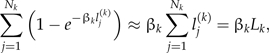where L_k is the total length of all the lineages in interval k.

The posterior distribution of β_k can now be written as

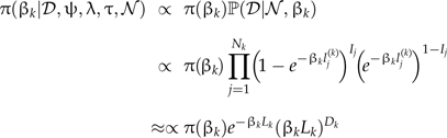and so we can use conjugate gamma prior distributions, β_k∼G(a,b). The posterior distributions are then also gamma distributions

When a and b are small the posterior means of the sampling rates are again close to their intuitive value:

(9)

References

- Alroy J. Chicago. University of Chicago; 1994. Quantitative mammalian biochronology and biogeography of North America [PhD thesis] (IL) [Google Scholar]
- Andrews P, Harrison T, Delson E, Bernor RL, Martin L. In: Distribution and biochronology of European and Southwest Asian Miocene catarrhines. The evolution of western Eurasian Neogene mammal faunas. Bernor RL, Fahlbusch V, Mittmann H-W, editors. New York: Columbia University Press; 1996. pp. 168–207. [Google Scholar]
- Andrews P, Kelley J. Middle Miocene dispersals of apes. Folia Primatol. 2007;78:328–343. doi: 10.1159/000105148. [DOI] [PubMed] [Google Scholar]
- Azzalini A. Padova, Italy: Università di Padova; 2010. R package sn: the skew-normal and skew- tdistributions. Version 0.4-15. [Google Scholar]
- Azzalini A, Genton M. Robust likelihood methods based on the skew-t and related distributions. Int. Stat. Rev. 2007;76:106–129. [Google Scholar]
- Barnett R, Barnes I, Phillips MJ, Martin LD, Harington CR, Leonard JA, Cooper A. Evolution of the extinct Sabretooths and the American cheetah-like cat. Curr. Biol. 2005;15:R589–R590. doi: 10.1016/j.cub.2005.07.052. [DOI] [PubMed] [Google Scholar]
- Beaumont MA, Zhang W, Balding DJ. Approximate Bayesian computation in population genetics. Genetics. 2002;162:2025–2035. doi: 10.1093/genetics/162.4.2025. [DOI] [PMC free article] [PubMed] [Google Scholar]
- Benton MJ, Donoghue PCJ. Paleontological evidence to date the tree of life. Mol. Biol. Evol. 2007;24:26–53. doi: 10.1093/molbev/msl150. [DOI] [PubMed] [Google Scholar]
- Brooks SP. Markov chain Monte Carlo method and its applications. Statistician. 1998;47:69–100. [Google Scholar]
- Brudno M, Chapman M, Göttgens B, Batzoglou S, Morgenstern B. Fast and sensitive multiple alignment of large genomic sequences. BMC Bioinformatics. 2003;4:66. doi: 10.1186/1471-2105-4-66. [DOI] [PMC free article] [PubMed] [Google Scholar]
- Brunet M, Guy F, Pilbeam D, Mackaye HT, Likius A, Ahounta D, Beauvilain A, Blondel C, Bocherens H, Boisserie J-R, De Bonis L, Coppens Y, Dejax J, Denys C, Duringer P, Eisenmann V, Fanone G, Fronty P, Geraads D, Lehmann T, Lihoreau F, Louchart A, Mahamat A, Merceron G, Mouchelin G, Otero O, Campomanes PP, de León MP, Rage J-C, Sapanet M, Schuster M, Sudre J, Tassy P, Valentin X, Vignaud P, Viriot L, Zazzo A, Zollikofer C. A new hominid from the Upper Miocene of Chad, Central Africa. Nature. 2002;418:145–151. doi: 10.1038/nature00879. [DOI] [PubMed] [Google Scholar]
- Chaimanee Y, Jolly D, Benammi M. Tafforeau p., Duzer D., Moussa I., Jaeger J.-J. A Middle Miocene hominoid from Thailand and orangutan origins. Nature. 2003;422:61–65. doi: 10.1038/nature01449. [DOI] [PubMed] [Google Scholar]
- Chatterjee H, Ho S, Barnes I, Groves C. Estimating the phylogeny and divergence times of primates using a supermatrix approach. BMC Evol. Biol. 2009;9:259. doi: 10.1186/1471-2148-9-259. [DOI] [PMC free article] [PubMed] [Google Scholar]
- Cooper GM, Stone EA, Asimenos G, Green E, Batzoglou S, Sidow A. Distribution and intensity of constraint in mammalian genomic sequence. Genome Res. 2005;15:901–913. doi: 10.1101/gr.3577405. [DOI] [PMC free article] [PubMed] [Google Scholar]
- Drummond AJ, Ho SYW, Phillips MJ, Rambaut A. Relaxed phylogenetics and dating with confidence. PLoS Biol. 2006:4–e88. doi: 10.1371/journal.pbio.0040088. [DOI] [PMC free article] [PubMed] [Google Scholar]
- Foote M, Hunter JP, Janis CM, Sepkoski JJ., Jr. Evolutionary and preservational constraints on origins of biological groups: divergence times of eutherian mammals. Science. 1999;283:1310–1314. doi: 10.1126/science.283.5406.1310. [DOI] [PubMed] [Google Scholar]
- Goodman M, Porter CA, Czelusniak J, Page SL, Schneider H, Shoshani J, Gunnell G, Groves CP. Toward a phylogenetic classification of primates based on DNA evidence complemented by fossil evidence. Mol. Phylogenet. Evol. 1998;9:585–598. doi: 10.1006/mpev.1998.0495. [DOI] [PubMed] [Google Scholar]
- Graur D, Martin W. Reading the entrails of chickens: molecular timescales of evolution and the illusion of precision. Trends Genet. 2004;20:80–86. doi: 10.1016/j.tig.2003.12.003. [DOI] [PubMed] [Google Scholar]
- Groves CP. In: Order primates. Mammal species of the world: a taxonomic and geographic reference. 3rd ed. Wilson DE, Reeder DM, editors. Volume 1. Baltimore (MD): John Hopkins University Press; 2005. pp. 111–184. [Google Scholar]
- Haile-Selassie Y, Suwa G, White T. Late Miocene teeth from the Middle Awash, Ethiopia, and early hominid dental evolution. Nature. 2004;303:1503–1505. doi: 10.1126/science.1092978. [DOI] [PubMed] [Google Scholar]
- Harris TE. Berlin (Germany): Springer. 1963. The theory of branching processes. [Google Scholar]
- Harrison T. Apes among the tangled branches of human origins. Science. 2010;327:532–534. doi: 10.1126/science.1184703. [DOI] [PubMed] [Google Scholar]
- Hasegawa M, Kishino H, Yano T. Dating the human-ape splitting by a molecular clock of mitrochondrial DNA.J. Mol. Evol. 1985;22:160–174. doi: 10.1007/BF02101694. [DOI] [PubMed] [Google Scholar]
- Hedges SB, Kumar S. Precision of molecular time estimates. Trends Genet. 2004;20:242–247. doi: 10.1016/j.tig.2004.03.004. [DOI] [PubMed] [Google Scholar]
- Inoue J, Donoghue PCJ, Yang Z. The impact of the representation of fossil calibrations on Bayesian estimation of species divergence times. Syst. Biol. 2010;59:74–89. doi: 10.1093/sysbio/syp078. [DOI] [PubMed] [Google Scholar]
- International Commission on Stratigraphy. IUGS ratified ICS recommendation on redefinition of Pleistocene and formal definition of base of Quaternary; 23-07-2009. Technical Report. International Commission on Stratigraphy. 2009 Available from: http://www.stratigraphy.org/ [Google Scholar]
- Jukes T, Cantor C. In: Evolution of protein molecules. Mammalian protein metabolism. Munro H, editor. New York: Academic Press; 1969. pp. 21–123. [Google Scholar]
- Kappelman J, Rasmussen DT, Sanders WJ, Feseha M, Bown T, Copeland P, Crabaugh J, Fleagle J, Glantz M, Gordon A, Jacobs B, Maga M, Muldoon K, Pan A, Pyne L, Richmond B, Ryan T, Seiffert ER, Sen S, Todd L, Wiemann MC, Winkler A. Oligocene mammals from Ethiopia and faunal exchange between Afro-Arabia and Eurasia. Nature. 2003;426:549–552. doi: 10.1038/nature02102. [DOI] [PubMed] [Google Scholar]
- Kay RF, Fleagle JG, Mitchell TRT, Colbert M, Bown T, Powers DW. The anatomy of Dolichocebus gaimanensis, a stem platyrrhine monkey from Argentina. J. Hum. Evol. 2008;54:323–382. doi: 10.1016/j.jhevol.2007.09.002. [DOI] [PubMed] [Google Scholar]
- Kendall DG. On the generalized birth-and-death process. Ann. Math. Stat. 1948;19:1–15. [Google Scholar]
- Kent WJ. BLAT—the BLAST-like alignment tool. Genome Res. 2002;12:656–664. doi: 10.1101/gr.229202. [DOI] [PMC free article] [PubMed] [Google Scholar]
- Kontoyiannis I, Harremoes P, Johnson O. Entropy and the law of small numbers. IEEE T. Inform. Theory. 2005;51:466–472. [Google Scholar]
- Krause DW, Maas MC. The biogeographic origins of late Paleocene-early Eocene mammalian immigrants to the western interior of North America. Geol. Soc. Am. (Special Papers) 1990;243:71–105. [Google Scholar]
- Leakey MG, Feibel CS, McDougall I, Ward C, Walker AC. New specimens and confirmation of an early age for Australopithecus anamensis. Nature. 1998;393:62–66. doi: 10.1038/29972. [DOI] [PubMed] [Google Scholar]
- Marjoram P, Molitor J, Plagnol V, Tavaré S. Markov chain Monte Carlo without likelihoods. Proc. Natl. Acad. Sci. USA. 2003;100:15324–15328. doi: 10.1073/pnas.0306899100. [DOI] [PMC free article] [PubMed] [Google Scholar]
- Martin RD. Primate origins: plugging the gaps. Nature. 1993;363:233–234. doi: 10.1038/363223a0. [DOI] [PubMed] [Google Scholar]
- Martin RD, Soligo C, Tavaré S. Primate origins: implications of a Cretaceous ancestry. Folia Primatol. 2007;78:277–296. doi: 10.1159/000105145. [DOI] [PubMed] [Google Scholar]
- McGowan AJ, Smith AB. Are global Phanerozoic diversity curves truly global? A study of the relationship between regional rock records and global Phanerozoic marine diversity. Paleobiology. 2008;34:80–103. [Google Scholar]
- Miller ER, Benefit BR, McCrossin ML, Plavcan JM, Leakey MG, El-Barkooky AN, Hamdan MA, Abdel Gawad MK, Hassan SM, Simons EL. Systematics of early and middle Miocene Old World monkeys. J. Hum. Evol. 2009;57:195–211. doi: 10.1016/j.jhevol.2009.06.006. [DOI] [PubMed] [Google Scholar]
- Miller ER, Gunnell GF, Martin RD. Deep time and the search for anthropoid origins. Yrbk. phys. Anthropol. 2005;48:60–95. doi: 10.1002/ajpa.20352. [DOI] [PubMed] [Google Scholar]
- Ni X, Wang Y, Hu Y, Li C. A euprimate skull from the early Eocene of China. Nature. 2004;427:65–68. doi: 10.1038/nature02126. [DOI] [PubMed] [Google Scholar]
- Paul CRC. The fidelity of the fossil record: the improbability of preservation. Palaeontology. 2009;52:485–489. [Google Scholar]
- Peters SE, Foote M. Biodiversity in the Phanerozoic: a reinterpretation. Paleobiology. 2001;27:583–601. [Google Scholar]
- Rannala B, Yang Z. Inferring speciation times under an episodic molecular clock. Syst. Biol. 2007;56:453–466. doi: 10.1080/10635150701420643. [DOI] [PubMed] [Google Scholar]
- Raup DM. Species diversity in the Phanerozoic: an interpretation. Paleobiology. 1976;2:289–297. [Google Scholar]
- Ray DA, Xing J, Hedges DJ, Hall MA, Laborde ME, Anders BA, White BR, Stoilova N, Fowlkes JD, Landry KE, Chemnick LG, Ryder OA, Batzer MA. Alu insertion loci and platyrrhine primate phylogeny. Mol. Phylogenet. Evol. 2005;35:117–126. doi: 10.1016/j.ympev.2004.10.023. [DOI] [PubMed] [Google Scholar]
- Ripley BD. Stochastic simulation. New York: Wiley; 1987. [Google Scholar]
- Seiffert E. Evolution and extinction of Afro-Arabian primates near the Eocene-Oligocene boundary. Folia Primatol. 2007;78:314–327. doi: 10.1159/000105147. [DOI] [PubMed] [Google Scholar]
- Senut B, Pickford M, Gommery D, Mein P, Cheboi K, Coppens Y. First hominid from the Miocene (Lukeino Formation, Kenya). C R Acad. Sci. IIA Earth Planet. Sci. 2001;332:137–144. [Google Scholar]
- Sisson SA, Fan Y, Tanaka MM. Sequential Monte Carlo without likelihoods. Proc. Natl. Acad. Sci. USA. 2007;104:1760–1765. doi: 10.1073/pnas.0607208104. [DOI] [PMC free article] [PubMed] [Google Scholar]
- Smit AFA, Hubley R, Green P. 1996–2004. RepeatMasker Open-3.0. Available from: http://www.repeatmasker.org. [Google Scholar]
- Smith AB, Peterson KJ. Molecular clocks and the fossil record. Annu. Rev. Earth Planet Sci. 2002;30:65–88. [Google Scholar]
- Smith T, Rose KD, Gingerich PD. Rapid Asia-Europe-North America geographic dispersal of earliest Eocene primate Teilhardina during the Paleocene-Eocene Thermal Maximum. Proc. Nat. Acad. Sci. USA. 2006;103:11223–11227. doi: 10.1073/pnas.0511296103. [DOI] [PMC free article] [PubMed] [Google Scholar]
- Soligo C. Invading Europe: did climate or geography trigger early Eocene primate dispersals? Folia Primatol. 2007;78:297–313. doi: 10.1159/000105146. [DOI] [PubMed] [Google Scholar]
- Soligo C, Martin RD. Adaptive origins of primates revisited. J. Hum. Evol. 2006;50:414–430. doi: 10.1016/j.jhevol.2005.11.001. [DOI] [PubMed] [Google Scholar]
- Soligo C, Will O, Tavaré S, Marshall CR, Martin RD. New light on the dates of primate origins and divergence. In: Ravosa MJ, Dagosto M, editors. Primate origins: adaptations and evolution. New York: Springer; 2007. pp. 29–49. [Google Scholar]
- Steiper ME, Young NM. Primate molecular divergence dates. Mol. Phylogenet. Evol. 2006;41:384–394. doi: 10.1016/j.ympev.2006.05.021. [DOI] [PubMed] [Google Scholar]
- Steiper ME, Young NM. Timing primate evolution: lessons from the discordance between molecular and paleontological estimates. Evol. Anthropol. 2008;17:179–188. [Google Scholar]
- Steiper ME, Young NM. In: Primates Timetree of life. Hedges SB, Kumar S, editors. Oxford: Oxford University Press; 2009. pp. 482–486. [Google Scholar]
- Steiper ME, Young NM, Sukarna TY. Genomic data support the hominoid slowdown and an early Oligocene estimate for the hominoid-cercopithecoid divergence. Proc. Natl. Acad. Sci. USA. 2004;101:17021–17026. doi: 10.1073/pnas.0407270101. [DOI] [PMC free article] [PubMed] [Google Scholar]
- Tavaré S, Marshall CR, Will O, Soligo C, Martin RD. Using the fossil record to estimate the age of the last common ancestor of extant primates. Nature. 2002;416:726–729. doi: 10.1038/416726a. [DOI] [PubMed] [Google Scholar]
- Thorne J, Kishino H, Painter I. Estimating the rate of evolution of the rate of molecular evolution. Mol. Biol. Evol. 1998;15:1647–1657. doi: 10.1093/oxfordjournals.molbev.a025892. [DOI] [PubMed] [Google Scholar]
- Tierney L. Markov chains for exploring posterior distributions. Ann. Stat. 1994;22:1701–1762. [Google Scholar]
- Wang QF, Prabhakar S, Chanan S, Cheng JF, Rubin EM, Boffelli D. Detection of weakly conserved ancestral mammalian regulatory sequences by primate comparisons. Genome Biol. 2007;8:R1. doi: 10.1186/gb-2007-8-1-r1. [DOI] [PMC free article] [PubMed] [Google Scholar]
- Wang SC, Dobson P. Estimating the diversity of dinosaurs. Proc. Natl. Acad. Sci. USA. 2006;103:13601–13605. doi: 10.1073/pnas.0606028103. [DOI] [PMC free article] [PubMed] [Google Scholar]
- Wilkinson RD. Bayesian inference of primate divergence times [PhD thesis] Cambridge, UK: University of Cambridge; 2007. [Google Scholar]
- Wilkinson RD, Tavaré S. Estimating primate divergence times by using conditioned birth-and-death processes. Theor. Popul. Biol. 2009;75:278–285. doi: 10.1016/j.tpb.2009.02.003. [DOI] [PubMed] [Google Scholar]
- Yang Z. Maximum likelihood phylogenetic estimation from DNA sequences with variable rates over sites: approximate methods. J. Mol. Evol. 1994;39:306–314. doi: 10.1007/BF00160154. [DOI] [PubMed] [Google Scholar]
- Yang Z. PAML 4: phylogenetic analysis by maximum likelihood. Mol. Bio. Evol. 2007;24:1586–1591. doi: 10.1093/molbev/msm088. [DOI] [PubMed] [Google Scholar]
- Yang Z, Rannala B. Bayesian estimation of species divergence times under a molecular clock using multiple fossil calibrations with soft bounds. Mol. Biol. Evol. 2006;23:212–226. doi: 10.1093/molbev/msj024. [DOI] [PubMed] [Google Scholar]
Associated Data
This section collects any data citations, data availability statements, or supplementary materials included in this article.