Initialization Parameter Sweep in ATHENA: Optimizing Neural Networks for Detecting Gene-Gene Interactions in the Presence of Small Main Effects

Abstract

Recent advances in genotyping technology have led to the generation of an enormous quantity of genetic data. Traditional methods of statistical analysis have proved insufficient in extracting all of the information about the genetic components of common, complex human diseases. A contributing factor to the problem of analysis is that amongst the small main effects of each single gene on disease susceptibility, there are non-linear, gene-gene interactions that can be difficult for traditional, parametric analyses to detect. In addition, exhaustively searching all multi-locus combinations has proved computationally impractical. Novel strategies for analysis have been developed to address these issues. The Analysis Tool for Heritable and Environmental Network Associations (ATHENA) is an analytical tool that incorporates grammatical evolution neural networks (GENN) to detect interactions among genetic factors. Initial parameters define how the evolutionary process will be implemented. This research addresses how different parameter settings affect detection of disease models involving interactions. In the current study, we iterate over multiple parameter values to determine which combinations appear optimal for detecting interactions in simulated data for multiple genetic models. Our results indicate that the factors that have the greatest influence on detection are: input variable encoding, population size, and parallel computation.

1. INTRODUCTION

One of the greatest challenges in the field of human genetics is the identification of genetic and environmental factors which confer susceptibility to common, complex diseases. Traditionally, the focus of association analysis has been on one or a few possible genes that exhibit large main effects. However, recent studies of complex disease such as hypertension [7] and breast cancer [16] have shown that many disease susceptibility gene effects rely on interactions with other genetic and environmental factors. We are only beginning to understand how to identify these non-linear interaction effects [8] [3]. In addition to the complexity of these non-linear interactions, there has been a surge of rapidly advancing genotyping technology and an explosion of genetic information availability. Exhaustively searching all multi-locus combinations has proven computationally impractical, and novel strategies for analysis have been developed in order to address these issues.

Our lab is developing the Analysis Tool for Heritable and Environmental Network Associations (ATHENA), a multi-functional analytical tool designed to perform the three main functions essential to determining the genetic architecture of complex diseases: performing variable selection from categorical or continuous independent variables, modeling main and interaction effects that best predict categorical or continuous outcome data, and interpreting the significant models for use in further biomedical research (Figure 1). ATHENA is unique in its ability to integrate multiple types of information relevant to a phenotype (examples: single nucleotide polymorphisms (SNPs), microarray, proteomics, and clinical data) that can be combined and used for a single analysis. In addition, ATHENA incorporates Biofilter [2], which makes use of publicly available biological domain knowledge, in order to filter out statistical noise in favor of signals that have true biological relevance. Several different strategies that are effective in modeling genetic susceptibility factors will be available in the software package (examples: grammatical evolution neural networks, regression and classification trees, support vector machines) [9]. The goal of ATHENA is to perform sophisticated analysis of genetic, genomic, and other biological data for use in a complex association analysis. In this study, we focus specifically on optimizing the initialization parameter settings in the grammatical evolution neural networks (GENN) analytical algorithm that operates within ATHENA.

Figure 1.

Schematic of ATHENA: Analysis Tool for Heritable and Environmental Network Associations.

Neural networks (NN) were originally designed to model the neuron in the brain. NN take advantage of the brain's ability to problem solve by processing data in parallel, whereas computers traditionally operate sequentially. Put simply, neural networks are a collection of simple analog processors in parallel, which analyze an input pattern in order to generate an output signal. Each input node represents a variable (such as SNP genotype) that is multiplied by a weight, processed by a function, and then gives an output [18]. The output can be continuous or discrete. Conventionally, neural networks are trained for pattern recognition using a gradient descent algorithm such as back-propagation [1]. This involves predefining the architecture (nodes and variables) of the network and then adjusting the weights to minimize error in classification; for example, whether or not an individual has a disease based on their genotypes at certain SNPs. Alternatively, GENN uses evolutionary computation (EC) to optimize neural networks and detect genetic models associated with a particular phenotype. This is not a novel concept; EC has been used to evolve NN in other fields of study such as aircraft simulation, robot path planning, and many more [19]. However, one of the benefits of EC is that it does not require a priori variable selection or architecture definition, rather it allows the user to optimize weight, inputs, and architecture simultaneously [6]. The underlying model for each disease is different, and widening the search space to include all possible networks is optimal. GENN can outperform back-propagation and random search strategies in finding gene-gene interactions in simulated data sets [12].

However, when using the evolutionary algorithm GENN, it remains unclear how variation in initial parameter settings influences the ability of GENN to detect specific genetic models. In this study, we examined how specific combinations of GENN parameters affected the ability of ATHENA to detect a realistic 2-locus model with both an interaction effect and smaller main effects. To avoid confusion, we will be referring to the analytic algorithm that is being optimized as GENN and the software that allows us to run the algorithm as ATHENA.

2. METHODS

2.1 GENN

GENN is a variation on Genetic Programming of Neural Networks (GPNN) [17]. The main difference being that in GPNN, evolutionary operators such as cross-over and mutation act directly on the neural network, whereas in GENN, evolution occurs at the level of the binary string which is later translated into a neural network using a set of rules or grammars. The details of grammatical evolution can be found in [12] and [14]. In Figure 2, the left side represents the central dogma of molecular biology compared to the right side which represents GENN. This figure shows the steps of transcription and translation to integers and neural networks, then selection occurring at the phenotype level using fitness functions. GENN evolution allows for a more computationally efficient analysis because evolution takes place on a simple binary string rather than an entire neural network and thus creates more genetic diversity. This efficiency has been demonstrated using simulated data sets [10] [12] .

Figure 2.

Central dogma (left) of molecular biology and evolution by natural selection to GENN (right).

The first step of the GENN algorithm is to initialize a set of parameters that specify the details of the evolutionary process in the configuration file. Next, each dataset is divided into 5 equal parts for 5-fold cross validation (4/5 for training and 1/5 for testing) to prevent over-fitting of the data. Training begins by generating a population of random binary strings initialized to be functional neural networks using sensible initialization [12]. Each NN in the population is then evaluated on the training data, and its fitness is recorded. The best solutions are selected for crossover and reproduction, and a new population is created. The steps are repeated for a pre-defined number of generations. For each generation, the newly “evolved” population is tested on the training data with an optimal solution being selected. The overall best solution across generations is run on 1/5 of the data left out for testing, and prediction error (discrete outcome) or mean-squared error (continuous outcome) is recorded. The entire process is repeated 5 times, each time using different 4/5 of data for training and 1/5 for testing. The best model per dataset is the model that was chosen the most over the 5 cross-validations.

2.2 Data Simulation

When developing and evaluating novel computational and statistical methods, it is important to simulate data with characteristics of real genetic data. In order to address this need, we created genomeSIMLA. This software has previously been described in detail [4] [4]. The simulated data sets are used to test the method's robustness to specific complexities such as nonlinear loci interactions that contribute to a measurable phenotype. In this study, we used simulated data to test the effect of specific GENN evolutionary parameters on ability of the serial and parallel version of ATHENA to detect gene-gene interactions in the presence of small main effects.

For each model, we created 100 data sets: 1000 individuals per data set, each individual with genotypes for 10, 50 or 100 SNPs, and a quantitative trait outcome. Individuals were randomly selected from a normally distributed population with a mean close to 0 and a homoscedastic standard deviation of 1. For all models, two SNPs were functional loci that contributed to a specific proportion of variation in the outcome, also referred to as heritability. The functional SNPs had a main effect heritability of 0.01, an interaction effect heritability of 0.05, and a minor allele frequency of 0.25. These simulated attributes are similar to what is likely to be found in real genome-wide data. We simulated both additive and dominant effects in our genetic models. In an additive model, the probability of affecting the quantitative trait increases with each additional minor allele. (AABB < AaBb < aabb). In a dominant model, only one minor allele at a particular locus is necessary to confer increased probability (AABB < AaBB < aabb = aaBb = AaBb). The mean for each multilocus genotype can be found in Table 1 and Table 2 (a and b are the minor alleles). The genotype frequencies were calculated under the assumption of Hardy-Weinberg Equilibrium.

Table 1.

Additive Effect Genotype Penetrance Table (Genotype Frequency in Parentheses)

	AA (0.5625)	Aa (0.375)	aa (0.0625)
BB (0.5625)	0	0.22	0.44
Bb (0.375)	0.22	1.18	2.14
bb (0.0625)	0.44	2.14	3.84

Table 2.

Dominant Effect Genotype Penetrance Table (Genotype Frequency in Parentheses)

	AA (0.5625)	Aa (0.375)	aa (0.0625)
BB (0.5625)	0	0.25	0.25
Bb (0.375)	0.25	1.82	1.82
bb (0.0625)	0.25	1.82	1.82

We recognize that even 100 SNPs per individual is a much smaller number of input variables than would be normally be seen in genome wide association studies (GWAS), which is most commonly around 500,000 to 1,000,000 SNPs. However, when testing new methods, it is imperative to save time and computational resources by starting with small datasets, discovering what changes in the program result in improvements, and implementing those changes in larger data sets. Our smaller number of inputs allowed us to focus on optimization and reducing variability that could arise in more complex data sets. In the future, ATHENA will continue to be validated in larger simulated data sets and with actual genetic data.

2.3 Data Analysis

We divided our experiments into two separate analyses: Analysis I tested four simulation models on 48 different parameter combinations, while Analysis II specifically tested the effect of different variable encoding options using two simulation models and 24 parameter combinations (Table 3). An explanation of all of the parameters is found in Section 2.3. Each analysis was completed on both the serial and parallel versions of ATHENA. For every run, all evolutionary parameters not being iterated over were held constant: 100 generations, cross-over rate of 0.9, and a mutation rate of 0.01. We calculated how many times out of the 100 data sets both functional loci were identified as the best model for each parameter combination. The number of data sets where this occurred will be referred to as “detection power.” We compared the detection power for each parameter combination to see if any specific combination(s) performed better than others.

Table 3.

Experimental Design: Simulation Model Descriptions and Parameter Iteration Values (A = Additive, D = Dominant)

		Analysis I	Analysis II
Simulation Models	SNPs / Genetic Effect	10 / A	100 / A
		10 / D
		50 / A	100 / D
		100 / A
Parameter Iterations	PopSize	50, 200, 400, 600, 800, 1000	50, 200, 400, 600, 800, 1000
	MaxDepth	7, 15	7
	GrammarFile	Add, All	Add, All
	DummyEncode	True, False	Re-coded: Linear, Quadratic
	Total Parameters per Model	48	24

We also compared serial and parallel versions of ATHENA because sequentially, the GENN algorithm is effective for searching highly nonlinear, multidimensional search spaces, but it is still susceptible to stalling on local minima as the best solution. Parallel ATHENA attempts to address this problem by running the GENN algorithm using isolated demes (or sub-populations) of solutions on a predetermined number of processors. A periodic exchange or “migration” of best solutions between demes occurs a set number of times during each run. This exchange increases diversity among the solutions in the different populations and decreases stalling at local minima [11]. We wanted to determine if there was a threshold at which dividing the population size into smaller subpopulations was no longer beneficial. Also, we wanted to complete a thorough analysis of the difference in computation time between the two versions.

2.3 Parameter Descriptions

For this experiment, we iterated over specific values for four parameters which affect the evolutionary process of GENN (see Table 3). Below, we describe these parameters in detail.

2.3.1 PopSize

Population size is the number of random solutions generated at the beginning of the evolutionary process. The solutions are binary strings generated to be functional neural networks using sensible initialization [12]. This population size remains constant across all generations.

It is important to note that parallel ATHENA divides the population size by the number of nodes indicated in the configuration file in order to create sub-populations, or demes. In this study, we ran parallel ATHENA on four nodes. Thus, each population size in parallel ATHENA was divided into 4 equal demes. For example, if we specify a population size of 200, parallel ATHENA will create four isolated demes of size 50 on each node which separately undergo evolutionary processes before migration of best solutions between demes. For this study, migration occurred four times over 100 generations. In comparison, serial ATHENA will create one population size of 200 where all evolution occurs, and there is no migration. When we are comparing serial ATHENA to parallel ATHENA, we are comparing the total population size, not deme size. We chose an array of population sizes in order to determine the smallest population size which maximizes detection power.

2.3.2 MaxDepth

This parameter only affects the process of sensible initialization whereby each of the binary strings in the initial population of solutions is primed to be a functional neural network. MaxDepth defines the maximum depth of sequential rules that are allowed in the expression tree that initializes the binary strings to be neural networks. In other words, it is the maximum number of grammar rules that each branch of the expression tree can contain. Theoretically, a larger maximum depth would confer larger, more complex neural networks in the original population. In previous experiments, 10 was used for the MaxDepth. We chose values above and below 10, specifically 7 and 15, to determine if more complex networks would affect the ability of the GENN algorithm to detect the correct susceptibility model.

2.3.3 GrammarFile

The grammar file is the text file that specifies the details of the grammar being used when translating the binary strings into neural networks. We chose to iterate through an “add-only” grammar and an “all” grammar. The “add-only” option creates neural networks with activation functions that only use addition, while the “all” option allows activation functions to be addition, subtraction, multiplication, and protected division.

2.3.4 DummyEncode

The dummy-encoding method used in GENN is a method of genotype representation developed by Jurg Ott [15] specifically for genetic data analysis using neural networks. This method creates two new “dummy” variables for each SNP genotype: one to encode for a linear, or allelic effect, and one to encode for a non-linear, or quadratic effect (Table 4). The basis of dummy-encoding is to allow for the representation of genotypic effects that corresponds to not only additive (linear encoding), but also dominant or recessive patterns of inheritance (quadratic encoding). The allelic, or additive, effect is represented by the dummy variable that codes genotypes as −1, 0, 1, a single unit increase of one with each additional minor allele. The genotypic, or quadratic, effect represents the genotypes as −1, 2, −1, distinguishing heterozygotes from homozygotes. If dummy encoding is not used, the SNPs are coded as 0, 1, 2, notably also an additive representation.

Table 4.

Genotype-Encoding (DE = dummy-encoding)

Genotype	No DE	DE
		Linear	Quadratic
AA	0	−1	−1
Aa	1	0	2
aa	2	1	−1

For Analysis I, we either turned dummy-encoding on (TRUE) or off (FALSE), to determine if the different methods of genotype representation affect detection power. For Analysis II, we recoded the genotypes as the either the linear variable (−1, 0, 1) or the quadratic variable (−1, 2, −1) and then compared the detection power of the separate dummy variables on both an additive and a dominant model.

An example ATHENA configuration file and the grammar rule files can be found here under the title “Related Links”: http://chgr.mc.vanderbilt.edu/ritchielab/method.php?method=athena

3. RESULTS

3.1 Parameter Analysis

In Analysis I, we iterated over different values for four different GENN evolutionary parameters for a total of 48 parameter combinations (see Table 3, Analysis I). We ran both the serial and parallel version of the ATHENA software for each of these combinations on four different simulation models in order to determine which factors maximized detection power. Figure 3 and Figure 4 show the results for serial ATHENA and parallel ATHENA, respectively.

Figure 3.

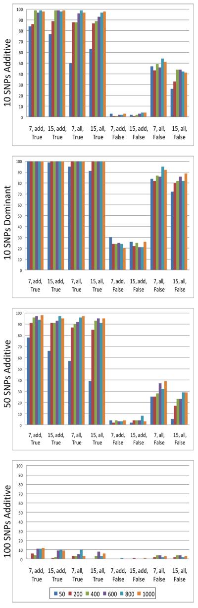
Serial ATHENA parameter combination results. Different color bars represent different values for PopSize (as indicated in figure legend). At each position, the x-axis values represent MaxDepth, GrammarFile, and DummyEncode. Detection power values are shown on the y-axis.

Figure 4.

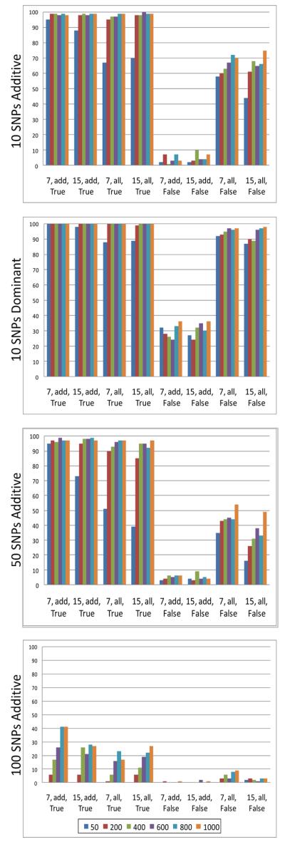
Parallel ATHENA parameter combination results. Different color bars represent different values for PopSize (as indicated in figure legend). At each position, the x-axis values represent MaxDepth, GrammarFile, and DummyEncode. Detection power values are shown on the y-axis.

Because we were interested in determining whether dividing the population size into very small demes could have a negative impact on the detection power of parallel ATHENA, we found it notable that even at the smallest population size (50), parallel ATHENA performed as well as serial ATHENA. In fact, the detection power was greater in all of the additive models.

For both the serial and parallel versions of ATHENA, detection power increased with population size. The highest detection power was seen when the SNP genotypes were dummy-encoded. For each simulation model, the lowest detection power was observed when SNPs were not dummy-encoded and “add-only” grammar was used. Interestingly, there appeared to be a substantial increase in detection power associated with not dummy-encoding while using “all” grammar, most noticeable in the dominant model. The different values for maximum depth did not appear to have a consistent affect on detection power in any of the simulation models.

3.2 Dummy-Encoding Analysis

In Analysis II, we compared the linear and quadratic components of dummy-encoding (as described in Table 4) on both an additive and dominant 100-SNP simulation model in order to determine if either component conferred an increase in detection power that was specific to genetic effect. In Figure 5, dummy-encoding (DE) represents using both linear and quadratic effects such that there are two new variables representing each single independent variable (same as DE=TRUE in Analysis I). In contrast, the linear and quadratic components are single variable replacements for each independent variable. In essence, the DE set consists of 200 independent variables to choose from where the linear and quadratic encoding sets have only 100 independent variables.

Figure 5.

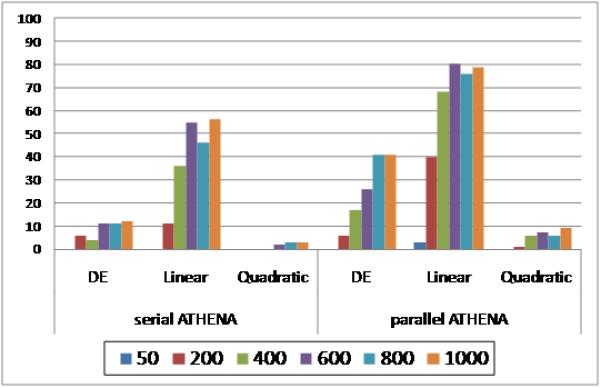
A comparison of dummy-encoding with its linear and quadratic components. Here we are showing the detection power (y-axis) for the additive 100 SNP simulation models. Different color bars represent different population sizes. (MaxDepth = 7 and GrammarFile = add)

Figure 5 shows the results for the additive model comparing dummy-encoding from Analysis I (DE), the linear dummy variable, and the quadratic dummy variable. We are displaying the “add-only” grammar results because it was associated with the highest detection power when dummy-encoding was used.

Our results show that encoding SNP genotypes using the linear dummy variable resulted in greater detection power than both the quadratic dummy variable and dummy-encoding. We saw the same trend for the analysis of the dominant 100 SNP model. There did appear to be a slight increase in detection power in the dominant effect model over the additive effect model when the dummy variables were quadratic (data not shown), however, the linear dummy variable conferred the greatest detection power for both effect models.

3.3 Computation Time

Computation time is an important limitation in analytic software tools. In this study, some parameter combinations had striking increases in computation time without resulting in an increase in detection power. The factors that contributed the most to run-time were ATHENA version (serial or parallel), PopSize, and MaxDepth. GrammarFile, DummyEncoding and SNP counts had no consistent effect on computation time. Table 5 compares each version of ATHENA, population sizes, and maximum depth for each 50 SNP additive model from Analysis I to illustrate the effects each factor has on detection power and run time. These calculations are based on the computation time which includes both training and testing.

Table 5.

Detection Power and Computation Time for 50 SNP additive model. (GrammarFile = add, DummyEncode = True)

	PopSize	MaxDepth	Detection Power	Time (hr:min)
Serial ATHENA	50	7	78	2:14
		15	66	4:35
	1000	7	98	48:58
		15	95	95:34
Parallel ATHENA	50	7	95	0:31
		15	73	1:17
	1000	7	97	11:36
		15	97	27:19

Using the values from Table 5, parallel ATHENA computed on average 4 times faster than serial ATHENA, and, at the smaller population size, also resulted in a considerable increase in detection power. Increasing the population size from 50 to 1000 resulted in approximately a 20 fold increase in run time and better detection power, most notably in serial ATHENA. Interestingly, increasing the maximum depth from 7 to 15 more than doubled the run time but did not result in a substantial increase in detection power. These trends were seen for all simulation models.

4. DISCUSSION

For this study, we performed two analyses. The first was a broader analysis comparing the effect of specific GENN evolutionary parameter combinations on the ability of both the serial and parallel versions of ATHENA to detect gene-gene interactions with small main effects. The second analysis was to investigate the effects of dummy encoding components on detection power.

In Analysis I, the only parameter that did not appear to have a consistent impact on detection power, but increased computation time, was maximum depth. As described in Section 2.3.2, the maximum depth is the maximum number of grammar rules that are allowed in the expression tree that the GENN algorithm uses during sensible initialization to guarantee that all binary strings will be functional neural networks. An increase in maximum depth, therefore, could result in more complex neural networks in the initial population. Because the simulated susceptibility model is very simple (2 locus with an interaction effect and smaller main effects), a maximum depth of 7 was sufficient to generate neural networks with properties that allowed them to be similar to the correct solution. If we had simulated a more complex model, for example, with 5 interacting loci, each with varying main effects, we may have seen a benefit associated with using a larger maximum depth. Further optimization analyses will have to be run to test this hypothesis.

More densely surveying the solution space is inherently beneficial to genetic programming. Therefore, we anticipated the observed increase in detection power associated with increasing the population size for GENN. Larger population sizes also increased computation time. To enhance efficiency without sacrificing accuracy, we determined the smallest population size at which we could achieve maximum detection power. This threshold was different for the different versions of ATHENA and for different simulation models (Figure 3 and Figure 4). Increasing the number of SNPs, or input variables, to 100 made it difficult for either version to achieve reasonable detection power; however, running the algorithm in parallel conferred a boost in detection power.

We were also interested in determining if there was a population size at which division into smaller isolated demes was no longer beneficial. Even at the smallest population size of 50, where the deme size would have been very small (approximately 12), parallel ATHENA still achieved greater detection power. This serves as additional evidence for the benefit of the “island model” and suggests that migration of best solutions between demes prevents stalling on local minima in the fitness landscape [11].

We also saw what appeared to be an interaction between “add-only” grammar and dummy-encoding that resulted in greater detection power. These grammar rules only allow addition activation functions in the NN, and this suggest these parameters allow more efficient evolution to find the correct solution. The considerable increase in detection power seen in the 10 SNP dominant model with “all” grammar and no dummy-encoding suggests that genetic effect could be a factor.

The large increase in detection power associated with dummy-encoding was especially interesting for the additive effect simulation models, because when dummy-encoding was not used, the SNPs were still represented in an additive fashion (0, 1, 2), and it follows logic that either additive encoding should have been able to detect the additive effect equally as well. Furthermore, dummy-encoding creates a new, non-linear variable. This doubles the number of input variables to be analyzed by the neural network. It would be reasonable to assume that increasing the number of inputs or variables would decrease the ability of the neural network to perform accurate variable selection. However, these speculations were not supported by our results. This suggests that there is something inherent about the dummy-variable encodings that conferred in increase in detection power, and led us to complete Analysis II.

In Analysis II, we decomposed dummy-encoding into its separate components to determine if one of them was individually responsible for the increase in detection power observed when dummy-encoding was used. We re-coded the SNPs as either linear or quadratic dummy variables (as shown in Table 4) for both additive and dominant effect genetic models. We chose to use 100 SNPs because the detection power was lowest for 100 SNPs in our first analysis, and therefore, more likely to discern an increase in detection power. We observed a considerable increase in detection power when the SNP genotypes were encoded as the linear dummy variable (−1, 0, 1) for both the additive (see Figure 5) and dominant effect models. This increase in detection power was probably directly associated with reducing the number of input variables by half. The benefit associated with the linear dummy variable itself, however, is more complex to analyze. There could be an advantage due to the use of zeroes and ones, the use of a negative encoding for one of the genotypes, or something more relevant to how neural networks recognize patterns in data. More analyses will have to be done to determine more definitively how encoding input variables affects the ability of GENN to detect susceptibility models.

The immediate benefit of using parallel ATHENA to run the GENN algorithm was the significant decrease in computation time. Running the parameter sweep in serial took approximately four times longer to run. Running the software in parallel allowed each analysis to be spread out over several processors and thus decrease computation time without losing detection power.

The broadest implication of this study was to better understand evolutionary computation and how altering the process of evolution can result in an optimized combination of parameters that allows for accurate variable selection and modeling of complex interactions among susceptibility factors. The results of this study show that optimum detection power is achieved with addition-only activation functions and when the SNP genotypes were encoded as −1, 0, 1. Future analyses will determine if our optimized parameters are robust to larger, more complicated simulated data sets and in actual genetic data. Ideally, we will discover what parameters are optimal under different conditions, and, therefore, create a software package for the public that is more user-friendly because it does not require intensive back-end alterations.

REFERENCES

- 1.Bishop CM. Neural Networks for Pattern Recognition. Oxford University Press; London: 1995. [Google Scholar]
- 2.Bush WS, Dudek SM, Ritchie MD. Biofilter: a knowledge-integration system for the multi-locus analysis of genome-wide association studies. Pac. Symp. Biocomput. 2009:368–379. [PMC free article] [PubMed] [Google Scholar]
- 3.Cordell HJ. Genome-wide association studies: Detecting gene-gene interactions that underlie human diseases. Nat Rev Genet. 2009;10:392–404. doi: 10.1038/nrg2579. [DOI] [PMC free article] [PubMed] [Google Scholar]
- 4.Dudek SM, Motsinger AA, Velez DR, Williams SM, Ritchie MD. Data Simulation Software for Whole-Genome Association and Other Studies in Human Genetics. Pac Symp BioComput. 2006:499–510. [PubMed] [Google Scholar]
- 5.Edwards TL, Bush WS, Turner SD, Dudek SM, Torstenson ES, Schmidt M, Martin E, Ritchie MD. Generating Linkage Disequilibrium Patterns in Data Simulations Using genomeSIMLA. Lecture Notes in Computer Science. 2008;4793:24–35. [Google Scholar]
- 6.Koza JR, Rice JP. Genetic generation of both the weights and architecture for a neural network. Proceeeding of the IEEE Joint Conference on Neural Networks. 1991:7–404. [Google Scholar]
- 7.Moore JH, Williams SM. New strategies for identifying gene-gene interactions in hypertension. Ann. Med. 2002;34:88–95. doi: 10.1080/07853890252953473. [DOI] [PubMed] [Google Scholar]
- 8.Moore JH. The ubiquitous nature of epistasis in determining susceptibility to common human diseases. Hum. Hered. 2003;56:73–82. doi: 10.1159/000073735. [DOI] [PubMed] [Google Scholar]
- 9.Motsinger-Reif AA, Reif DM, Fanelli TJ, Ritchie MDA. comparison of analytical methods for genetic association studies. Genet.Epidemiol. 2008;32:767–778. doi: 10.1002/gepi.20345. [DOI] [PubMed] [Google Scholar]
- 10.Motsinger-Reif AA, Dudek SM, Hahn LW, Ritchie MD. Comparison of approaches for machine-learning optimization of neural networks for detecting gene-gene interactions in genetic epidemiology. Genetic Epidemiology. 2008;32:325–340. doi: 10.1002/gepi.20307. [DOI] [PubMed] [Google Scholar]
- 11.Motsinger-Reif AA, Ritchie MD. Neural networks for genetic epidemiology: past, present, and future. BioData.Min. 2008;1:3. doi: 10.1186/1756-0381-1-3. [DOI] [PMC free article] [PubMed] [Google Scholar]
- 12.Motsinger AA, Dudek SM, Hahn LW, Ritchie MD. Comparison of neural network optimization approaches for studies of human genetics. Lecture Notes in Computer Science. 2006;3907:103–114. [Google Scholar]
- 13.O'Neill M, Ryan C. Grammatical Evolution: Evolutionary Automatic Programming in an Arbitrary Language. Kluwer Academic Publishers; Norwell, MA: 2003. [Google Scholar]
- 14.O'Neill M, Ryan C. Grammatical Evolution. IEEE Transactions on Evolutionary Computation. 2001;5:349–358. [Google Scholar]
- 15.Ott J. Neural networks and disease association studies. American Journal of Medical Genetics (Neuropsychiatric Genetics) 2001;105:60–61. [PubMed] [Google Scholar]
- 16.Ritchie MD, Hahn LW, Roodi N, Bailey LR, Dupont WD, Parl FF, Moore JH. Multifactor-dimensionality reduction reveals high-order interactions among estrogen-metabolism genes in sporadic breast cancer. Am. J. Hum. Gen. 2001;69:138–147. doi: 10.1086/321276. [DOI] [PMC free article] [PubMed] [Google Scholar]
- 17.Ritchie MD, White BC, Parker JS, Hahn LW, Moore JH. Optimization of neural network architecture using genetic programming improves detection and modeling of gene-gene interactions in studies of human diseases. BMC Bioinformatics. 2003;4:28. doi: 10.1186/1471-2105-4-28. [DOI] [PMC free article] [PubMed] [Google Scholar]
- 18.Skapura DM. Building neural networks. ACM Press; New York: 1995. [Google Scholar]
- 19.Yao Xin. Evolving Aritficial Neural Networks. Proceeedings of the IEEE. 1999:1423–1447. [Google Scholar]