Odds Ratios for Mediation Analysis for a Dichotomous Outcome

Abstract

For dichotomous outcomes, the authors discuss when the standard approaches to mediation analysis used in epidemiology and the social sciences are valid, and they provide alternative mediation analysis techniques when the standard approaches will not work. They extend definitions of controlled direct effects and natural direct and indirect effects from the risk difference scale to the odds ratio scale. A simple technique to estimate direct and indirect effect odds ratios by combining logistic and linear regressions is described that applies when the outcome is rare and the mediator continuous. Further discussion is given as to how this mediation analysis technique can be extended to settings in which data come from a case-control study design. For the standard mediation analysis techniques used in the epidemiologic and social science literatures to be valid, an assumption of no interaction between the effects of the exposure and the mediator on the outcome is needed. The approach presented here, however, will apply even when there are interactions between the effect of the exposure and the mediator on the outcome.

The causal inference literature has made a considerable contribution to mediation analysis by providing definitions for direct and indirect effects that allow for the effect decomposition of a total effect into a direct and an indirect effect even in settings involving nonlinearities and interactions (1, 2), thereby circumventing an important limitation to the concepts and methods for mediation that have been used in the social sciences (2). The causal inference literature on mediation has focused on the risk difference scale. Many analyses in epidemiology, however, use the odds ratio scale because the outcome is dichotomous and the data arise from a case-control study design.

In this paper, we consider the use of the odds ratio scale for mediation analysis. The use of this scale has the advantage that, when the outcome is rare and the mediator continuous, direct and indirect effects can be estimated through very simple regressions, even with data arising from a case-control study design. Under certain no-interaction assumptions, this technique reduces to the approach often used in the epidemiologic literature of including an intermediate variable in a logistic regression to assess mediation. However, when the no-interaction assumption does not hold, the approach described in the present paper can still be used.

DIRECT AND INDIRECT EFFECTS ODDS RATIOS

We will let A denote an exposure of interest, Y a dichotomous outcome, and M a potential mediator. We let C denote a set of baseline covariates not affected by the exposure. The relations among these variables are depicted in Figure 1. For example, A may denote estrogen therapy, M serum lipid concentrations, and Y cardiovascular disease. A question of interest may then be the extent to which the effect of estrogen therapy A on cardiovascular disease Y is mediated through serum lipid concentrations M and the extent to which it is through other pathways (3, 4). For simplicity in the example, we suppose treatment is binary and let A = 1 denote estrogen therapy and A = 0 otherwise.

Figure 1.

Example of mediation with exposure A, mediator M, outcome Y, and covariates C.

To address this and similar questions concerning mediation, we use the counterfactual framework (5, 6). We will let Y_a and M_a denote, respectively, the values of the outcome and mediator that would have been observed had the exposure A been set, possibly contrary to fact, to level a. We will let Y_am denote the value of the outcome that would have been observed had the exposure, A, and the mediator, M, been set, possibly contrary to fact, to levels a and m, respectively. We also assume the technical assumptions called “consistency” and “composition” generally presupposed in the causal inference literature and described elsewhere (7–9).

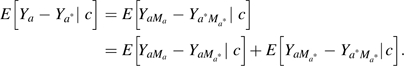
We extend the definitions of direct and indirect effects (1, 2) in causal inference from the risk difference to the odds ratio scale. On the risk difference scale, the total effect, conditional on C = c, comparing exposure level a with a^*, is defined by $E[Y_a-Y_{a^{*}}|c]$ and compares the average outcome in stratum C = c if A had been set to a with the average outcome in stratum C = c if A had been set to a^*. On the odds ratio (OR) scale, the total effect (TE), conditional on C = c, comparing exposure level a with a^*, is defined by

and compares the odds of outcome Y = 1 in stratum C = c if A had been a with the odds of outcome Y = 1 in stratum C = c if A had been a^*. In the context of the cardiovascular example, if we let a = 1 denote the estrogen therapy and a^* = 0 denote no therapy, then ${\text{OR}}_{1,0|c}^{\text{TE}}$ would be the odds ratio for cardiovascular disease comparing estrogen therapy with no therapy for individuals with covariate values c.

As with the total causal effect, we can also define direct and indirect effects on either the risk difference or the odds ratio scale. We will adopt the definitions and nomenclature of Pearl (2) for the risk difference scale and extend these concepts to the odds ratio scale. On the risk difference scale, the controlled direct effect, conditional on C = c, comparing exposure level a with a^* and fixing the mediator to level m, is defined by $E[Y_{am}-Y_{a^{*}m}|c]$ and captures the effect of exposure A on outcome Y, intervening to fix M to m. On the odds ratio scale, one could define the conditional controlled direct effect (CDE) as

If A is a binary, this is 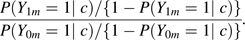. Note that these conditional controlled direct effects may vary with m when there is interaction between the effects of A and M on the odds ratio scale. In the cardiovascular example, ${\text{OR}}_{1,0|c}^{\text{CDE}}\left(m\right)$ would denote the odds ratio for cardiovascular disease comparing therapy and no therapy with serum lipid concentrations fixed at level m.

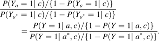
The so-called “natural direct effect” (2) or “pure direct effect” (1) differs from the controlled direct effect in that the intermediate M is set to the level $M_{a^{*}}$, the level it would have naturally been under some reference condition for the exposure, $A=a^{*}$; the natural direct effect, conditional on C = c, on the risk difference scale thus takes the form $E[Y_{a{M}_{a^{*}}}-Y_{a^{*}{M}_{a^{*}}}|c]$. The natural direct effect thus captures the effect of the exposure, estrogen therapy, on the outcome, cardiovascular disease, intervening to set the mediator, serum lipid concentration, to the level it would have been under the reference exposure level (e.g., no estrogen therapy). The conditional natural direct effect (NDE) odds ratio can be defined analogously and takes the form

On the odds ratio scale, the conditional natural direct effect can be interpreted as comparing the odds, conditional on C = c, of the outcome Y if exposure had been a, but if the mediator had been fixed to $M_{a^{*}}$ (i.e., to what it would have been if exposure had been a^*) to the odds, conditional on C = c, of the outcome Y if exposure had been a^* but if the mediator had been fixed at the same level $M_{a^{*}}$. This would capture the odds ratio for cardiovascular disease comparing therapy with no therapy intervening to set the serum lipid concentration to the level it would have been for each subject had they not had estrogen therapy.

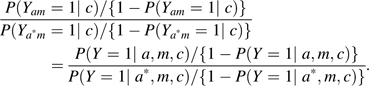
One can similarly define a natural indirect effect. On the risk difference scale, the conditional natural indirect effect can be defined as $E[Y_{a{M}_a}-Y_{a{M}_{a^{*}}}\left|c\right]$, which compares, conditional on C = c, the effect of the mediator at levels M_a and $M_{a^{*}}$ on the outcome when exposure A is set to a. The conditional natural indirect effect (NIE) can be defined analogously on the odds ratio scale as

On the odds ratio scale, the conditional natural indirect effect can be interpreted as comparing the odds, conditional on C = c, of the outcome Y if exposure had been a but if the mediator had been fixed to M_a (i.e., to what it would have been if exposure had been a) to the odds, conditional on C = c, of the outcome Y if exposure had been a but if the mediator had been fixed to $M_{a^{*}}$ (i.e., to what it would have been if exposure had been a^*). The natural indirect effect odds ratio thus captures the odds ratio for cardiovascular disease comparing serum lipid concentration under therapy and no therapy if the subject had in fact had estrogen therapy. As discussed elsewhere, controlled direct effects are often of greater interest in policy evaluation (2, 10), whereas natural direct and indirect effects are often of greater interest in evaluating the action of various mechanisms (10, 11). Note that throughout this paper we will consider all effects conditional on the covariates C, and we will thus use expressions such as “natural direct effect” and “conditional natural direct effect” interchangeably.

On the risk difference scale, natural direct and indirect effects have the property that the total effect $E[Y_a-Y_{a^{*}}|c]$ decomposes into a natural direct and indirect effect:

The decomposition holds even when there are nonlinearities and interactions. On the odds ratio scale, the natural direct and indirect effects also have a decomposition property. On the odds ratio scale, the odds ratio for the total effect decomposes into a product of odds ratios for the natural direct and indirect effect:

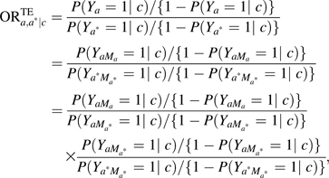where the first expression in the product is the natural indirect effect odds ratio, ${\text{OR}}_{a,a^{*}|c}^{\text{NIE}}\left(a\right)$, and the second expression is the natural direct effect odds ratio, ${\text{OR}}_{a,a^{*}|c}^{\text{NDE}}\left(a^{*}\right)$. On the log scale, this is . The ratio, 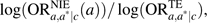, thus constitutes a measure of the proportion of the effect of the exposure mediated by the intermediate on the log odds scale. If the outcome is rare, one can use as a measure of the proportion mediated on the risk difference scale. We have given formulas for the “pure natural direct effect” and the “total natural indirect effect” (1); refer to the Web Appendix, which is posted on the Journal’s Web site (http://aje.oxfordjournals.org/) for further discussion of these measures and for analogous formulas for the “total natural direct effect” and the “pure natural indirect effect” (1).

Under certain assumptions that the set of covariates C contains all relevant confounding variables, the direct and indirect effects can be identified with observed data. We will follow the exposition of VanderWeele (12) and VanderWeele and Vansteelandt (9) on the identification assumptions proposed by Pearl (2). These identification assumptions were presented to identify direct and indirect effects on the risk difference scale but they apply also to the odds ratio scale.

To identify total effects, it is generally assumed that, conditional on some set of measured covariates C, the effect of exposure A on outcome Y is unconfounded; in counterfactual notation, this is $Y_a{\displaystyle \coprod }A|C$, where we use the independence symbol ∐ to denote that Y_a is independent of A conditional on C. In practice, to make this assumption more plausible, a researcher will attempt to collect data on a sufficiently rich set of covariates C to try to control for confounding of the exposure-outcome relation. If this assumption holds, then the odds ratio for the total causal effect, ${\text{OR}}_{a,a^{*}|c}^{\text{TE}}$, is identified and can be estimated from the data using

The left-hand side is the odds ratio for the total causal effect, ${\text{OR}}_{a,a^{*}|c}^{\text{TE}}$; the right-hand side is an expression that can be estimated from the data.

Controlled direct effects on the risk difference or risk ratio scale are identified if conditioning on the set of covariates C suffices to control for confounding of both the exposure-outcome and the mediator-outcome relations. In counterfactual notation, these 2 assumptions can, respectively, be written as that for all a and m,

(1)

(2)

Assumption 1 is similar to the assumption of no-unmeasured confounding assumption for total effects. Assumption 2 requires that, conditional on {A, C}, there is no unmeasured confounding for the mediator-outcome relation. If assumption 1 is satisfied but assumption 2 fails (i.e., if there is mediator-outcome confounding), then estimators for the direct and indirect effect will in general be biased (1, 2, 13, 14). Thus, in the cardiovascular example, if U denoted some aspect of diet that was associated with serum lipid levels and was also associated with cardiovascular disease, then it would be necessary to control for U in estimating the direct effect of estrogen therapy on cardiovascular disease controlling for serum lipid levels. If estrogen therapy were randomized, then its effect on serum lipid concentrations only or on cardiovascular disease only could be estimated without control for U but, when the direct effect of estrogen therapy on cardiovascular disease controlling for serum lipid concentrations is of interest, data on U would be needed.

Unfortunately, in many studies using mediation analysis, little attention is given to data collection for variables confounding the mediator-outcome relation. Effort is often made to collect data on some set of covariates C that suffice to control for confounding of the exposure-outcome relation so that assumption 1 is satisfied, but this will not ensure that assumption 2 is satisfied. As noted above, when there are mediator-outcome confounding variables that are unmeasured or for which control has not been made, estimates of direct and indirect effects will generally be biased. In epidemiologic research for which questions of mediation are of interest, greater effort should be made to collect data on potential mediator-outcome confounders. When these assumptions 1 and 2 do not hold, then sensitivity analysis for mediation for violations of the no-unmeasured confounding assumptions should be used (15, 16). If assumptions 1 and 2 hold, then the controlled direct effect on the risk difference scale and on the odds ratio scale is identified, and ${\text{OR}}_{a,a^{*}|c}^{\text{CDE}}\left(m\right)$ is then given by

For the identification of natural direct and indirect effects, additional assumptions are needed. Natural direct and indirect effects will be identified if, in addition to assumptions 1 and 2, the following 2 assumptions hold, that for all a, a^*, and m,

(3)

(4)

Assumption 3 can be interpreted as that, conditional on C, there is no unmeasured confounding for the exposure-mediator relation. Assumption 4 will hold if confounding for the mediator-outcome relation can be controlled for by some set of baseline covariates C, so that there is no effect of exposure A that confounds the mediator-outcome relation (i.e., no effect L of exposure A that itself affects both M and Y). Thus, assumption 4 would be violated in the case of Figure 2. In some settings, assumption 4 may be plausible if the mediator M occurs shortly after the exposure A (9). If, however, there is a variable L that is an effect of A and affects both M and Y, then assumption 4 is violated and natural direct and indirect effects will not in general be identified (17), irrespective of whether data are available on L. In such settings, it may still be possible to identify controlled direct effect odds ratios, but alternative statistical approaches such as marginal structural models (12, 18, 19) or structural nested models (20–24) will generally be needed. Note that none of assumptions 1–4 can be tested by using data; a researcher will have to rely on subject matter knowledge in evaluating them. In the next section, we will show how natural direct and indirect effects can be estimated in a relatively straightforward manner using regression.

Figure 2.

Example of mediation with exposure A, mediator M, outcome Y, covariates C, and a mediator-outcome confounder L that is itself affected by the exposure.

REGRESSION ANALYSIS FOR DIRECT AND INDIRECT EFFECT ODDS RATIOS

In this section, we describe a simple regression technique that can be used to estimate controlled direct effect and natural direct and indirect effect odds ratios when the assumptions above hold. The estimation technique for controlled direct effect odds ratios will require only assumptions 1 and 2 and will make use of a single logistic regression. The estimation technique for natural direct and indirect effect odds ratios will require assumptions 1–4 above and will combine the results of a linear and logistic regression to obtain the effects of interest; the estimation technique for natural direct and indirect effects will also require that the outcome Y is rare so that odds ratios approximate risk ratios, which allows one to obtain particularly simple formulae. We consider a setting in which the mediator M is continuous and the outcome Y is dichotomous. We have described a similar approach for continuous outcomes elsewhere (9). Derivations for the results below are given in the Web Appendix.

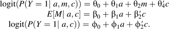
Consider the use of the following 2 models, a logistic regression for the outcome Y (with no A × M product term) and a linear regression for the mediator M:

(5)

and

(6)

where the error term for the linear regression for M is normally distributed with constant variance. If assumptions 1–4 hold and if regression models 5 and 6 are correctly specified, then the controlled and natural direct effect and natural indirect effect odds ratios are given by

where the approximation holds to the extent the rare outcome assumption holds. These expressions essentially use θ₁ for the direct effect and θ₂β₁ for the indirect effect, and these expressions are also often used in the social science literature for mediation analysis with a dichotomous outcome (25, 26). The use of models 5 and 6 along with the expressions above is often referred to as the “Baron-Kenny” approach to mediation (26). A related approach, common in both the epidemiologic literature and the social science literature, consists of regressing Y on A, M, C as in model 5 and then examining whether the coefficient for A is different from that obtained when Y is regressed on A and C alone, such as the folllowing:

The difference between coefficients for A, ϕ₁ − θ₁, is sometimes interpreted as an indirect effect. The traditional “proportion explained” methods (27–30) are closely related and use (ϕ₁ − θ₁)/ϕ₁ as the measure of interest, again effectively relying on the difference between the 2 coefficients. In the included Appendix, we in fact show that, under assumptions 1–4, correct specification of models 5 and 6, and a rare outcome, these 2 approaches to mediation analysis with a dichotomous outcome are essentially equivalent with ϕ₁ − θ₁ ≈ θ₂β₁. The results above provide a formal counterfactual interpretation of these various effect measures. An alternative measure of the “proportion explained” proposed by Wang et al. (31) is, under certain exchangeability assumptions, similar to a natural indirect effect (32).

However, a limitation of all of the standard approaches is that they presuppose that there is no statistical interaction on the odds ratio scale between A and M in the logistic model for Y. When such A × M interactions are present and are ignored, the logistic regression model 5 will not be correctly specified, and the difference ϕ₁ − θ₁ does not carry a straightforward interpretation as an indirect causal effect; the definition of an indirect effect essentially breaks down within the standard Baron-Kenny approach when such interactions are present (33). Hafeman (34) has also recently documented the biases that can arise with the traditional “proportion explained” methods when used in multiplicative models for a dichotomous outcome in which interaction terms are omitted. Here, we show how the regression approach can be extended to allow for interaction. Specifically, suppose that, instead of model 5, the following model, which includes an A × M product term, is used:

(7)

If assumptions 1–4 hold and if the regression models 6 and 7 are correctly specified and the outcome is rare, then the controlled direct effect and natural indirect effect odds ratios are given, respectively, by

(8)

(9)

The formula for the controlled direct effect odds ratio requires that assumptions 1 and 2 hold and that model 7 is correctly specified; no rare outcome assumption is required. The formula for the natural indirect effect odds ratio requires that assumptions 1–4 hold, that models 6 and 7 are correctly specified, and that the outcome Y is rare. An estimator can also be given for the natural direct effect odds ratio (refer to the Web Appendix material) but is more complicated because, when there is interaction between A and M in the logistic model for Y, the natural direct effect will be different for subjects with different covariate values C. Model 7 and expressions 8 and 9 essentially generalize the Baron-Kenny approach to allow for exposure-mediator interactions.

Ninety-five percent confidence intervals for the controlled direct effect odds ratio in expression 8 and the natural indirect effect odds ratio in expression 9 can be computed by using standard regression output and are given, respectively, by

and

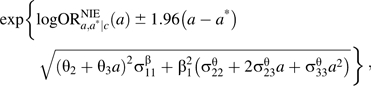where ${\text{σ}}_{ij}^{\text{β}}$ is the covariance between and in model 6, and ${\text{σ}}_{ij}^{\text{θ}}$ is the covariance between and in model 7; these covariances are given in the regression output of standard statistical software. Alternatively, standard errors for expressions 8 and 9 could be obtained by bootstrapping.

Expressions 8 and 9 generalize mediation analysis with a dichotomous outcome to settings in which there may be interactions on the odds ratio scale between the exposure and mediator of interest. The standard approach of omitting the θ₃am product term in assessing mediation is highly problematic when correct specification of a logistic regression model for Y requires the product term. When there is in fact such interaction between A and M, ignoring this (as is often done) can result in highly misleading inferences concerning mediation. If, for example, the direction of the association between A and Y differs for different levels of m and if the θ₃am term in model 7 is omitted, the resulting estimate of the exposure coefficient θ₁ may be close to 0 because of averaging. This might result in a researcher's concluding that the effect of A on Y is largely mediated by M, when in fact all that is the case is that there is an interaction between the effects of A and M on Y. At the very least, epidemiologists, before applying the standard approach, should test whether θ₃ = 0 in the regression model 7 and should consider whether the no-unmeasured-confounding assumptions described above are satisfied. If there is evidence that θ₃ ≠ 0, then this standard approach of merely including the mediator in a regression for the outcome Y to obtain direct and indirect effects should not be used. The approach described above, however, of using both models 6 and 7 could still be used when there is an interaction between A and M in model 7.

ODDS RATIOS FOR MEDIATION ANALYSIS IN CASE-CONTROL STUDIES

In this section, we describe how the above approach can be adapted when using case-control data. The case-control setting is of particular importance in mediation analysis with a dichotomous outcome because often, if the outcome is rare, it will be infeasible to conduct a cohort study with a sufficient number of individuals with the outcome. When data are used from a case-control study design, the estimators of (θ₁, θ₂, θ₃, θ₄) obtained from logistic regression 7 using case-control data will consistently estimate the same parameters of a logistic regression using cohort data. This well-known result is what justifies the use of logistic regression when analyzing odds ratios in case-control studies for total effects; when logistic regression is used, the case-control study design can effectively be ignored. Note that a logistic, not a log-linear model, is being used. In a case-control study, estimation of model 7 is thus straightforward. However, when fitting the linear regression model 6 for the mediator M using case-control data, the case-control study design cannot be ignored. It is nevertheless possible to adapt the approach to the estimation of direct and indirect effects described above in a relatively straightforward manner if the prevalence of the outcome Y is known. We will denote this prevalence by π. We assume it is known by design so that sampling variability for π is neglible. Also, let p denote the proportion of cases in the case-control study (i.e., the ratio of the number of cases in the study to the sum of the numbers of cases and controls in the study). If we fit a linear regression of M on A and C using the case-control data but weighting each case by π / p and each control by , then the coefficients obtained in this weighted regression will give consistent estimators of (β₀, β₁, β₂) obtained in a linear regression of M on A and C using data from a cohort study of the same population (35). Once (θ₁, θ₂, θ₃, θ₄) are obtained from the logistic regression and (β₀, β₁, β₂) are obtained from a weighted linear regression, the estimation of direct and indirect effects can then proceed using the formulas given in expressions 8 and 9 above.

ILLUSTRATION AND SIMULATIONS

As another example of mediation and to illustrate the approach we have described, we reanalyzed a previously reported study (36) with residence in a damp and moldy dwelling as the exposure, depression as the outcome, and perception of control over one's home as the mediator. A logistic regression model was fit for depression as a function of perception of control, dampness or mold exposure, and other individual and housing variables, as reported in Shenassa et al. (36), and a linear regression model was fit for perception of control as a function of the exposure and the same individual and housing variables, each time using generalized estimating equations to adjust for possible correlation between measurements from residents sharing the same dwelling. Allowing for the possibility of an interaction, the natural indirect effect of an increase in dampness or mold exposure from none to minimal, minimal to moderate, and moderate to extensive on the risk of depression corresponds to odds ratios of 1.03 (95% confidence interval (CI): 0.94, 1.14), 1.04 (95% CI: 0.95, 1.13), and 1.06 (95% CI: 0.93, 1.35). Standard analyses, ignoring such interactions, gave corresponding natural indirect effect odds ratios of 1.04 (95% CI: 0.99, 1.10), 1.04 (95% CI: 0.99, 1.09), and 1.04 (95% CI: 0.99, 1.19), respectively. Considering that no significant evidence of an interaction between dampness or mold exposure and perception of control was found (P = 0.91, 0.89, and 0.22 for minimal, moderate, and extensive dampness or mold exposure, respectively, relative to no exposure), the fact that these results are very similar is not surprising.

We also use data from this study as the basis for simulation experiments exploring bias and coverage probabilities when outcome prevalence is not rare or when exposure-mediator interactions are ignored. Table 1 shows (on the log odds scale) the bias, empirical standard error (ESE), average of the estimated standard errors (SSEs), and coverage of 95% confidence intervals for the natural indirect effects log odds ratios with a = 1 and a^* = 0, as based on 1,000 simulated data sets. Outcome and mediator data conditional on the observed exposure and covariates in the study by Shenassa et al. (36) were generated by using the data-generating models obtained in the previous analysis. In Table 1, the first 5 simulation experiments correspond to varying outcome prevalence. They demonstrate that the proposed estimates of the natural indirect effect odds ratio, while theoretically valid only at low outcome means, give good approximations even at larger prevalences for the data-generating mechanism underlying the data of Shenassa et al. The next 4 experiments evaluate the impact of exposure-mediator interactions. Here, the magnitude θ₃ = −0.22 was chosen to equal −2θ₂/3 and thus to generate a potentially substantial bias in the natural indirect effect odds ratio at a = 3, which was the largest observed exposure value. As theoretically expected, ignoring exposure-mediator interactions when they are present can generate a substantial bias in the indirect effect estimates. In the final 4 experiments β₁ and σ were increased 5 times (Ψ = 5 in Table 1) to give indirect effects of a larger magnitude; here, violations of the rare-outcome assumption do lead to bias.

Table 1.

Simulation Results for Natural Indirect Effects for Bias, Empirical and Estimated Standard Errors, and Coverage Probabilities of 95% Confidence Intervals, With Varying Outcome Prevalence and Exposure-Mediator Interactions

E(Y)	θ3	Ψ	Without Interaction				With Interaction
			Bias	ESE	SSE	Cov	Bias	ESE	SSE	Cov
0.01	0.0035	1	0.0011	0.014	0.015	95.6	0.00027	0.015	0.015	95.0
0.25			0.00024	0.0046	0.0048	94.0	0.00039	0.0047	0.0048	94.3
0.5			−0.00021	0.0043	0.0043	94.7	0.00046	0.0044	0.0044	94.8
0.75			−0.00057	0.0045	0.0047	92.5	0.00039	0.0047	0.0049	94.4
0.089			0.0055	0.0059	0.0059	95.3	0.00018	0.0059	0.0059	94.7
	−0.22		0.0032	0.0058	0.0058	93.6	0.000036	0.0058	0.0058	96.4
	0.22		0.0045	0.0069	0.0069	93.7	0.00047	0.0066	0.0067	95.7
	−0.44		0.013	0.0061	0.0062	42.7	−0.00010	0.0069	0.0069	95.0
	0.44		0.0095	0.0088	0.0088	84.2	0.0010	0.0080	0.0083	95.1
0.01	0.0035	5	0.014	0.028	0.024	93.8	0.0059	0.028	0.024	95.9
0.25			0.013	0.019	0.016	87.7	0.015	0.019	0.016	85.6
0.5			0.019	0.017	0.016	79.1	0.023	0.018	0.016	72.9
0.75			0.021	0.017	0.015	73.7	0.026	0.018	0.017	64.5

Abbreviations: Cov, coverage probability; ESE, empirical standard error; E(Y), outcome prevalence; SSE, estimated standard error; θ₃, exposure-mediator interaction; Ψ, variance factor.

Table 2 shows related results for the natural direct effects log odds ratios. Results are similar as for natural indirect effects: Coverage is poor when an exposure-mediator interaction is present and ignored but reasonable when the approach with the interaction is used. With natural direct effects, in the final 4 experiments, we see that the bias of the proposed estimator due to failure of the rare-outcome assumption can be more sizeable than that of the standard approach in settings in which the exposure-mediator interaction is in fact negligible.

Table 2.

Simulation Results for Natural Direct Effects for Bias, Empirical and Estimated Standard Errors, and Coverage Probabilities of 95% Confidence Intervals, With Varying Outcome Prevalence and Exposure-Mediator Interactions

E(Y)	θ3	Ψ	Without Interaction				With Interaction
			Bias	ESE	SSE	Cov	Bias	ESE	SSE	Cov
0.01	0.0035	1	0.020	0.15	0.13	94.7	−0.0053	0.16	0.15	95.1
0.25			0.016	0.033	0.032	93.9	0.00029	0.036	0.036	96.6
0.5			0.015	0.033	0.030	92.1	0.0030	0.035	0.032	94.2
0.75			0.020	0.035	0.040	90.2	0.010	0.041	0.037	93.7
0.089			−0.0026	0.053	0.047	95.0	−0.019	0.057	0.052	93.3
	−0.22		−0.071	0.043	0.060	78.6	−0.0085	0.049	0.065	95.9
	0.22		0.078	0.042	0.059	53.8	0.0051	0.050	0.066	93.9
	−0.44		−0.11	0.042	0.074	72.1	−0.0060	0.050	0.081	95.0
	0.44		0.039	0.078	0.039	7.8	0.014	0.095	0.054	94.1
0.01	0.0035	5	0.039	0.18	0.14	94.6	0.0048	0.18	0.14	96.4
0.25			−0.0093	0.040	0.035	93.8	0.072	0.055	0.044	64.7
0.5			−0.0052	0.035	0.032	94.7	0.13	0.062	0.049	23.2
0.75			−0.00094	0.039	0.038	95.3	0.18	0.087	0.068	21.9

Abbreviations: Cov, coverage probability; ESE, empirical standard error; E(Y), outcome prevalence; SSE, estimated standard error; θ₃, exposure-mediator interaction; Ψ, variance factor.

Results from simulations of case-control data with prevalence-weighted regressions for the mediator followed a similar pattern as for the estimator of the natural indirect effect: bias if one ignores a substantial exposure-mediator interaction when present and bias when the rare-outcome assumption is violated.

DISCUSSION

The 2 most common pitfalls with mediation analysis in the epidemiologic literature are 1) ignoring possible mediator-outcome confounding and 2) ignoring possible interactions between the effects of exposure and mediator on the outcome. Either pitfall can lead to severely biased estimates and incorrect conclusions concerning mediation. With regard to pitfall 1, we would recommend that, when questions of mediation are of interest, greater attention be paid to the collection of data on variables that may confound the mediator-outcome relation and that sensitivity analysis be used when it is not possible to make control for such confounders (15, 16). As noted above, the no-unmeasured-confounding assumptions used for the identification of direct and indirect effects cannot be verified with data, so researchers need to carefully evaluate these using subject matter knowledge and sensitivity analysis techniques. With regard to pitfall 2, we would recommend that, before proceeding with what has become a routine approach of simply including an intermediate variable in a regression to assess mediation, investigators first examine whether there is interaction between the effects of the exposure and the mediator on the outcome. If there is interaction, then the routine approach of omitting the product term from the regression model should be avoided; instead, the product term can be included and, provided that the outcome is rare, the approach we have described in this paper can be used.

Several further comments merit attention. First, we have seen that, although mediation analysis is more difficult when there is interaction between the exposure and the mediator (1, 33, 37), this interaction can in fact be accommodated. Our simple formulae did, however, assume no interaction between the confounders and the treatment or mediator; other estimation techniques (16) could be used if there are confounder-exposure interactions; other identification approaches are also possible when such interactions are present in their effects on the mediator (21, 38). Second, the methods described above require a rare outcome; this was necessary in the derivations and also circumvents collapsibility issues with odds ratios (39); some existing work considers or could be adapted for non-rare outcomes (16, 40); future work will consider settings in which the outcome is not rare and compare power, bias, and efficiency properties of the estimators. Third, we have considered the setting of a dichotomous outcome and a continuous mediator. When the mediator M is dichotomous, rather than continuous, a somewhat similar approach to the one described here could potentially be used, but the analytic formulas for mediated effects no longer take quite as simple a form. Fourth, in genetic epidemiology, the extent to which genetic variants affect an outcome (e.g., lung cancer) through intermediate phenotypes (e.g., nicotine addiction) has recently been a topic of interest (41–43); the approach we have described here for case-control studies can be applied to address such questions in genetics research.

Glossary

Abbreviations

CDE

controlled direct effect

CI

confidence interval

ESE

empirical standard error

NDE

natural direct effect

NIE

natural indirect effect

OR

odds ratio

SSE

estimated standard error

TE

total effect

APPENDIX

Comparison With Dichotomous Outcome Mediation Analysis in the Social Science Literature

As noted in the text, the approach often used in the social sciences (25) involves using regressions such as models 5 and 6, along with a regression of Y on just A (and C):

Potential confounding variables are often ignored in many of the analyses in the social sciences in which the exposure is randomized (even though the mediator is not randomized), and thus the set C is sometimes assumed to be empty. With these regression models, there are then 2 approaches to estimation typically used for the mediated effect (i.e., indirect effect). The first uses β₁θ₂ as a measure of the mediated effect, and the second uses ϕ₁ − θ₁ as a measure of the mediated effect. The 2 measures will often not coincide. In the text, we showed that, under the assumptions of 1) a rare outcome, 2) normally distributed error in regression 6, 3) identification conditions 1–4 holding, and 4) no interaction between a and m in the regression model 5, the quantity β₁θ₂ is approximately equal to the log of the natural indirect effect odds ratio, 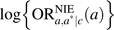. In fact, if the outcome is rare and the error term for regression model 6 is normally distributed (with constant variance σ²), then it will be the case that β₁θ₂ ≈ ϕ₁−θ₁ since, under the rare-outcome assumption, we must have ${\text{ϕ}}_{\text{0}}+{\text{ϕ}}_{\text{1}}a+{\mathrm{\varphi }}_{\text{2}}\prime c=\text{logit}\left(P\right(Y=1|a,c))\approx \log \{P(Y=1|a,c\left)\right\}$, and thus we have that

Because this holds for all a, we must have that ϕ₁ ≈ (θ₁ + θ₂β₁) and thus ϕ₁ − θ₁ ≈ θ₂β₁.

If, however, the outcome is not rare or if the error term in regression model 6 is heteroscedastic or not normally distributed, then the 2 quantities β₁θ₂ and ϕ₁ −θ₁ need not be approximately equal. Furthermore, in that case, neither β₁θ₂ nor ϕ₁ −θ₁ may warrant an interpretation as an indirect effect. Moreover, if the set C does not satisfy the no-unmeasured-confounding assumptions described in the text, then β₁θ₂ and ϕ₁ −θ₁ may both be biased for the true log natural indirect effect odds ratio even if the outcome is rare and the error term in model 6 is normally distributed with constant variance. Finally, this standard approach in the social science literature applies only if there are no interactions between A and M in regression model 5; the approach described in the text, however, can still be employed when such interactions are present.

References

- 1.Robins JM, Greenland S. Identifiability and exchangeability for direct and indirect effects. Epidemiology. 1992;3(2):143–155. doi: 10.1097/00001648-199203000-00013. [DOI] [PubMed] [Google Scholar]
- 2.Pearl J. Proceedings of the Seventeenth Conference on Uncertainty and Artificial Intelligence. San Francisco, CA: Morgan Kaufmann; 2001. Direct and indirect effects; pp. 411–420. [Google Scholar]
- 3.Mendelsohn ME, Karas RH. The protective effects of estrogen on the cardiovascular system. N Engl J Med. 1999;340(23):1801–1811. doi: 10.1056/NEJM199906103402306. [DOI] [PubMed] [Google Scholar]
- 4.Bush TL, Barrett-Connor E, Cowan LD, et al. Cardiovascular mortality and noncontraceptive use of estrogen in women: results from the Lipid Research Clinics Program Follow-up Study. Circulation. 1987;75(6):1102–1109. doi: 10.1161/01.cir.75.6.1102. [DOI] [PubMed] [Google Scholar]
- 5.Rubin DB. Formal modes of statistical inference for causal effects. J Statist Plan Inf. 1990;25(3):279–292. [Google Scholar]
- 6.Hernán MA. A definition of causal effect for epidemiological research. J Epidemiol Community Health. 2004;58(4):265–271. doi: 10.1136/jech.2002.006361. [DOI] [PMC free article] [PubMed] [Google Scholar]
- 7.Pearl J. Causality: Models, Reasoning, and Inference. 2nd ed. Cambridge, United Kingdom: Cambridge University Press; 2009. [Google Scholar]
- 8.VanderWeele TJ. Concerning the consistency assumption in causal inference. Epidemiology. 2009;20(6):880–883. doi: 10.1097/EDE.0b013e3181bd5638. [DOI] [PubMed] [Google Scholar]
- 9.VanderWeele TJ, Vansteelandt S. Conceptual issues concerning mediation, interventions and composition. Stat Interface. 2009;2(4):457–468. [Google Scholar]
- 10.Robins JM. Semantics of causal DAG models and the identification of direct and indirect effects. In: Green P, Hjort NL, Richardson S, editors. Highly Structured Stochastic Systems. New York, NY: Oxford University Press; 2003. pp. 70–81. [Google Scholar]
- 11.Joffe M, Small D, Hsu CY. Defining and estimating intervention effects for groups that will develop an auxiliary outcome. Stat Sci. 2007;22(1):74–97. [Google Scholar]
- 12.VanderWeele TJ. Marginal structural models for the estimation of direct and indirect effects. Epidemiology. 2009;20(1):18–26. doi: 10.1097/EDE.0b013e31818f69ce. [DOI] [PubMed] [Google Scholar]
- 13.Judd CM, Kenny DA. Process analysis: estimating mediation in treatment evaluations. Eval Rev. 1981;5(5):602–619. [Google Scholar]
- 14.Cole SR, Hernán MA. Fallibility in estimating direct effects. Int J Epidemiol. 2002;31(1):163–165. doi: 10.1093/ije/31.1.163. [DOI] [PubMed] [Google Scholar]
- 15.VanderWeele TJ. Bias formulas for sensitivity analysis for direct and indirect effects. Epidemiology. 2010;21(4):540–551. doi: 10.1097/EDE.0b013e3181df191c. [DOI] [PMC free article] [PubMed] [Google Scholar]
- 16.Imai K, Keele L, Tingley D. Pyschol Methods. A general approach to causal mediation analysis. In press. [DOI] [PubMed] [Google Scholar]
- 17.Avin C, Shpitser I, Pearl J. Proceedings of the International Joint Conferences on Artificial Intelligence. San Francisco, CA: Morgan Kaufman; 2005. Identifiability of path-specific effects; pp. 357–363. [Google Scholar]
- 18.Robins JM, Hernán MA, Brumback B. Marginal structural models and causal inference in epidemiology. Epidemiology. 2000;11(5):550–560. doi: 10.1097/00001648-200009000-00011. [DOI] [PubMed] [Google Scholar]
- 19.van der Laan MJ, Petersen ML. Direct effect models. International Journal of Biostatistics. Vol. 4(issue 1) doi: 10.2202/1557-4679.1064. article 23. Berkeley, CA: Berkeley Electronic Press; 2008. [DOI] [PubMed] [Google Scholar]
- 20.Robins JM. Testing and estimation of direct effects by reparameterizing directed acyclic graphs with structural nested models. In: Glymour C, Cooper GF, editors. Computation, Causation, and Discovery. Menlo Park, CA: AAAI Press/Cambridge, MA: The MIT Press; 1999. pp. 349–405. [Google Scholar]
- 21.Ten Have TR, Joffe MM, Lynch KG, et al. Causal mediation analyses with rank preserving models. Biometrics. 2007;63(3):926–934. doi: 10.1111/j.1541-0420.2007.00766.x. [DOI] [PubMed] [Google Scholar]
- 22.Goetgeluk S, Vansteelandt S, Goetghebeur E. Estimation of controlled direct effects. J R Stat Soc B. 2008;70(5):1049–1066. [Google Scholar]
- 23.Joffe MM, Greene T. Related causal frameworks for surrogate outcomes. Biometrics. 2009;65(2):530–538. doi: 10.1111/j.1541-0420.2008.01106.x. [DOI] [PubMed] [Google Scholar]
- 24.Vansteelandt S. Estimating direct effects in cohort and case-control studies. Epidemiology. 2009;20(6):851–860. doi: 10.1097/EDE.0b013e3181b6f4c9. [DOI] [PubMed] [Google Scholar]
- 25.MacKinnon DP. An Introduction to Statistical Mediation Analysis. New York, NY: Lawrence Erlbaum Associates; 2008. [Google Scholar]
- 26.Baron RM, Kenny DA. The moderator-mediator variable distinction in social psychological research: conceptual, strategic, and statistical considerations. J Pers Soc Psychol. 1986;51(6):1173–1182. doi: 10.1037//0022-3514.51.6.1173. [DOI] [PubMed] [Google Scholar]
- 27.Freedman LS, Graubard BI, Schatzkin A. Statistical validation of intermediate endpoints for chronic diseases. Stat Med. 1992;11(2):167–178. doi: 10.1002/sim.4780110204. [DOI] [PubMed] [Google Scholar]
- 28.Lin DY, Fleming TR, De Gruttola V. Estimating the proportion of treatment effect explained by a surrogate marker. Stat Med. 1997;16(13):1515–1527. doi: 10.1002/(sici)1097-0258(19970715)16:13<1515::aid-sim572>3.0.co;2-1. [DOI] [PubMed] [Google Scholar]
- 29.Li Z, Meredith MP, Hoseyni MS. A method to assess the proportion of treatment effect explained by a surrogate endpoint. Stat Med. 2001;20(21):3175–3188. doi: 10.1002/sim.984. [DOI] [PubMed] [Google Scholar]
- 30.Chen C, Wang H, Snapinn SM. Proportion of treatment effect (PTE) explained by a surrogate marker. Stat Med. 2003;22(22):3449–3459. doi: 10.1002/sim.1575. [DOI] [PubMed] [Google Scholar]
- 31.Wang Y, Taylor JM. A measure of the proportion of treatment effect explained by a surrogate marker. Biometrics. 2002;58(4):803–812. doi: 10.1111/j.0006-341x.2002.00803.x. [DOI] [PubMed] [Google Scholar]
- 32.Taylor JM, Wang Y, Thiébaut R. Counterfactual links to the proportion of treatment effect explained by a surrogate marker. Biometrics. 2005;61(4):1102–1111. doi: 10.1111/j.1541-0420.2005.00380.x. [DOI] [PubMed] [Google Scholar]
- 33.Kaufman JS, MacLehose RF, Kaufman S. A further critique of the analytic strategy of adjusting for covariates to identify biologic mediation [electronic article] Epidemiol Perspect Innov. 2004;1(1):4. doi: 10.1186/1742-5573-1-4. [DOI] [PMC free article] [PubMed] [Google Scholar]
- 34.Hafeman DM. “Proportion explained”: a causal interpretation for standard measures of indirect effect? Am J Epidemiol. 2009;170(11):1443–1448. doi: 10.1093/aje/kwp283. [DOI] [PubMed] [Google Scholar]
- 35.van der Laan MJ. Estimation based on case-control designs with known prevalence probability. International Journal of Biostatistics. Vol. 4(issue 1) doi: 10.2202/1557-4679.1114. article 17. Berkeley, CA: Berkeley Electronic Press; 2008. [DOI] [PubMed] [Google Scholar]
- 36.Shenassa ED, Daskalakis C, Liebhaber A, et al. Dampness and mold in the home and depression: an examination of mold-related illness and perceived control of one's home as possible depression pathways. Am J Public Health. 2007;97(10):1893–1899. doi: 10.2105/AJPH.2006.093773. [DOI] [PMC free article] [PubMed] [Google Scholar]
- 37.VanderWeele TJ. Mediation and mechanism. Eur J Epidemiol. 2009;24(5):217–224. doi: 10.1007/s10654-009-9331-1. [DOI] [PubMed] [Google Scholar]
- 38.Dunn G, Bentall R. Modelling treatment-effect heterogeneity in randomized controlled trials of complex interventions (psychological treatments) Stat Med. 2007;26(26):4719–4745. doi: 10.1002/sim.2891. [DOI] [PubMed] [Google Scholar]
- 39.Greenland S, Robins JM, Pearl J. Confounding and collapsibility in causal inference. Stat Sci. 1999;14(1):29–46. [Google Scholar]
- 40.Huang B, Sivaganesan S, Succop P, et al. Statistical assessment of mediational effects for logistic mediational models. Stat Med. 2004;23(17):2713–2728. doi: 10.1002/sim.1847. [DOI] [PubMed] [Google Scholar]
- 41.Wacholder S, Chatterjee N, Caporaso N. Intermediacy and gene-environment interaction: the example of CHRNA5-A3 region, smoking, nicotine dependence, and lung cancer. J Natl Cancer Inst. 2008;100(21):1488–1491. doi: 10.1093/jnci/djn380. [DOI] [PMC free article] [PubMed] [Google Scholar]
- 42.Chanock SJ, Hunter DJ. Genomics: when the smoke clears…. Nature. 2008;452(7187):537–538. doi: 10.1038/452537a. [DOI] [PubMed] [Google Scholar]
- 43.Vansteelandt S, Goetgeluk S, Lutz S, et al. On the adjustment for covariates in genetic association analysis: a novel, simple principle to infer direct causal effects. Genet Epidemiol. 2009;33(5):394–405. doi: 10.1002/gepi.20393. [DOI] [PMC free article] [PubMed] [Google Scholar]