Non-crossing large-margin probability estimation and its application to robust SVM via preconditioning

Abstract

Many large-margin classifiers such as the Support Vector Machine (SVM) sidestep estimating conditional class probabilities and target the discovery of classification boundaries directly. However, estimation of conditional class probabilities can be useful in many applications. Wang, Shen, and Liu (2008) bridged the gap by providing an interval estimator of the conditional class probability via bracketing. The interval estimator was achieved by applying different weights to positive and negative classes and training the corresponding weighted large-margin classifiers. They propose to estimate the weighted large-margin classifiers individually. However, empirically the individually estimated classification boundaries may suffer from crossing each other even though, theoretically, they should not.

In this work, we propose a technique to ensure non-crossing of the estimated classification boundaries. Furthermore, we take advantage of the estimated conditional class probabilities to precondition our training data. The standard SVM is then applied to the preconditioned training data to achieve robustness. Simulations and real data are used to illustrate their finite sample performance.

1 Introduction

Binary classification or discrimination handles data with a binary response, where we are interested in studying the relationship between a p-vector predictor x and a binary response y ∈ {−1, +1}. In particular we seek a classification rule to predict the binary response for an arbitrary input predictor. A well-known traditional likelihood-based statistical approach is the logistic regression, which tries to estimate the conditional probability p(x) = P(Y = 1∣X = x) and make prediction ŷ = 1 if p̂(x) > 1/2 and −1 otherwise for any x. See McCullagh and Nelder (1989) for a detailed introduction to logistic regression.

Recently many margin-based classifiers have been proposed in the literature. Examples include the support vector machine (SVM) (Vapnik, 1998; Cortes and Vapnik, 1995), Boosting (Freund and Schapire, 1997; Friedman, Hastie, and Tibshirani, 2000), ψ-learning (Shen, Tseng, Zhang, and Wong, 2003), etc. By sidestepping the conditional class probability estimation and targeting directly at classification, many margin-based classification methods may yield good classification performance. However, one main drawback of some margin-based classifiers such as the SVM is that they are not able to provide an estimator of the conditional class probability directly. As argued by Wang, Shen, and Liu (2008), the conditional class probability itself is of significant scientific interest in that it provides us the confidence level of our class prediction.

To provide class probability estimation for large-margin classifiers, Wang et al. (2008) proposed an interval estimation method to estimate the conditional class probability. By noting that {x : f̂(x) = 0} estimates the Bayes boundary {x : p(x) – 1/2 = 0} for a margin-based classifier sign(f̂(x)), they propose to run different weighted margin-based classification individually to estimate Bayes boundaries {x : p(x) – p = 0} for a prespecified grid of p. Each weighted classifier can estimate whether p(x) > p or not without estimating p(x) itself. In this way, an interval estimator is obtained by bracketing the conditional class probability p(x). Their approach is nonparametric in the sense that it does not make any parametric assumption on p(x).

Theoretically Bayes boundaries {x : p(x) – p = 0} for different p should not cross each other. To bracket the conditional class probability, we estimate them using the classification boundaries of the weighted margin-based classifiers based on a finite training data set. Thus the individually estimated boundaries may unavoidably cross each other, especially when the training sample size is small. This crossing phenomenon was also pointed out by Wang et al. (2008). Their probability bracketing method cannot avoid crossing. In this work, we address this crossing issue and provide a technique to enforce non-crossing of the estimated classification boundaries. With this technique, we can ensure non-crossing of the estimated boundaries, at least over the convex hull of the training data points, where the training data convex hull represents the smallest convex hull in the input space which contains all the training data points.

As mentioned earlier, the estimated conditional class probability can provide us with some confidence of our prediction for any x. Our method yields an estimate of p(x_i) for each training dataset point (x_i, y_i). For a clean training data with a low noise level, we generally expect a training observation with class probability estimate bigger (smaller) than 0.5 to have class label y_i = +1 (y_i = −1, respectively), especially so for those with probabilities close to 1 or 0. A training point with large (small) probability estimate and class label y_i = −1 (y_i = +1, respectively) is typically an outlier. It is known that such outliers may pull the classification boundaries towards themselves and as a result can reduce the classification performance (Wu and Liu, 2007). In order to improve classification performance in such cases, we propose to precondition the training data set based on the estimated conditional class probabilities; i.e., we change the class labels of potential outliers to the corresponding correct class labels. After preconditioning the training set, any standard margin-based classifier may be applied to obtain a robust classification rule.

In the literature there are some other robust margin-based classifiers such as ψ-learning (Shen et al., 2003 and Liu and Shen, 2006) and the robust truncated-hinge-loss SVM (RSVM) (Wu and Liu, 2007). These robust methods typically involve non-convex optimization, which is more expensive to solve than convex minimization. Our pre-conditioning method serves as another technique to achieve robustness. Compared to ψ-learning and the RSVM, our preconditioned SVM can avoid non-convex optimization.

The rest of the article is organized as follows. Some background on the SVM and weighted SVM is given in Section 2. Section 3 presents our technique which provides non-crossing probability estimation. In Section 4, we propose to robustify margin-based classifiers via preconditioning. Simulation and real data analysis are reported in Sections 5 and 6.

2 Standard and weighted SVMs

For binary classification, a training data set {(x_i, y_i) : i = 1, 2, ⋯ , n} is typically given where n is the sample size, x_i ∈ R^p is the p-dimensional input vector, and y_i ∈ {−1, +1} is a binary response. The goal is to construct a function f(·) whose sign will be used as the classification rule, namely ŷ = sign(f(x)) for any new input x.

The SVM was first invented from the idea of searching for the optimal separating hyperplane using an elegant margin interpretation (Vapnik, 1998; Cristianini and Shawe-Taylor, 2000). The idea can be traced back to the method of portraits (Vapnik and Lerner, 1963). It is now known that the SVM is equivalent to solving the following optimization

$$\underset{f(·)}{\min }\left\{\sum _{i=0}^{n}H(y_{i}f({\mathit{x}}_i))+\lambda J(f)\right\},$$ (1)

where H(η) = max(0, 1 – η) is the hinge loss function and J(f) is the roughness penalty of f(·) (Wahba, 1998). Here y_if(x_i) is the functional margin. A positive functional margin value indicates correct classification and the corresponding 0 – 1 loss can be expressed as I(y_if(x_i)) > 0. Besides the SVM, many other classifiers can be fit into the regularization framework. In fact the hinge loss can be replaced by a general large-margin loss V (u) satisfying the condition that V (u) is non-increasing in u, thereby penalizing small margin values more than large margin values. Some common loss functions include the exponential loss V (u) = exp(−u) (Friedman et al., 2000), the logistic loss V (u) = log(1 + exp(−u)) (Lin et al., 2000; Zhu and Hastie, 2005), the ψ-loss V (u) = 1 – sign(u) if u ≥ 1 or u < 0, 2(1 – u) otherwise (Shen et al., 2003), etc. Figure 1 displays some common large margin loss functions.

Figure 1.

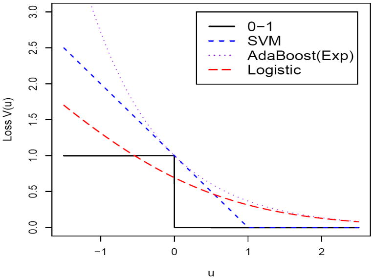
Plot of several common binary large margin loss functions.

Lin (2002) showed that the theoretical minimizer of the hinge loss is sign(p(x) – 0.5). Consequently, the SVM only targets at the Bayes classification boundary asymptotically. As a result, the SVM boundary {x : f̂(x) = 0} estimates the Bayes boundary {x : p(x) = 0.5}, where f̂(·) is the solution to (1). Lin et al. (2002) proposed a weighted hinge loss by giving different weights for the positive and negative classes and solves a weighted version of (1), namely,

$$\min \left\{(1-\pi )\sum _{i:y_i=1}H(f({\mathit{x}}_i))+\pi \sum _{i:y_i=-1}H(-f({\mathit{x}}_i))+\lambda J(f)\right\}$$ (2)

for some π ∈ [0, 1]. It reduces to (1) when π = 1/2. The weighted SVM (2) was originally proposed to handle the problem of unequal representation of categories in the training sample or unequal costs for positive and negative misclassifications with π and 1 – π being the known costs for negative and positive classes, respectively. Interestingly, it turns out that the classification boundary of the optimizer f̂(·) of (2) estimates the Bayes boundary {x : p(x) = π}.

Motivated by the properties of a weighted loss function, Wang et al. (2008) proposed to solve (2) for many different π’s and, consequently, to estimate the conditional probability p(x) via bracketing the probability. For simplicity, they proposed to solve (2) individually over a grid 0 = π₁ < π₂ < ⋯ π_K = 1. The corresponding algorithm for estimating the conditional class probability can be summarized as follows.

Wang et al.’s Algorithm (2008):

1. Initialize π_k = (k – 1)/(K – 1) for k = 1, 2, … , K.

2. Train a weighted large-margin classifier for π_k by solving (2) and denote the solution as f̂_πk(x) for k = 1, 2, … , K.

3. For each x, compute $k^{\ast }=k^{\ast }(\mathit{x})\triangleq \max \{k:{\widehat{f}}_{{\pi }_k}(\mathit{x})\ge 0\}$ and $k_{\ast }=k_{\ast }(\mathit{x})\triangleq \min \{k:{\widehat{f}}_{{\pi }_k}(\mathit{x})\le 0\}$. The estimated conditional class probability is given by $\widehat{p}(\mathit{x})=\frac{1}{2}({\pi }_{k^{\ast }}+{\pi }_{k_{\ast }})$.

When the estimated classification boundaries {x : f̂_πk(x) = 0} do not cross each other, k^*(x) and k_*(x) should satisfy |k^*(x) – k_*(x)| ≤ 1 for any x. Unfortunately individually optimized boundaries for different π_k’s may cross each other, especially for small training samples. As a result, one may have contradictory probability estimation using multiple individually optimized classification functions. To solve the crossing problem, we propose a technique to enforce non-crossing constraints in this paper. Furthermore, we propose to robustify the SVM via preconditioning by taking advantage of the estimated probabilities.

3 Non-crossing class probability estimation

As discussed in Section 2, the weighted SVM with π and 1 – π being weights for negative and positive classes targets at the Bayes boundary {x : p(x) = π}. Note that {x : p(x) ≥ π_j} ⊂ {x : p(x) ≥ π_l} for ∀π_j > π_l. As a result, classification boundaries with different π’s should not cross each other theoretically. However, the estimated classification boundaries may cross each other if each weighted SVM is calculated separately.

In this section, we present a new technique to ensure that the estimated classification boundaries do not cross each other. We illustrate the non-crossing technique first in the linear case in Section 3.1. Its extension to the nonlinear case via the kernel trick is then discussed in Section 3.2. As mentioned in Section 2, we aim to solve (2) for many different π_k’s (0 = π₁ < π₂ < ⋯ < π_K = 1) to obtain an estimator for the conditional class probability. Denote by k₀ the index such that π_k0 is the closest to 1/2 among all different π_k’s, namely, $\left|{\pi }_{k_0}-1/2\right|=\underset{1\le k\le K}{\min }\left|{\pi }_k-1/2\right|$.

3.1 Linear boundaries

By making the linearity assumption on the classification boundaries, we assume that f_k(x) = x^Tw_k + b_k corresponds to π_k for k = 1, 2, ⋯ , K. For the linear function f_k(x), we choose its roughness penalty to be the 2-norm penalty, namely $J(f_k)={\mathit{w}}_k^T{\mathit{w}}_k$.

Our non-crossing algorithm begins with estimating the classification boundary corresponding to π_k0 by solving the following optimization problem

$$\min \left\{(1-{\pi }_{k_0})\sum _{i:y_i=1}{[1-({\mathit{x}}_i^T\mathit{w}+b)]}_{+}+{\pi }_{k_0}\sum _{i:y_i=-1}{[1+({\mathit{x}}_i^T\mathit{w}+b)]}_{+}+\lambda \sum _{j=1}^p{w}_j^2\right\},$$ (3)

where the regularization parameter can be tuned either using a separate independent tuning data set or cross-validation. Denote the corresponding estimator by ŵ_k0 and b̂_k0.

For any k > k₀, we require that the classification boundary corresponding to π_k does not cross that of π_k–1 within the convex hull of the data points. In particular, the convex hull H_convex(x₁, x₂, ⋯ , x_n) represents the smallest convex set in the input data space which contains all the training points x₁, x₂, ⋯ , x_n. Since the region of the training data is a set where the testing data points are likely to fall in, our technique aims to avoid crossing of different boundaries in H_convex(x₁, x₂, ⋯ , x_n). To achieve this goal, we solve the following constrained optimization problem

$$\min \left\{(1-{\pi }_k){\sum }_{i:y_i=1}{[1-{\mathit{x}}_i^T\mathit{w}+b)]}_{+}+{\pi }_k{\sum }_{i:y_i=-1}{[1+({\mathit{x}}_i^T\mathit{w}+b)]}_{+}+\lambda {\sum }_{j=1}^p{w}_j^2\right\},\mathrm{s.t.}{\mathit{x}}^T\mathit{w}+b\le 0\mathrm{for\; any}\mathit{x}\in \{\mathit{x}:{\mathit{x}}^T{\widehat{\mathit{w}}}_{k-1}+{\widehat{b}}_{k-1}=0\}\cap H_{\mathit{convex}}({\mathit{x}}_1,{\mathit{x}}_2,\cdots ,{\mathit{x}}_n),$$ (4)

where ŵ_k–1 and b̂_k–1 represent the solution corresponding to π_k–1.

A a remark, we note that a direct way for calculation of the constraint set in (4) is to find the set of intersections of all pairwise line segments between two training data points with the surface. However, the computation can be greatly reduced by the fact that the restriction is satisfied as long as x^Tw + b ≤ 0 holds for any x in the intersecion between the surface x ∈ {x : x^Tŵ_k–1 + b̂ = 0} and the edges of the convex hull H_convex(x₁, x₂, ⋯ , x_n). Furthermore, only a small subset of all pairwise line segments are edges of the convex hull. Thus, we need to find all edges of H_convex(x₁, x₂, ⋯ , x_n) and enumerate the intersection between these edges and the surface x ∈ {x : x^T ŵ_k–1+b̂ = 0}.

Notice that any edge of H_convex(x₁, x₂, ⋯ , x_n) can be represented as a segment between two training data points. If p < n, we can first derive all facets of the convex hull and each edge should fall in one or more of the facets. A facet of the convex hull with p vertice lies in a hyperplane, such that all training data points fall either on the hyperplane or on the same side of that hyperplane. If p ≥ n, all data points are vertices and any pairwise line segment between two training points is an edge of H_convex(x₁, x₂, ⋯ , x_n).

Once the points in the intersection in (4) are enumerated, the constrained weighted SVM given in (4) can be implemented using quadratic programming (QP).

Similarly we can estimate the classification boundary corresponding to π_k for k < k₀ by solving

$$\min \left\{(1-{\pi }_k){\sum }_{i:y_i=1}{[1-{\mathit{x}}_i^T\mathit{w}+b)]}_{+}+{\pi }_k{\sum }_{i:y_i=-1}{[1+({\mathit{x}}_i^T\mathit{w}+b)]}_{+}+\lambda {\sum }_{j=1}^p{w}_j^2\right\},\mathrm{s.t.}{\mathit{x}}^T\mathit{w}+b\ge 0\mathrm{for\; any}\mathit{x}\in \{\mathit{x}:{\mathit{x}}^T{\widehat{\mathit{w}}}_{k+1}+{\widehat{b}}_{k+1}=0\}\cap H_{\mathit{convex}}({\mathit{x}}_1,{\mathit{x}}_2,\cdots ,{\mathit{x}}_n).$$ (5)

Note that we begin with the center π_k0 and move to the two ends sequentially to estimate the classification boundaries. By using constraints (4) and (5), it is guaranteed that our estimated classification boundaries do not cross each other within the convex hull of our data. Then Step 3 of Wang et al. (2008)’s algorithm can be applied to estimate the conditional class probability. The main difference of our new algorithm is to enforce non-crossing constraints on the corresponding classification boundaries.

3.2 Nonlinear boundaries

Nonlinear classification can be achieved by using the kernel trick. Denote by K(·, ·) a reproducing kernel function. Then by the Representer Theorem, the classification function can be expressed as $f(\mathit{x})={\sum }_{i=1}^n{\theta }_{i}K({\mathit{x}}_i,\mathit{x})+\beta$. In this case the roughness penalty is given by $J(f)={\sum }_{i=1}^n{\sum }_{i^{\prime }=1}n{\theta }_i{\theta }_{i^{\prime }}K({\mathit{x}}_i,{\mathit{x}}_{i^{\prime }})$ (Wahba, 1998). Letting F denote the reproducing kernel Hilbert space (RKHS), the weighted SVM (2) becomes

$$\underset{f\in F}{\min }\left\{(1-\pi )\sum _{i:y_i=1}H(f({\mathit{x}}_i))+\pi \sum _{i:y_i=-1}H(-f({\mathit{x}}_i))+\lambda J(f)\right\}.$$ (6)

Once we plug the expressions of f(x) and J(f) into (6), the optimization reduces to a QP problem with respect to θ = (θ₁, θ₂, ⋯ , θ_n)^T and β. To further simplify the problem, let x̃_i = (K(x_i, x₁), K(x_i, x₂), ⋯ , K(x_i, x_n))^T. Then $f({\mathit{x}}_i)={\stackrel{\sim }{\mathit{x}}}_i^T\mathit{\theta }+\beta$. Therefore the non-crossing technique for the linear case can be applied to the kernel case as well.

Denote by K a n × n matrix with (i, j)-element being K(x_i, x_j). We solve

$${\min }_{\mathit{\theta },\beta }\left\{(1-{\pi }_{k_0}){\sum }_{i:y_i=1}{[1-({\stackrel{\sim }{\mathit{x}}}_i^T\mathit{\theta }+\beta )]}_{+}+{\pi }_{k_0}{\sum }_{i:y_i=-1}{[1+({\stackrel{\sim }{\mathit{x}}}_i^T\mathit{\theta }+\beta )]}_{+}+\lambda {\mathit{\theta }}^T\mathit{K}\mathit{\theta }\right\}$$

and denote the corresponding solutions as θ̂_k0 and β̂_k0. Then, for k > k₀, we sequentially solve

$${\min }_{\mathit{\theta },\beta }\left\{(1-{\pi }_k){\sum }_{i:y_i=1}{[1-({\stackrel{\sim }{\mathit{x}}}_i^T\mathit{\theta }+\beta )]}_{+}+{\pi }_k{\sum }_{i:y_i=-1}{[1+({\stackrel{\sim }{\mathit{x}}}_i^T\mathit{\theta }+\beta )]}_{+}+\lambda {\sum }_{j=1}^p{w}_j^2\right\},\mathrm{s.t.}{\stackrel{\sim }{\mathit{x}}}^T\mathit{\theta }+\beta \le 0\mathrm{for\; any}\stackrel{\sim }{\mathit{x}}\in \{\stackrel{\sim }{\mathit{x}}:{\stackrel{\sim }{\mathit{x}}}^T{\widehat{\mathit{\theta }}}_{k-1}+{\widehat{\beta }}_{k-1}=0\}\cap H_{\mathit{conver}}({\stackrel{\sim }{\mathit{x}}}_1,{\stackrel{\sim }{\mathit{x}}}_2,\cdots ,{\stackrel{\sim }{\mathit{x}}}_n)$$ (7)

and denote the corresponding solutions as θ̂_k and β̂_k; for k < k₀, we sequentially solve

$${\min }_{\mathit{\theta },\beta }\left\{(1-{\pi }_k){\sum }_{i:y_i=1}{[1-({\stackrel{\sim }{\mathit{x}}}_i^T\mathit{\theta }+\beta )]}_{+}+{\pi }_k{\sum }_{i:y_i=-1}{[1+({\stackrel{\sim }{\mathit{x}}}_i^T\mathit{\theta }+\beta )]}_{+}+\lambda {\sum }_{j=1}^p{w}_j^2\right\},\mathrm{s.t.}{\stackrel{\sim }{\mathit{x}}}^T\mathit{\theta }+\beta \ge 0\mathrm{for\; any}\stackrel{\sim }{\mathit{x}}\in \{\stackrel{\sim }{\mathit{x}}:{\stackrel{\sim }{\mathit{x}}}^T{\widehat{\mathit{\theta }}}_{k+1}+{\widehat{\beta }}_{k+1}=0\}\cap H_{\mathit{conver}}({\stackrel{\sim }{\mathit{x}}}_1,{\stackrel{\sim }{\mathit{x}}}_2,\cdots ,{\stackrel{\sim }{\mathit{x}}}_n)$$ (8)

Note that calculation of the set {x̂ : x̂^Tθ̂_k+1+β̂_k+1 = 0}⋂H_convex(x̂₁, x̂₂, ⋯ , x̂_n) is similar to that of the linear case. The difference here is that we consider the n-dimensional kernel space instead of the p-dimensional linear space.

The estimated classification boundary for π_k is given by $\{\mathit{x}:{\sum }_{i=1}^n{\widehat{\theta }}_{\mathit{ki}}K({\mathit{x}}_i,\mathit{x})+{\widehat{\beta }}_k=0\}$, where θ_ki is the ith element of θ_k. The constraints (7) and (8) guarantee the desired non-crossing. Once the classification boundaries with different weights are obtained, Step 3 of Wang et al.’s algorithms can be applied to estimate the conditional class probability as in the linear case.

4 Robust learning via preconditioning

In Section 3, we present a technique to estimate classification functions with different weights and without crossing to estimate class probabilities. In this section, we propose to make use of the estimated class probabilities to precondition the training data. This preconditioning operation may help to remove potential outliers and consequently yield more robust classifiers.

In the literature, there is some existing work suggesting that the SVM may not be robust to outliers or mislabeled data points (Shen et al. 2003). One main reason is that the hinge loss used in the SVM is unbounded. Consequently, potential outliers or mislabeled data points may pull the classification boundary towards themselves and thus reduce the classification performance.

For a training data set with a low noise level, we expect that most data points fall in their corresponding class sets. A training point is likely to be an outlier if it is far from its own class. Specifically, for a non-outlier data point x_i with y_i = 1 (y_i = −1), its estimated conditional class probability p̂(x_i) should be likely to be larger (smaller, respectively) than 0.5. This gives us a potential method to identify outliers. If there are some data points x_i with y_i = 1 and p̂(x_i) close to zero or some data points x_i with y_i = −1 and p̂(x_i) close to one, then these points (x_i, y_i)’s are likely to be outliers. The outliers can be mislabeled data due to error or a result of sampling biases.

Once we have identified outliers, we can correct them by flipping their binary response from y_i to −y_i and train the standard SVM with the modified training data set. In this way, we are able to remove the effect of these outliers from deteriorating the performance of the SVM. We call this technique preconditioning. In the literature, preconditioning has been applied in the regression problems. In particular, Paul, Bair, Hastie and Tibshirani (2008) proposed to first estimate the regression function to yield a preconditioned response variable. Then they apply standard variable selection techniques to the preconditioned response variable. They argued that the preconditioning step helps to get better variable selection performance. Our preconditioning method is similar to that of Paul et al. (2008) in the sense that we generate a more “clean” binary response variable first and then apply the standard large-margin classifiers to achieve robustness.

We now give more details of our technique of preconditioning. We first choose a prespecified preconditioning level π̃, which can be any number between 0 and 0.5. For our training data {(x_i, y_i), i = 1, 2, ⋯ , n}, we estimate the conditional class probability p̂(x_i) for each data point using our non-crossing technique. For any x_i, we precondition the binary response by defining

$${\stackrel{\sim }{y}}_i=\{\begin{array}{ll}-1& \mathrm{if}\widehat{p}({\mathit{x}}_i)\in [0,\stackrel{\sim }{\pi })\\ y_i& \mathrm{if}\widehat{p}({\mathit{x}}_i)\in [\stackrel{\sim }{\pi },1-\stackrel{\sim }{\pi }]\\ 1& \mathrm{if}\widehat{p}({\mathit{x}}_i)\in (1-\stackrel{\sim }{\pi },1].\end{array}$$

Here π̃ ∈ [0, 0.5) controls the level of preconditioning. A large π̃ indicates an aggressive preconditioning while a small π̃ means that preconditioning is used conservatively. When π̃ = 0, no preconditioning is applied and our preconditioned SVM reduces to the standard SVM.

Once preconditioning has been applied, we train the standard SVM (1) over the preconditioned training data set {(x_i, ỹ_i), i = 1, 2, ⋯ , n} to get our final classification rule. Letting f̃_π̃(·) be the solution of (1) using the preconditioned data with the optimal tuning parameter λ, then our final classification rule is sign(f̃_π̃(x)).

Compared to other robust large-margin classifiers such as ψ-learning (Shen et al, 2003) and the RSVM (Wu and Liu, 2007), our preconditioning method is another technique to robustify the SVM without nonconvex optimization. In Section 5, we perform a simulation study to compare the performance of our preconditioned SVM with that of the RSVM.

5 Simulation

In this section we use several simulated examples to illustrate the performance of our proposed methods. Examples 1, 2, 3 and 4 are linear while examples 5 and 6 are nonlinear. For the linear case, we use the 2-norm penalty. Example 1 compares the estimated conditional class probability using Wang et al. (2008) with that of our proposed non-crossing version. Examples 2-6 are used to show improvement of the preconditioned SVM over the standard SVM. In all simulated examples, we use an independent tuning set {(x_i,tune, y_i,tune), i = 1, 2, ⋯ , n_tune} to select the regularization parameter λ in (2) by minimizing

$$(1-{\pi }_k)\sum _{i:y_{i,\mathit{tune}}=1}H({\widehat{f}}_{\lambda }({\mathit{x}}_{i,\mathit{tune}}))+{\pi }_k\sum _{i:y_{i,\mathit{tune}}=-1}H(-{\widehat{f}}_{\lambda }({\mathit{x}}_{i,\mathit{tune}}))$$

over a grid of λ, where f̂_λ (·) denotes the solution of the weighted SVM with the tuning parameter λ.

5.1 Linear learning

Example 1 (Class probability estimation comparison)

In this example, the two dimensional predictor x = (x₁, x₂)^T is uniformly distributed over the square {(x₁, x₂)^T : |x₁| + |x₂| ≤ 2}. Conditional on X = x, Y takes +1 with probability p(x) = exp(4(x₁ + x₂))/(1+exp(4(x₁+x₂))) and −1 with probability 1–exp(4(x₁+x₂))/(1+exp(4(x₁+x₂))), namely, (X, Y) comes from a logistic regression model. We set the sample size n = 100, and π_k = 0:01(k – 1) for k = 1, 2, ⋯ , 101. Independent tuning and test data sets are generated to tune the regularization parameter λ and evaluate performance, respectively. Both Wang et al.’s method and our non-crossing version for conditional class probability estimation are applied. As the true conditional class probability is known in this simulation, we report the empirical generalized Kullback-Leibler (eGLK) loss over both the training and test data sets. The eGLK loss of a probability estimator p̂(x) for a set {(x_i, y_i), i = 1, 2, ⋯ , n} with true conditional class probability p(x), is defined as

$$\mathrm{eGLK}(p,\widehat{p})=\frac{1}{n}\sum _{i=1}^n\left(p({\mathit{x}}_i)\log \frac{p(\mathit{x})}{\widehat{p}(\mathit{x})}+(1-p({\mathit{x}}_i))\log \frac{1-p(\mathit{x})}{1-\widehat{p}(\mathit{x})}\right).$$

Average eGLK of the training set and test set over 100 repetitions are reported in Table 1 with standard errors in parentheses. We can see slight improvement of our non-crossing version, however the improvement is not statistically significant. Nevertheless, the noncrossing version leads to better statistical interpretation.

Table 1.

Simulation results for Example 1

	Non-crossing		Wang et al.
	training	test	training	test
GKL	2.0639 (.0896)	2.1501 (.0924)	2.0907 (.0894)	2.1591 (.0908)

For a typical sample, we compare Wang et al.’s method with our new non-crossing version by plotting the estimated classification boundaries for different π_k’s in Figure 2. The left panel corresponds to Wang et al.’s method while the right panel is for our new non-crossing version. It is clear from the plot that the estimated classification boundaries do cross each other for some π_k’s if they are estimated individually. However, by enforcing the non-crossing constraints, our new version leads to non-crossing classification boundaries which give better interpretation. This figure demonstrates the usefulness of the non-crossing constraints.

Figure 2.

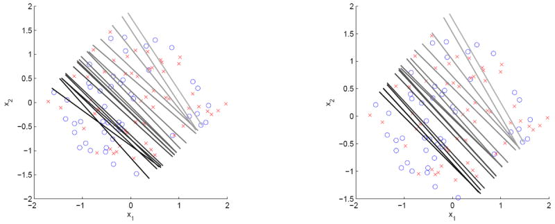
Estimated classification boundaries for different π_k in a typical sample of Example 1 with π = 0.05, 0.06, 0.07, 0.08, 0.09, 0.10, 0.20, 0.30, 0.40, 0.50, 0.60, 0.70, 0.80, 0.90, 0.96, 0.97, 0.98, 0.99: Wang et al.’s method is in the left panel and our new non-crossing version is in the right panel.

Example 2

In this example, the data {(x_i, y_i), i = 1, 2, ⋯ , n} are generated as i.i.d. copies of (X, Y) with X being uniformly distributed over the square {(x₁, x₂) : |x₁| + |x₂| ≤ 2} and Y = sign(x₁ + x₂) with probability 0:9 and Y = −sign(x₁ + x₂) with probability 0.1. We set the sample size n = 100. An independent tuning set of size n is used to select the tuning parameter. In this probability estimation step, we set π_k = 0:05(k – 1) for k = 1, 2, ⋯ , 21. Over 100 repetitions, average testing errors over an independent test set of size 100_n and corresponding standard errors are reported in Table 2 for the standard SVM, our preconditioned SVMs with different preconditioning levels π̃, and the RSVM. Using the standard SVM as the baseline, the difference, ratio and relative improvement are reported as well. For example, when π̃ = 0.1, the difference and ratio improvements are given by 0.1289 – 0.1294 = −0.0005, 0.1289/0.1294 = 0.9961 and (0.1294 – 0.1289)/(0.1294 – 0.1000) = 0.0172 (up to rounding error), respectively. From Table 2, we can see that our preconditioned SVM improves over the standard SVM at all different levels of preconditioning and the improvement is maximized at π̃ = 0.3. The RSVM leads to a slightly larger improvement using nonconvex optimization.

Table 2.

Simulation results of Example 2

	SVM	π̃							RSVM
		0.10	0.15	0.20	0.25	0.30	0.35	0.40
test error	.1294	.1289	.1286	.1244	.1228	.1222	.1224	.1243	.1215
SE	.0020	.0020	.0018	.0017	.0013	.0011	.0011	.0012	.0013
difference	.0000	-.0005	-.0008	-.0050	-.0066	-.0072	-.0070	-.0051	-.0079
ratio	1.0000	.9961	.9938	.9615	.9490	.9440	.9457	.9602	.9386
improvement	.0000	.0172	.0273	.1693	.2242	.2462	.2389	.1749	.2701

Example 3 (moderate dimension: d = 8)

In this example, we increase the dimensionality of the feature space to 8. The eight-dimensional predictor x = (x₁, x₂, ⋯ , x₈)^T is generated from the uniform distribution over $\{\mathit{x}:{\sum }_{j=1}^8|x_j|\le 8\}$. Conditional on X = x, $Y=\mathrm{sign}({\sum }_{j=1}^8{x}_j)$ with probability 0.9 and $Y=-\mathrm{sign}({\sum }_{j=1}^8{x}_j)$ with probability 0.1. The sample size is chosen to be n = 200. Simulation results based on 100 replications are reported in Table 3. The message is the similar to the previous example. In particular, our preconditioned SVM does better than the standard SVM but worse than the RSVM.

Table 3.

Simulation results of Example 3

	SVM	π̃							RSVM
		0.10	0.15	0.20	0.25	0.30	0.35	0.40
test error	.1496	.1497	.1466	.1404	.1370	.1370	.1378	.1417	.1284
SE	.0016	.0016	.0016	.0015	.0014	.0013	.0013	.0014	.0014
difference	.0000	.0000	-.0031	-.0092	-.0126	-.0126	-.0118	-.0079	-.0212
ratio	1.0000	1.0003	.9796	.9387	.9155	.9156	.9208	.9473	.8585
improvement	.0000	-.0009	.0615	.1848	.2549	.2545	.2387	.1590	.4268

Example 4 (high dimension: d = 50)

In this example, we increase the dimensionality of the feature space to 50. Predictors are independent of each other and are marginally distributed as the standard normal distribution. Conditional on X = x, $Y=\mathrm{sign}({\sum }_{j=1}^{50}{x}_j)$ with probability 0.9 and $Y=-\mathrm{sign}({\sum }_{j=1}^{50}{x}_j)$ with probability 0.1. The sample size is chosen to be n = 200. Simulation results are reported in Table 4. The message is very similar to the previous examples. However, the advantages of the robust methods are much smaller than before, possibly due to the difficulty of high dimension.

Table 4.

Simulation results of Example 4

	SVM	π̃							RSVM
		0.10	0.15	0.20	0.25	0.30	0.35	0.40
test error	.2433	.2433	.2433	.2430	.2412	.2395	.2407	.2444	.2382
SE	.0021	.0021	.0021	.0021	.0021	.0021	.0023	.0023	.0022
difference	.0000	.0000	-.0000	-.0003	-.0021	-.0038	-.0026	.0010	-.0051
ratio	1.0000	1.0000	1.0000	.9986	.9915	.9844	.9894	1.0043	.9789
improvement	.0000	.0000	.0001	.0023	.0145	.0265	.0179	-.0073	.0359

5.2 Kernel learning

Example 5

In this example we consider a nonlinear Bayes boundary. The two dimensional predictor x = (x₁, x₂)^T is uniformly distributed over the square {(x₁, x₂)^T : max(|x₁|, |x₂|) ≤ 2}. Conditional on X = x, the binary response Y takes sign $\mathrm{sign}(x_1^2+x_2^2-8/\pi )$ with probability 0:9 and $-\mathrm{sign}(x_1^2+x_2^2-8/\pi )$ with probability 0.1. Sample size n is set to be 100. We implement the nonlinear SVM using the kernel trick with the Gaussian kernel $K(\mathit{x},{\mathit{x}}^{\prime })=\exp (-{\parallel \mathit{x}-{\mathit{x}}^{\prime }\parallel }_2^2)$, where ${\parallel \mathit{x}\parallel }_2=\sqrt{x_1^2+x_2^2}$. Results over 100 repetitions are reported in Table 5. Interestingly, the RSVM performs slightly worse than the SVM for this example, while our preconditioned SVM improves over the standard SVM.

Table 5.

Simulation results of Example 5

	SVM	π̃							RSVM
		0.10	0.15	0.20	0.25	0.30	0.35	0.40
test error	.1652	.1650	.1628	.1612	.1593	.1576	.1565	.1577	.1766
SE	.0020	.0020	.0020	.0020	.0018	.0019	.0019	.0019	.0022
difference	.0000	-.0002	-.0024	-.0041	-.0059	-.0076	-.0088	-.0076	.0114
ratio	1.0000	.9985	.9852	.9754	.9640	.9541	.9470	.9542	1.0691
improvement	.0000	.0038	.0375	.0623	.0911	.1162	.1342	.1160	-.1751

Example 6

In this example, two-dimensional predictors are generated uniformly from the unit disc $\{(x_1,x_2):x_1^2+x_2^2<1\}$. Conditional on X = x, Y = sign(x₁) with probability 0.9 and Y = −sign(x₁) with probability 0.1. The sample size is chosen to be n = 100. A similar example was previously used by Shen et al. (2003).

Simulation results are reported in Table 6. In this example, both the RSVM and our preconditioned SVM give improvement over the standard SVM. Compared to the RSVM, our preconditioned SVM delivers more accurate classification accuracy.

Table 6.

Simulation results of Example 6

	SVM	π̃							RSVM
		0.10	0.15	0.20	0.25	0.30	0.35	0.40
test error	.1302	.1295	.1287	.1267	.1263	.1256	.1267	.1283	.1289
SE	.0013	.0013	.0013	.0014	.0015	.0013	.0013	.0013	.0014
difference	.0000	-.0007	-.0015	-.0035	-.0039	-.0046	-.0035	-.0019	-.0013
ratio	1.0000	.9947	.9886	.9733	.9702	.9648	.9731	.9854	.9903
improvement	.0000	.0231	.0491	.1152	.1287	.1517	.1161	.0630	.0418

It is worthwhile to point out that although both the RSVM and preconditioned SVM can yield more robust classifiers, it is interesting to see from our simulated examples that they perform differently for linear versus nonlinear examples. In particular, the RSVM generally works slightly better than the preconditioned SVM in linear examples, and the preconditioned SVM works better than the RSVM in kernel examples. Further investigation is needed to examine whether this pattern holds in general.

As a remark, we note that the value of π̃ greatly affects of the performance of our preconditioned SVM. The larger π̃ is, the more change we perform on the training data. In practice, one may use a data adaptive procedure to select π̃ to optimize the performance for the preconditioned SVM. For example, one may treat π̃ as a tuning parameter and select the value which gives the most accurate classification performance.

6 Liver disorder data

In this section we apply our preconditioned SVM to the dataset Liver-disorder. This dataset is available at the UCI Machine Learning Repository. More information can be found at the UCI webpage http://archive.ics.uci.edu/ml/index.html. It has a total of 345 observations with six predictor variables and a binary response.

To analyze the data, we first standardize each predictor variable to have mean zero and standard deviation one. Then we randomly split the dataset into training, tuning, and testing sets, each of size 115. As in Wu and Liu (2007), in order to study robustness of our preconditioned SVM for both the training and tuning sets, we contaminate the binary output by randomly choosing a fixed percent of their observations and changing the class output to the other class. Contamination with different percentages, perc = 0%, 5%, and 10%, are considered and applied to both the training and tuning sets, but not to the testing set.

To examine the performance of our proposed method, we apply both the standard linear SVM and our preconditioned linear SVM with different preconditioning levels π̃’s. Average testing errors over 10 random splitting are reported in Table 7 for different methods with corresponding standard errors in parentheses. For each different perc, the entry with boldface corresponds to the best performance and each entry with an underline indicates that it improves over the standard SVM. Table 7 shows that a relatively high level of preconditioning improves over the standard SVM either for the case without contamination (perc = 0%) or with contamination (perc = 5% or 10%). This clearly demonstrates that our preconditioned SVM is more robust than the standard SVM.

Table 7.

Numerical results of the Liver Disease data

perc	SVM	π̃
		0.10	0.15	0.20	0.25	0.30	0.35	0.40
0%	.3226 (.0112)	.3226 (.0112)	.3226 (.0112)	.3226 (.0112)	.3226 (.0112)	.3200 (.0107)	.3217 (.0110)	.3183 (.0127)
5%	.3670 (.0112)	.3670 (.0112)	.3670 (.0112)	.3670 (.0112)	.3670 (.0112)	.3678 (.0107)	.3487 (.0110)	.3452 (.0127)
10%	.3661 (.0214)	.3661 (.0214)	.3661 (.0214)	.3661 (.0214)	.3661 (.0214)	.3574 (.0187)	.3513 (.0170)	.3487 (.0149)

7 Discussion

The SVM only estimates the classification boundary without producing the class probability estimation. To get class probability estimation for the SVM, Wang et al. (2008) makes use of multiple weighted SVM boundaries to yield nonparametric class probability estimation. However, since each weighted SVM is calculated separately, different weighted classification boundaries may cross each other.

In this work, we first propose a technique to estimate different classification boundaries without crossing using weighted SVMs with constraints. Once the estimated conditional class probabilities are obtained, we make use of that to precondition our training data set. The operation of preconditioning may help to remove potential outliers. To get robust classifiers, we propose to apply the standard SVM on the preconditioned training data set. Our simulated and real examples clearly demonstrate that our preconditioned SVM improves over the standard SVM.

To estimate multiple classification boundaries, we only make use of the 2-norm penalty. However, when the dimensionality is large with many noise variables in the predictor, it is necessary to consider other penalties that are able to achieve variable selection, such as the LASSO penalty (Tibshirani, 1996; Zhu et al, 2004) and SCAD penalty (Fan and Li, 2001). It will be interesting to consider simultaneous classification and variable selection for the SVM as in Zhang, Liu, Wu, and Zhu (2008).

References

- Cortes C, Vapnik V. Support-vector networks. Machine Learning. 1995;20:273–279. [Google Scholar]
- Cristianini N, Shawe-Taylor J. An Introduction to Support Vector Machines and other Kernel-Based Learning Methods. Cambridge University Press; 2000. [Google Scholar]
- Fan J, Li R. Variable selection via nonconcave penalized likelihood and it oracle properties. Journal of American Statistical Association. 2001;96:1348–1360. [Google Scholar]
- Freund Y, Schapire R. A decision theoretic generalization of on-line learning and an application to boosting. Journal of Computer and System Sciences. 1997;55:119–139. [Google Scholar]
- Friedman JH, Hastie T, Tibshirani R. Additive logistic regression: a statistical view of boosting. Annals of Statistics. 2000;28:337–407. [Google Scholar]
- Lin X, Wahba G, Xiang D, Gao F, Klein R, Klein B. Smoothing Spline ANOVA Models for Large Data Sets With Bernoulli Observations and the Randomized GACV. The Annals of Statistics. 2000;28:1570–1600. [Google Scholar]
- Lin Y. Support vector machines and the Bayes rule in classification. Data Mining Know Disc. 2002;6:259–275. [Google Scholar]
- Lin Y, Lee Y, Wahba G. Support Vector Machines for classification in nonstandard situations. Machine Learning. 2002;46:191–202. [Google Scholar]
- Liu Y, Shen X. Multicategory ψ-learning. Journal of the American Statistical Association. 2006;101:500–509. [Google Scholar]
- McCullagh P, Nelder JA. Generalized linear models. 2. Chapman & Hall; London: 1989. [Google Scholar]
- Paul D, Bair E, Hastie T, Tibshirani R. Pre-conditioning for feature selection and regression in high-dimensional problems. Annals of Statistics. 2008;36(4):1595–1618. [Google Scholar]
- Shen X, Tseng GC, Zhang X, Wong WH. On ψ-learning. J Amer Statist Assoc. 2003;98:724–734. [Google Scholar]
- Tibshirani R. Regression shrinkage and selection via the lasso. Journal of the Royal Statistical Society, Series B. 1996;58:267–288. [Google Scholar]
- Vapnik V. Statistical learning theory. Wiley; 1998. [DOI] [PubMed] [Google Scholar]
- Vapnik V, Lerner A. Pattern recognition using generalized portrait method. Automation and Remote Control. 1963:24. [Google Scholar]
- Wahba G. Support vector machines, reproducing kernel Hilbert spaces, and randomized GACV. In: Scholkopf B, Burges CJC, Smola AJ, editors. Advances in Kernel Methods: Support Vector Learning. MIT Press; 1998. pp. 125–143. [Google Scholar]
- Wang J, Shen X, Liu Y. Probability estimation for large margin classifiers. Biometrika. 2008;95:149–167. [Google Scholar]
- Wu Y, Liu Y. Robust truncated-hinge-loss support vector machines. Journal of the American Statistical Association. 2007;102:974–983. [Google Scholar]
- Zhang HH, Liu Y, Wu Y, Zhu J. Variable selection for the multicategory SVM via sup-norm regularization. Electronic Journal of Statistics. 2008;2:149–167. [Google Scholar]
- Zhu J, Hastie T. Kernel Logistic Regression and the Import Vector Machine. Journal of Computational and Graphical Statistics. 2005;14:185–205. [Google Scholar]
- Zhu J, Rosset S, Hastie T, Tibshirani R. 1-norm support vector machines. Neural Information Processing Systems. 2004:16. [Google Scholar]