Improved Hidden Markov Models for Molecular Motors, Part 2: Extensions and Application to Experimental Data

Abstract

Unbiased interpretation of noisy single molecular motor recordings remains a challenging task. To address this issue, we have developed robust algorithms based on hidden Markov models (HMMs) of motor proteins. The basic algorithm, called variable-stepsize HMM (VS-HMM), was introduced in the previous article. It improves on currently available Markov-model based techniques by allowing for arbitrary distributions of step sizes, and shows excellent convergence properties for the characterization of staircase motor timecourses in the presence of large measurement noise. In this article, we extend the VS-HMM framework for better performance with experimental data. The extended algorithm, variable-stepsize integrating-detector HMM (VSI-HMM) better models the data-acquisition process, and accounts for random baseline drifts. Further, as an extension, maximum a posteriori estimation is provided. When used as a blind step detector, the VSI-HMM outperforms conventional step detectors. The fidelity of the VSI-HMM is tested with simulations and is applied to in vitro myosin V data where a small 10 nm population of steps is identified. It is also applied to an in vivo recording of melanosome motion, where strong evidence is found for repeated, bidirectional steps smaller than 8 nm in size, implying that multiple motors simultaneously carry the cargo.

Introduction

Tracking experiments on single molecular motors produce staircase data that contain a wealth of information such as the protein's step size, translocation speed and direction, rate of ATP turnover, and transitions between conformational states. However, much of this information can be difficult to extract owing to the poor signal/noise ratio (S/N) in these nanometer-scale measurements. Several approaches have been proposed in the past to interpret noisy motor protein recordings. These approaches range from conventional step detection using statistical tests (1) to a more sophisticated hidden Markov model-based algorithm (2). Here we extend the variable-stepsize hidden Markov model (VS-HMM) approach described in our previous article (3) to better account for the features of experimental data.

In experiments tracking molecular motors, each protein is labeled with a tag, such as a fluorescent molecule or a latex bead, whose position is monitored with a charge-coupled device (CCD) camera or a photodetector. If measurements are of sufficient time resolution then, the recording resembles a staircase composed of long dwell periods when the motor is bound to its substrate interrupted by instantaneous jumps when, for example, the protein hydrolyses ATP and undergoes conformational change. Because binding and hydrolysis events are stochastic events, the jumps in the protein's position occur at random times. The position reported by an electronic detector is updated at regular intervals (frames) and typically represents the average position of the tag during the frame interval.

We first wished to provide a better formal description of the measurement errors in such integrating detectors; the result is an extension to our previous algorithm, to yield what is now called the variable-stepsize, integrating-detector HMM (VSI-HMM). The incorporation of baseline drifts into the model is another extension which is described here. Finally, for determining dwell times in the presence of very high noise levels, the incorporation of prior knowledge, in the form of a prior probability function, is desirable. We have incorporated this, to yield a maximum a posteriori (MAP) estimation framework.

In this article, we describe these extensions to the hidden Markov model algorithms and compare the performance of the VSI-HMM with conventional step detection methods. Finally, the method is applied to experimental data where VS-HMM analysis uncovers small step sizes in myosin V in vitro motility and provides evidence for tug-of-war when multiple kinesins and dyneins operate simultaneously in vivo.

Theory

Review of the VS-HMM model

We first give a brief review of the notation of the VS-HMM model. The position of the molecular motor is sampled at discrete times t =1, 2,…T , where each unit of time represents a frame of the electronic camera. The measured position values are y_t, and the collection of all of the measurements is called Y. The true position is x_t ∈ {1, 2, … M}, which is mapped into the periodic variable u_t ∈ {1, 2, … m} to simplify the computations. The molecular state at time t is s_t ∈ {1, 2, … n} and the combination (s_t,u_t) of the molecular state and the position is called the composite state of the system.

In the Markov model, the probability of the transition from the composite state (i,u) at time t to the composite state (j, u+w) at t + 1 is given by c_ij(w). Thus, c_ij(0) is the probability of making the molecular transition from i to j with no change in position. Similarly, it is formally possible to have a position change of size w with no change of molecular state; this probability would be given by c_ii(w). In special cases, we therefore can construct models with only one molecular state by assigning nonzero values to c_ii(w). Such models carry out steps in position with Poisson-distributed dwell times. In all cases, c must satisfy the stochastic condition

$$\sum _{j=1}^n\sum _{w=-m/2}^{m/2-1}{c}_{ij}\left(w\right)=1.$$

The parameters of the hidden Markov model are the noise standard deviation σ₀, the initial probability π_iu (which is the probability of being in state i and position u at t = 1), and the transition probabilities c_ij(w). An additional parameter, which will be discussed below, is the vector of baseline vertices κ_r. All of the parameters are varied to maximize the likelihood L or, alternatively, the posterior probability.

Markov model extensions

The integrating-detector HMM

In the previous article (3), we modeled the measurement error by adding a Gaussian random variable g_t to the instantaneous motor position u_t, that is

$$y_t=u_t+g_t.$$

This would be correct if the continuous motion of the motor were sampled at discrete times. However, when a frame-transfer CCD camera is used for distance measurements, the single-molecule fluorescence measured at time t has been integrated for essentially the entire time interval from t–1 to t. A realistic model should take into account the integration time of the position measurement. To a very good approximation, the estimated position of the fluorophore will equal its average position over the (t−1, t] interval. Let η be the measurement duty cycle—the fraction of the time interval during which the optical signal is integrated. Then, assuming at most one step during each sample interval, the measured position can be described as

$$y_t=u_t+g_t+\rho \left(1-\tau \right)\left(u_{t-1}-u_t\right).$$ (1)

Here, the two additional random variables are: ρ, a switch variable that takes the value 1 with probability η, and is 0 otherwise; and τ, which is uniformly distributed on [0,1]. They describe the fact that a step can occur at any time relative to the camera's integration interval (Fig. 1). Strictly speaking, τ should have a truncated exponential distribution, reflecting the exponential dwell times of an underlying continuous Markov process. However, with the assumption that the time between steps is long in comparison to the sample interval, its distribution is well approximated as uniform.

Figure 1.

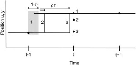
Integrating-detector model; three realizations of a step occurring between t and t+1 result in three different observed positions y_t (solid circles). If the step occurs during the deadtime (instance 1; corresponds to ρ = 0 in Eq. 1) the observed position at time t will reflect the full size of the step. Steps occurring after the deadtime (instances 2 and 3) result in smaller observed position changes, according to the variable τ in Eq. 1).

Based on this representation of the measured value, we can redefine the emission probability of the HMM (see Eq. 5 of (3)) as the probability density b_t(y_t, u_t−1, u_t) of y_t given the model λ and the true positions u_t and u_t−1 at that time and at the previous time point.

Let us define the reduced deviation

$${\upsilon }_{t,t^{\prime }}=\left(y_t-h\left(t\right)-u_{t^{\prime }}\right)/\sqrt{2}{\sigma }_t,$$

where h(t) is a function representing the baseline drift, and σ²_t is, as before, the time-dependent variance computed according to σ²_t = σ²₀ I₀/I_t. Here, σ₀ is a parameter to be determined, the nominal standard deviation; I₀ is the maximum reporter fluorescence intensity in the recording; and I_t is the intensity during the measurement for time point, respectively. The emission probability is then given by

$$b_t\left(y_t,u_{t-1},u_t\right)=\{\begin{array}{ll}{\left(\sqrt{2\pi }{\sigma }_t\right)}^{-1}\exp \left(-{\upsilon }_{t,t}^2\right),\hfill & u_{t-1}=u_t\hfill \\ \frac{1-\eta }{\sqrt{2\pi }{\sigma }_t}\exp \left({\upsilon }_{t,t}^2\right)+\frac{\eta }{2\left(u_{t-1}-u_t\right)}\left[\text{erf}\left({\upsilon }_{t,t-1}\right)-\text{erf}\left({\upsilon }_{t,t}\right)\right],\hfill & \text{otherwise}\hfill \end{array}.$$ (2)

This new form for b defines the integrating detector version of our algorithm, denoted VSI-HMM. In the previous article (3), b was simply a Gaussian probability density with mean u_t. The addition of a third argument, the true position of the motor at the previous time point, results in small changes to the forward-backward and reestimation algorithms. For example, the calculation of the forward variables α_i, described in Eqs. 9–11 of Müllner et al. (3), is now carried out as follows. Initialization is based on the assumption that the motor position has remained constant over the previous time step,

$${\alpha }_1\left(i,u\right)={\pi }_{iu}{b}_1\left(y_1,u,u\right)$$

and the recursion formula is

$${\alpha }_{t+1}\left(j,v\right)=\sum _{i=1}^n\sum _{u=1}^m{\alpha }_t\left(i,u\right)c_{ij}\left(v-u\right)b_{t+1}\left(y_{t+1},u,v\right),t=1,2,\dots T.$$ (3)

The likelihood is obtained, as before, from the final α-value as

$$P\left(Y|\lambda \right)=\sum _{i,u}{\alpha }_T\left(i,u\right).$$

It can be seen that the number of terms in the sums of Eq. 3 is unchanged, and the computational intensity is increased only by a small constant factor. However, the acceleration of the computation of the forward variables through the use of fast Fourier transforms is no longer possible. The same holds for the computation of the backward variables β_t and the reestimation variables γ_t and ξ_i (see Eqs. 17–19 of (3)). In addition to the changes in these calculations, a straightforward change was also made to the Viterbi algorithm to incorporate the new form of the b function.

MAP estimation of transition probabilities

Let λ = (τ, C, σ₀) be the parameters of the VSI-HMM which are to be optimized: π is a vector of the initial probabilities, C is the matrix of transition probabilities c_ij(w), and σ₀ is the noise parameter. The likelihood, L, is defined to be the probability P(Y|λ) of the observed data sequence Y = y₁, y₂, …, y_T, given the model.

Maximum a posteriori (MAP) estimation is an extension of the maximum likelihood (ML) method in which prior information, in the form of a prior probability function P(λ), conveys knowledge about the likely values of model parameters. Where ML estimation maximizes the likelihood P(Y|λ), MAP estimation maximizes the posterior probability P(λ|Y) which is proportional to P(Y|λ)P(λ). It thus incorporates the prior information, available before the experimental data are considered, and provides an optimum posterior estimate after including the information from the experimental data. In practice, the effect of the prior is substantial only when the information provided by the data Y is meager.

Consider the model parameter c_ij(0), which is the probability of remaining in the state i and making no position change during a single time step. For simplicity, we will use c_i in this section as a shorthand for c_ii(0). Chemical rate theory says that, although the dwell time is an exponentially distributed random variable, its mean value τ_d = 1/(1−c_i) is, in turn, an exponential function of the activation energy. The application of classical ML estimation implicitly assumes that all values of the c_i parameter between zero and one are equally likely. Thereby, one implicitly assumes that the activation energy E is distributed ∝ e ^−E/kT with the system's thermal energy given by kT; that is, large activation energies are exponentially less common than smaller ones. From the very broad range of mean dwell-times observed in single-molecule experiments such as single-ion-channel recordings, the uniformity assumption for c_i appears not to be valid. Guided by this prior knowledge, we assume instead that activation energies are taken from a uniform distribution. In this case, the mean dwell time τ_d = 1/(1−c_i) will have a probability density proportional to 1/τ_d, and c_i will have the prior probability density

$$p\left(c_i\right)\propto \frac{1}{1-c_i}.$$

This prior probability density ensures that values of c_i between 0.9 and 0.91 (mean dwell times of 10 and 11 units) are assumed a priori to be as likely as values between 0.99 and 0.991 (dwell times of 100 and 110 units), and mean dwell times will be exponentially distributed. Unfortunately, this function is unbounded as c_i → 1. We therefore include a parameter ɛ, representing the lowest expected transition probability out of state i, to obtain

$$p\left(c_i\right)\propto \frac{1}{1-c_i+\varepsilon }.$$ (4)

In the simulations described in this article the choice of ɛ had little influence on the results; we conclude that a very rough estimate is sufficient. If truly no information about mean dwell times is available, one choice for its value could be 0.7/T, corresponding to a 0.5 probability that at least one transition out of state i would occur within the entire observation period.

The maximization of the posterior probability P(Y|λ)P(λ) can be carried out using the E-M algorithm. The prior probability densities are denoted p(c_i) for i = 1…, n. Maximization of the Q function of the E-M iteration under the constraints that

$$\sum _{j,w}{c}_{ij}\left(w\right)=1$$

yields equations for the k+1^st estimates of the c_i,

$$c_i\sum _{\left\{j,w\right\}\ne \left\{i,0\right\}}\sum _{t=1}^{T-1}{\xi }_t^{\left(k\right)}\left(i,j,w\right)+\left(c_i-1\right)\sum _{t=1}^{T-1}{\xi }_t^{\left(k\right)}\left(i,i,0\right)+c_i\left(c_i-1\right)\frac{d\ln p\left(c_i\right)}{d{c}_i}=0,$$ (5)

where x_t (i,j,w) is the probability of making a transition at time t from molecular state i to j with a step of size w, given the data Y and the model λ. The remaining c_ij(w) are obtained as

$$c_{ij}^{\left(k+1\right)}\left(w\right)=\frac{\sum _{t=1}^{T-1}{\xi }_t^{\left(k\right)}\left(i,j,w\right)}{\sum _{\left\{h,w\right\}\ne \left\{i,0\right\}}\sum _{t=1}^{T-1}{\xi }_t^{\left(k\right)}\left(i,h,w\right)}\left(1-c_i^{\left(k+1\right)}\right).$$ (6)

The reestimation formulas in Eqs. 5 and 6 generally hold for all prior probability densities which fulfill minimal requirements (differentiability and boundedness on [0,1]). Note that for uniformly distributed c_i, Eqs. 5 and 6 are identical to Eq. 22 of Müllner et al. (3), the classical ML estimation formula. We employed MAP estimation in the comparisons with step detectors in Figs. 2 and 3, with the prior probability Eq. 4 for p(c_i) and the parameter value ɛ = 0.005 chosen to model a maximum expected dwell time of ∼200 time points. As it turned out, however, the inclusion of the prior probability densities made very little difference to the results of these simulations.

Figure 2.

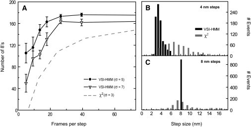
Comparison of the performance of the VSI-HMM-Viterbi algorithm with the χ² detector of Kerssemakers et al. (6). (A) Motor time courses, each containing 200 steps of size 8 nm with mean dwells of 24 points, were generated using the continuous-time simulator. From the HMM-Viterbi restorations the Number of 8's metric of Carter et al. (1) was evaluated and plotted. This metric counts the number of detected steps that occur at the correct time (±2 sample intervals) and have the correct size (8 ± 3 nm); error bars indicate the standard deviations from 10 trials at each mean step duration. The performance with root mean square noise levels of 5 and 7 nm (circles and triangles) was superior to that from the filtered χ² detector even at the lower noise level of 3 nm (dashed line, data from Fig. 6 of (1)). MAP estimation with ɛ = 0.001 was employed, although indistinguishable results were obtained with ɛ = 1, that is with essentially no effect from the MAP prior probability. (B) Steps recovered by VSI-HMM-Viterbi from 18 simulations, each with σ = 6 nm and comprised of 50 steps of size 4 nm. Even at the large noise level, the small steps are detected with high accuracy: mean = 3.6 nm, standard deviation = 2 nm. The χ² detector finds a broader distribution of step sizes that extends beyond 8 nm. (C) Same as in panel B but with all simulated steps 8 nm in size. The steps were detected with almost no error. In comparison, the χ² method found a broad range of step sizes. In panels B and C, the simulation assumed a mean velocity of 300 nm/s and a frame rate of 2000 s^–1; MAP estimation was employed, with ɛ = 0.005, and the ${\chi }^2$ detector data are from Fig. 8c and 8d of Carter et al. (1).

Figure 3.

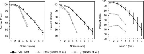
Further evaluation of the VSI-HMM-Viterbi reconstruction (▪) of a simulated stepping time-course. These data are compared with the results of simulations using χ²(▾), and t-test (▴) detectors with optimized filters as reported by Carter et al. (1). The three metrics of Carter et al. (1) are shown: panel A plots the fraction of actual steps that are detected (that is, the fraction of true positives); panel B plots the fraction of the detected steps that correspond to actual ones (that is, unity minus the fraction of false positives); and panel C shows the percentage of 8 nm (±3 nm) steps in the population of true positive events. The task assigned to each step detection method was to interpret simulations having 200 steps of size 8 nm and mean dwell time of 24 points. This was repeated multiple times for each value of added Gaussian noise. Error bars on the HMM data are standard deviations of the respective results from 20 different simulations. Data for the t-test and χ² are taken from Fig. 5 of Carter et al. (1). The HMM algorithm performs better than the other methods in all three metrics, in particular when noise is large.

Baseline drift

It is also possible to estimate parameters describing a drifting baseline. We model the baseline drift as a piecewise-linear function, as was done in Venkataramanan and Sigworth (4). Let the T sample points be divided into R segments, each Δ = T/R points long. Defining a set of triangular-pulse functions

$$h_r\left(t\right)=\max \left(1-\frac{\left|t-r\Delta \right|}{\Delta },0\right),$$

$$r=0\dots ,R,$$

the baseline function can be expressed in terms of the R+1 vertex values κ_r,

$$h\left(t\right)=\sum _{r=0}^R{\kappa }_r{h}_r\left(t\right).$$ (7)

The E-M reestimation of the vertex values is equivalent to a weighted least-squares problem expressed by

$$\Omega \kappa =\Gamma ,$$ (8)

where the matrix Ω and vector Γ are given by

$${\Omega }_{rs}=\sum _t{h}_r\left(t\right)h_s\left(t\right)/{\sigma }_t^2$$

and

$${\Gamma }_r=\sum _t{h}_r\left(t\right)\left(y_t-\sum _{i,u}u{\gamma }_t\left(i,u\right)\right)/{\sigma }_t^2.$$

The process of baseline reestimation is carried out as follows. At the k^th iteration, the set of vertices κ_r^(k) is used to compute the baseline function according to Eq. 7, and this function is used to evaluate the emission probability (see Eq. 2) and, through the forward-backward algorithm, the state probabilities γ_t⁽ⁱ⁾(i,u) (Eq. 18 of (3)). Equation 8 is then solved to yield the new set of vertices κ_r^(k+1).

Simulation

Simulations of stepping time courses in this article were created with a continuous-time simulator based on the Gillespie algorithm (5). Dwell times are obtained as exponentially distributed random numbers, and the times of stepping events are not assumed to be synchronized with the sampling times. The sampled position is therefore the output of a boxcar filter with the integration time equal to η, so that detector integration is accurately modeled. Unless noted, both the simulation and the analysis employed η = 1. To each position value, a Gaussian random number is added to emulate the measurement noise.

As in the algorithms described in the previous article (3), the simulator and VSI-HMM algorithms were implemented using MATLAB, in functions named StepSimulatorC.m, ForwardBackward_3.m, and ViterbiRestoration.m. This code and example scripts can be found at The MathWorks File Exchange site, www.mathworks.com/matlabcentral/fileexchange/24697.

Results

Recently, Carter et al. (1) assessed the strengths and weaknesses of a number of step-detecting methods currently available to analyze noisy motor-protein recordings. The authors defined three performance metrics to allow evaluation of the performance of several algorithms; the χ² detector of Kerssemakers et al. (6) performed the best overall. Here, we compare performance of the VSI-HMM with that of the χ² step detector.

To use HMM signal processing as a step detector, ML or MAP estimation must first be applied to optimize the parameters of the hidden Markov model. These parameters are the step-size distributions and transition probabilities. For the tests shown here we used the one-state HMM, which models the very simple kinetics of Poisson-distributed dwell times. In the analysis, the starting parameter values corresponded to a uniform distribution of step sizes over the range of −32 to 32 nm, and a mean dwell time of 10 points. After 100 iterations, the model was deemed to have converged; at this point the model parameters, along with the original simulated time course, were fed to the Viterbi reestimation algorithm to provide a restoration of the noiseless time course.

Fig. 2 A shows as a performance metric the fraction of steps found to have the correct amplitude (8 ± 3 nm) from a simulation containing 200 steps with mean dwell time of 48 points. By this metric, the VSI-HMM-Viterbi idealization performs better at all values of the mean dwell time. For example, when the data have a noise standard deviation σ = 7 nm, the VSI-HMM-Viterbi method yields better results than the χ² detector does when the noise is only σ= 3 nm. Carter et al. (1) also compared the ability of step detectors to identify steps of 4 or 8 nm, with dwells of 27 or 53 time points, respectively, in the presence of noise having σ = 6 nm. VSI-HMM-Viterbi restorations of these trajectories (Fig. 2, B and C) show narrow distributions of step sizes with mean values of 3.6 and 8 nm. In contrast, the χ² detector found very broad distributions (0.5–17.5 nm) in both cases and failed to find a peak near 4 nm.

In Fig. 3, three more comparisons are made between the VSI-HMM-Viterbi step detector and the detectors examined by Carter et al. (1), as the noise level is changed. In every case the HMM analysis is greatly superior to the step detectors. Indeed, roughly equivalent levels of detection fidelity are obtained at nearly twice the noise level with the HMM detection scheme.

The VSI-HMM algorithm explicitly accounts for the intermediate data points that result inevitably from the detector's integration during a tracking experiment. Fig. 4 A shows part of a 500-datapoint simulation with large 64-nm steps alternating with short steps randomly picked (with equal probability) to be 20 or 10 nm in size, as used previously ((3), Fig. 1 D). The simulation included the effect of the detector integration time with a duty cycle η = 1; consequently, an intermediate position value resulted whenever a step was taken. Despite the large noise and the intermediate data points, the Viterbi restoration based on the proper HMM with η = 1 (Fig. 4 B) reproduced the steps accurately. These data were also analyzed with the simpler VS-HMM (Fig. 4 C) in which intermediate position values are not modeled (η = 0). Unable to differentiate between an actual transition and a position point corresponding to the molecule being in transit, the simplified HMM finds kinetic events with steps of various sizes that differ from the true 64-, 20-, and 10-nm steps (inset of Fig. 4 C).

Figure 4.

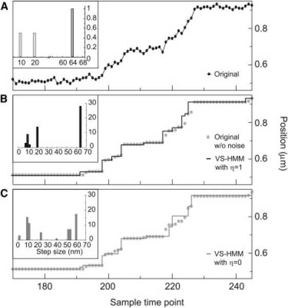
Analysis of a recording with intermediate points. (A) Portion of a stepping time-course from the continuous-time simulator. The kinetics, step sizes (see inset histogram), and noise level (7 nm) are identical to those in Figs. 1 and 2 of the previous article (3); however, now the simulation includes the effect of detector integration time, with duty cycle η = 1. (B) Analysis based on the VSI-HMM which includes the integration effects withη = 1. The Viterbi restoration (solid line) is compared with ground truth, that is the original simulation without noise (circles). Steps are identified accurately despite the presence of intermediate points as identified in the histogram of restored step sizes shown in the inset. Parameters of the VSI-HMM analysis were T = 500, n = 2, and m = 190, with the quantum of position being 1 nm; each iteration required 3.4 s on a 2 GHz processor and convergence was complete after 100 iterations. (C) Analysis with the nonintegrating VS-HMM. Due to the FFT speed-up, the VS-HMM required only 0.6 s per iteration, but it did not reliably distinguish the two populations of small steps. The restoration (solid line) has large errors and the histogram of restored step sizes (inset) shows spurious step sizes.

The simulation in Fig. 4 B also serves as a test of the application of the VSI-HMM, fundamentally a discrete-time algorithm, to the simulated continuous-time stepping process. One of the mean dwell times in the simulated data was only five time points, which might be expected to yield missed-event errors, as discussed in the preceding article (3). Nevertheless, the VSI-HMM obtained high-quality estimates for the step sizes and dwell times. In the analysis of 20 independent simulations, the estimates of the 10-, 20-, and 64-nm step sizes, taken as the center of mass of the peaks of the step-size distribution c_ij(w), were (mean ± SD): 10.8 ± 2.1, 21.1 ± 1.4, and 65.1 ± 1.2 nm. The mean dwell times were estimated (according to Eq. 2 of the preceding article (3)) to be 10.5 ± 1.9 and 5.8 ± 2.1 time points. These values are quite close to the simulated mean dwell times of 10 and 5 time points and the standard deviations are reasonable, particularly in view of the fact that the finite number of steps in a 500-point simulation, in itself, yields a sampling error of ∼17% in the mean dwell times.

Finally, we applied the HMM to actual experimental data obtained under demanding conditions. Fig. 5 A shows the recording of a myosin V motor tagged on a calmodulin site with a fluorescent dye. The myosin V walked in the presence of 300 nM ATP on actin in vitro while two orthogonally polarized beams alternately excited the dye molecule every 0.5 s (see Methods in (7)). Under these conditions, the emission showed strong fluctuations (Fig. 5 A, lower panel) as the motor protein switched between orientational states whereas translocating hand-over-hand on actin. Due to the intensity modulations, the noise variance was itself time-dependent. Application of a two-state VSI-HMM to the data (with η = 1 to match the CCD camera duty cycle) resulted in the restoration (red line) with alternating 64- and 10–12-nm steps. The deduced ATPase rate of 0.27 s⁻¹ is in very good agreement with that expected for myosin V given an ATP concentration of 300 nM (8). Although the 64-nm steps are straightforward to note by eye, several of the 10-nm steps are obscured due to noise. An analysis by eye would therefore have categorized the molecule as a 74-0-74 type stepper (9). However, by directing the Viterbi restoration along the points with low variance, the HMM analysis successfully uncovered the 64-10 nm pairs. Single myosin V recordings at lower ATP concentration and higher S/N do indeed support the HMM conclusion that in many cases the apparent 74-0 steppers are 64-10 types (7).

Figure 5.

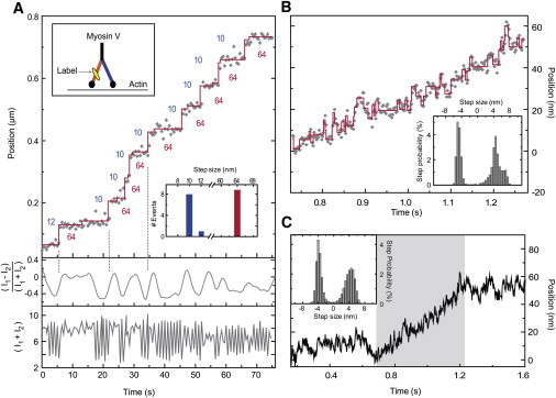
Applications of the HMM algorithm to experimental recordings. (A) Measured position (gray diamonds) of a processive myosin-V motor labeled on the calmodulin site closest to its motor domain (upper inset). HMM analysis and restoration (solid staircase and inset histogram) reveal alternating 64-nm and 10-nm steps. Imaging with alternating orthogonal excitation polarizations (see (7)) produced large modulations in the emission intensity (bottom panel) as the motor protein underwent conformational changes. The intensity data were incorporated into the noise model. Polarization changes, indicated by differences in intensity between successive frames (middle panel) accompany steps as found in the Viterbi restoration; three such steps are marked with vertical dashed lines. (B) Position data obtained from bright-field illumination of a melanosome being transported in vivo. Viterbi restoration (solid staircase) shows bidirectional stepping, presumably forward due to kinesin 2 and backward due to dynein. The MAP-estimated step size distribution (inset) indicates the majority of steps to be ∼5 nm in size, and not 8 nm. The data show an overall positive slope, but reveals a large number of backward steps. In the Viterbi reconstruction, there are 32 forward and 24 backward steps. (C) A longer stretch of the same recording. Outside of the portion shown in panel B (shaded region) there are almost equal numbers of forward and backward steps, suggesting an even stronger tug-of-war among the microtubule-binding motor proteins.

Fig. 5, B and C, shows a recording of a Xenopus melanophore melanosome being transported by the motor proteins cytoplasmic dynein and kinesin 2 in vivo (10). Here, we define increasing position as movement away from the cell nucleus (anterograde). Melanosome images were captured with bright-field illumination every 2 ms. Small step size, high rate of ATP turnover, and large instrumentation noise at this acquisition rate, make the recording difficult to interpret by eye. Fig. 5 B shows a 540-ms stretch of the recording during which the melanosome is apparently moving steadily away from the nucleus. Analysis with a one-state HMM, however, revealed both retrograde and anterograde steps in this recording, as well as in the full 1.5 s recording shown in Fig. 5 C, indicating the presence of dynein and kinesin. In both cases the step-size distributions peaked at ±4–5 nm (see insets) and not ∼8 nm in size, as expected from single kinesin or dynein tracks (11,12).

In the estimated distribution of step sizes for Fig. 5 B, the fraction of positive steps larger than 7 nm was <5%. In the longer recording in Fig. 5 C, this fraction was <2%. The small steps are most likely a consequence of multiple motors interacting with the same cargo. This in vivo result is consistent with the recent in vitro gliding assays results of Leduc et al. (13). That the retrograde movements are largely due to dynein, and not kinesin-2 switching between backward and forward steps, is deduced from the fact that the intracellular drag force on a ∼600-nm load moving ∼100 nm/s is < 5 pN (14), smaller than forces where kinesin bidirectional stepping becomes dominant (15).

How can one assess the level of certainty of concluding that there are negatively-directed movements, or that there are stepwise movements at all?

This can be done by comparing log likelihood values. When, in the model, the steps were restricted to only positive values, the log Likelihood L dropped by 40 units, a highly significant decrease corresponding to a likelihood ratio of e^–40 ≈ 10⁻¹⁷. Further, constraining step sizes to be outside the range of –4 nm to +7 nm caused L to decrease by 83 units, strongly indicating the presence of steps ≤7 nm in size. That the data represent stepwise movement and not just a drift was verified by fitting with a model in which there were no steps at all, but just a linear baseline drift plus white noise. In this case the likelihood decreased by 94 units. Furthermore, the steps are likely not to be artifacts of the detection system, because they were observed in several cases when the sample interval was varied between 1 and 2.5 ms.

We also applied the VSI-HMM analysis to synthetic timecourses with similar statistics (see Fig. S1 in the Supporting Material). The combination of a linear ramp and white noise yields, as expected in the HMM analysis, a rapid succession of minimal-sized steps. On the other hand, analysis of a combination of a linear ramp and Lorentzian noise yields positive and negative steps ∼4 nm in size. This example illustrates that the results of the analysis are based on the model assumption—that discrete steps underlie the motor motion—and that application of the analysis to inappropriate datasets can attain misleading results. Nevertheless, we conclude that the underlying events in Fig. 5 B are clearly smaller than 8 nm in magnitude.

Previous analyses of intracellular transport have focused exclusively on high S/N portions of long trajectories that are readily interpretable by eye. This raises the possibility of an observer bias in favor of large steps, ∼8 nm in magnitude (such as in Fig. S2), with the observer avoiding recordings of tugs-of-war between different motors or multiple motors pulling in the same direction (16,17). The new VSI-HMM method allows better investigation of typically noisy in vivo recordings. In this instance, HMM analysis of a single melanosome transport shows that in living cells there are cases where uncoordinated ATPase activity of several motors can, in fact, lead to ∼±4–5 nm steps. This is most readily explained by two kinesins (+ direction), or two dyneins (− direction) pulling on the cargo in a noncooperative manner (13). It is also possible that there is a tug-of-war between kinesin(s) and dynein(s).

Discussion

The new algorithm offers several advantages over existing strategies. In terms of simple step detection, the method yields more accurate results than the current state-of-the-art techniques (Figs. 2 and 3). Compared to currently available Markov-model based methods (2,18), the VSI-HMM is quite insensitive to the choice of initial model parameters, making it an effectively automatic algorithm for interpreting poor S/N recordings (see also (3)).

Additionally, the VSI-HMM includes three critical technical advances:

First, the VSI-HMM explicitly handles the experimentally unavoidable intermediate points that arise from the finite integration time of the detector. Large errors can appear in interpretation if the analysis method is unable to account for the points, and we have shown how the new method rectifies this problem (Fig. 4).

Second, the VSI-HMM method directly accommodates time-varying noise due to large variations in photon flux from single fluorescent reporters (Fig. 5 A and Fig. S2 A) or absorbance reporters (Fig. 5 B).

Third, the implicit assumption of uniformly distributed dwell times can be corrected by incorporating the model in a MAP framework.

Owing to the inherent confusion in interpreting noisy recordings by eye, conclusions from single-molecule experiments are often limited by data quality. In the case of in vitro stepping data, the HMM clearly shows that myosin V motors previously thought to show 74 nm and 0 nm are in fact 64-10 nm walkers; when their time courses are fitted by eye, one easily misses the small steps (9). Although previous HMM analyses find small steps if the hypothesis of small steps is tested explicitly (18), the improved method presented here can automatically uncover their presence. Interpretation of in vivo data is another such example, where a lack of sophisticated methods has been restricting the level of details that could be derived from high-resolution traces.

Here we have shown how the new, robust VSI-HMM approach permits wholesale dissection of long and noisy transport data. Our HMM analysis has revealed that there are bidirectional steps, a large fraction of which are smaller than 8 nm in size, from an in vivo recording of melanosome transport. This establishes that more than one kinesin or dynein are involved in intracellular cargo transport, a subject of considerable controversy (19), although how they cooperate or compete remains an open question. Approaches such as the one presented here provide rapid and unbiased ways of analyzing difficult results and its availability should provide an alternative way to circumvent some of the constraints currently hindering single-molecule experiments.

References

- 1.Carter B.C., Vershinin M., Gross S.P. A comparison of step-detection methods: how well can you do? Biophys. J. 2008;94:306–319. doi: 10.1529/biophysj.107.110601. [DOI] [PMC free article] [PubMed] [Google Scholar]
- 2.Milescu L.S., Yildiz A., Sachs F. Maximum likelihood estimation of molecular motor kinetics from staircase dwell-time sequences. Biophys. J. 2006;91:1156–1168. doi: 10.1529/biophysj.105.079541. [DOI] [PMC free article] [PubMed] [Google Scholar]
- 3.Müllner F.E., Syed S., Sigworth F.J. Improved hidden Markov models for molecular motors, part 1: basic theory. Biophys. J. 2010;99:3684–3695. doi: 10.1016/j.bpj.2010.09.067. [DOI] [PMC free article] [PubMed] [Google Scholar]
- 4.Venkataramanan L., Sigworth F.J. Applying hidden Markov models to the analysis of single ion channel activity. Biophys. J. 2002;82:1930–1942. doi: 10.1016/S0006-3495(02)75542-2. [DOI] [PMC free article] [PubMed] [Google Scholar]
- 5.Gillespie D.T. Exact stochastic simulation of coupled chemical reactions. J. Phys. Chem. 1977;81:2340–2361. [Google Scholar]
- 6.Kerssemakers J.W., Munteanu E.L., Dogterom M. Assembly dynamics of microtubules at molecular resolution. Nature. 2006;442:709–712. doi: 10.1038/nature04928. [DOI] [PubMed] [Google Scholar]
- 7.Syed S., Snyder G.E., Goldman Y.E. Adaptability of myosin V studied by simultaneous detection of position and orientation. EMBO J. 2006;25:1795–1803. doi: 10.1038/sj.emboj.7601060. [DOI] [PMC free article] [PubMed] [Google Scholar]
- 8.Rief M., Rock R.S., Spudich J.A. Myosin-V stepping kinetics: a molecular model for processivity. Proc. Natl. Acad. Sci. USA. 2000;97:9482–9486. doi: 10.1073/pnas.97.17.9482. [DOI] [PMC free article] [PubMed] [Google Scholar]
- 9.Yildiz A., Selvin P.R. Fluorescence imaging with one nanometer accuracy: application to molecular motors. Acc. Chem. Res. 2005;38:574–582. doi: 10.1021/ar040136s. [DOI] [PubMed] [Google Scholar]
- 10.Kural C., Serpinskaya A.S., Selvin P.R. Tracking melanosomes inside a cell to study molecular motors and their interaction. Proc. Natl. Acad. Sci. USA. 2007;104:5378–5382. doi: 10.1073/pnas.0700145104. [DOI] [PMC free article] [PubMed] [Google Scholar]
- 11.Reck-Peterson S.L., Yildiz A., Vale R.D. Single-molecule analysis of dynein processivity and stepping behavior. Cell. 2006;126:335–348. doi: 10.1016/j.cell.2006.05.046. [DOI] [PMC free article] [PubMed] [Google Scholar]
- 12.Schnitzer M.J., Block S.M. Kinesin hydrolyses one ATP per 8-nm step. Nature. 1997;388:386–390. doi: 10.1038/41111. [DOI] [PubMed] [Google Scholar]
- 13.Leduc C., Ruhnow F., Diez S. Detection of fractional steps in cargo movement by the collective operation of kinesin-1 motors. Proc. Natl. Acad. Sci. USA. 2007;104:10847–10852. doi: 10.1073/pnas.0701864104. [DOI] [PMC free article] [PubMed] [Google Scholar]
- 14.Hill D.B., Plaza M.J., Holzwarth G. Fast vesicle transport in PC12 neurites: velocities and forces. Eur. Biophys. J. 2004;33:623–632. doi: 10.1007/s00249-004-0403-6. [DOI] [PubMed] [Google Scholar]
- 15.Carter N.J., Cross R.A. Mechanics of the kinesin step. Nature. 2005;435:308–312. doi: 10.1038/nature03528. [DOI] [PubMed] [Google Scholar]
- 16.Kural C., Kim H., Selvin P.R. Kinesin and dynein move a peroxisome in vivo: a tug-of-war or coordinated movement? Science. 2005;308:1469–1472. doi: 10.1126/science.1108408. [DOI] [PubMed] [Google Scholar]
- 17.Nan X., Sims P.A., Xie X.S. Observation of individual microtubule motor steps in living cells with endocytosed quantum dots. J. Phys. Chem. B. 2005;109:24220–24224. doi: 10.1021/jp056360w. [DOI] [PubMed] [Google Scholar]
- 18.Milescu L.S., Yildiz A., Sachs F. Extracting dwell time sequences from processive molecular motor data. Biophys. J. 2006;91:3135–3150. doi: 10.1529/biophysj.105.079517. [DOI] [PMC free article] [PubMed] [Google Scholar]
- 19.Gross S.P., Vershinin M., Shubeita G.T. Cargo transport: two motors are sometimes better than one. Curr. Biol. 2007;17:R478–R486. doi: 10.1016/j.cub.2007.04.025. [DOI] [PubMed] [Google Scholar]
Associated Data
This section collects any data citations, data availability statements, or supplementary materials included in this article.