Relation between temperature and suicide mortality in Japan in the presence of other confounding factors using time-series analysis with a semiparametric approach

Abstract

Objectives

The objective of this study was to assess the relation between temperature and suicide mortality in Japan using time series analysis with a semiparametric approach.

Methods

We analyzed the relation between daily fluctuations in suicide mortality and maximum temperatures for all regions in Japan over the period of time from 1972 to 1995 using a generalized additive model. The model controls for the time trend, season, selected meteorological parameters, day of the week, and holiday. Adjustment was based using penalized splines and the decision on the amount of smoothness was based on minimizing the unbiased risk estimation criterion.

Results

The results show that suicide mortality in Japan has a seasonal character and it varies from year to year, with the highest occurrence in April, as well as in the first part of the week, especially on Mondays and Tuesdays. As for the day of the week, there were only few suicide cases on Saturdays and holidays. We found that for all regions in Japan when temperature increased the suicide mortality increased on the same day (lag = 0). Analysis by method of suicide showed that when temperature increased mortality significantly increased only for suicide by a violent method. The pattern of the relation for other methods remained unclear.

Conclusions

This study suggests that an increase in temperature has a short-term effect on suicide mortality in Japan.

Introduction

The suicide mortality in Japan is one of the highest in industrialized countries and it has been associated with a range of factors, such as changes in socioeconomic conditions [1], alcohol consumption [2], a rare psychiatric disorder called folie à deux [3], the internet [4–6], and factors obtained from psychological autopsies [7].

There are large numbers of studies on seasonal variations in suicide mortality, with the most common peak occurring in late spring or early summer [8–13]. The seasonality of suicide in Japan was explored by Sato [14], who examined monthly data using harmonic analysis to identify seasonal components in the variation of monthly suicides; the analysis revealed that more than 65% of the total variance in suicide was explained by the seasonal component. Another study evaluating the risk of suicide found that, although there was a seasonal pattern in deaths, after controlling for the seasonal confounders, there was a short-term association between daily temperature and suicide [15].

Many studies have identified significant relations between suicide and meteorological variables [8, 9, 11–13, 16, 17] and some have found that there are no associations between meteorological variables and suicide [18–22]. Furthermore, it has been shown that the effect of high temperatures on suicide will probably become more important as global warming continues [23].

A variety of statistical techniques can be used to examine the relation between weather and suicide. In this study, to assess the relation between temperature and suicide mortality in Japan, we used one of the time series analyses with a semiparametric statistical approach [24–26], a generalized additive model (GAM) [25] with penalized splines [27], as this approach provides sufficient flexibility in capturing the trend and seasonality of the time series [28, 29].

Materials and methods

Data

All data (47 prefectures of Japan) on daily suicide deaths, classified as ‘non-violent’ (ICD-9: E950.0–E952.9; ICD-10: X60–X69) and ‘violent’ (ICD-9: E953.0–E958.9; ICD-10: X70–X84) methods, as well as deaths from accidents (ICD-9: E800.0–928.0; ICD-10: V01–V99, W01–W99, X01–X59) and homicides (ICD-9: E960.0–969.0; ICD-10: X85–X99, Y01–Y09), were provided by the Ministry of Health and Welfare of Japan. These data are classified by gender, age, year, and area code and were obtained for the 24-year period from 1972 to 1995, except for Okinawa, where the period was from 1973 to 1995. The population data were provided by the Prime Minister’s Office of Japan. The corresponding meteorological data, including the maximum, minimum, and average temperatures, relative humidity, atmospheric pressure, and sunshine duration, were provided by the Japan Meteorological Agency (JMA).

The daily maximum temperature of the capital city of a prefecture was used as an exposure variable. When data were not available for the capital city, those for the closest city with an observatory station were used instead.

Because of the relatively small number of suicide deaths on individual days, the data from 47 prefectures were merged into 9 geographical regions.

Analysis and methods

In general, in time series analysis there is complexity of the confounders, such as seasonal and long-term trends. In estimating the effect of temperature on mortality using time series analysis, it is necessary to control for potential confounders, which vary on time scales similar to those for the response variables [29].

We used a special type of semiparametric Poisson regression, GAM [30], assuming that the observed suicide deaths are Poisson random variables, although the computed variance–mean ratios were slightly greater than one:

1

where Y_t is the suicide mortality count for day t; μ_t is the expected suicide mortality for day t; x_t is the maximum temperature on day t; f is a smooth function of time (t); v_t represents observed time-varying variables such as relative humidity, atmospheric pressure, and sunshine duration; s is a smooth function of variables x_t and v_t; h_t is a linear term for a holiday indicator (0–1); and w_t is the day of the week indicator (0–6); ε_t ~ N(0, σ²), where σ² > 0.

We used a penalized spline function as a basis to represent the smooth function and specified an appropriate amount of smoothness to account for the penalization [29].

Then the model takes the form:

where suicide_i ~ Poisson (link = log),

f

Smooth function of time;

tmax_t

Maximum temperature on day i;

s_i

Smooth functions of measured time-varying confounders, such as

pst_i

Atmospheric pressure,

rhum_i

Relative humidity,

sun_i

Sunshine duration,

dow_i

Factor variable of the day of the week (0–6), and

hol_i

Factor variable of a holiday (0–1)

The smoothness of the time function is controlled by a smoothing parameter, or degree of freedom (df), which, in this study, was estimated by minimizing the unbiased risk estimation (UBRE) criteria [31].

To fit the model we used the gam function from the {mgcv} package in R statistical software, version 2.6.2 [32], which is available through the Comprehensive R Archive Network (CRAN) mirror site (http://cran.r-project.org/).

Once the best-fitted model had been selected, we then tested for overdispersion using the overdispersion parameter, and for residual autocorrelation using the simple (ACF) and partial autocorrelation function (PACF) plots.

Overdispersion

When working with Poisson errors, overdispersion can be a problem. It can occur because one or more of the important factors have not been measured. It may also result from the underlying distribution being non-Poisson. In the worst case this means that all of the predictor variables that were measured might be unimportant [33]. One general technique available to deal with this problem is to use a quasi-likelihood method by specifying the variance function instead of giving a full probability model: (general form for Poisson distribution), where φ is the dispersion parameter [34]. When φ > 1 there is an overdispersion.

R has a family quasipoisson in GAM to handle this situation.

Autocorrelation

Randomness is one of the key assumptions in determining whether a univariate statistical process is in control. This randomness is ascertained by computing autocorrelations for data values at varying time lags. Our data were assumed to be random when such autocorrelations were near-zero for any and all time-lag separations.

Results

The suicide deaths, rates, and the means by region (from north to south) for the study period from 1972 to 1995 are represented in Table 1.

Table 1.

Descriptive statistics of analysis variables (period of study from 1972 to 1995, Japan)

N	Region	Death count	MRa	Mean	Tmaxb (°C)	Rhumc (%)	Pstd (hPa)	Sune (h)
1	Hokkaido	24489	0.5	2.79	12.6	70.2	1010.3	5.4
2	Tohoku	47548	0.57	5.42	15.7	72.9	1005.4	5.0
3	Kanto	134284	0.43	15.32	19.1	68.0	1007.3	5.6
4	Chubu	87744	0.49	10.01	18.9	70.9	1003.5	5.4
5	Kinki	89250	0.47	10.18	19.9	69.0	1008.7	5.6
6	Chugoku	34803	0.52	3.97	19.7	73.5	1012.9	5.4
7	Shikoku	19902	0.55	2.27	20.5	68.3	1013.3	5.9
8	Kyushu	59383	0.52	6.77	21.2	72.0	1013.2	5.6
9	Okinawaf	4547	0.47	0.54	25.3	75.7	1009.3	5.5

The highest suicide mortality was observed in the Tohoku region (0.57) and the lowest in Kanto (0.43)

^aMortality rate

^bMaximum temperature

^cRelative humidity

^dStation level atmospheric pressure; hectopascal (hPa)

^eSunshine duration

^fThe period of the study was from 1973 to 1995

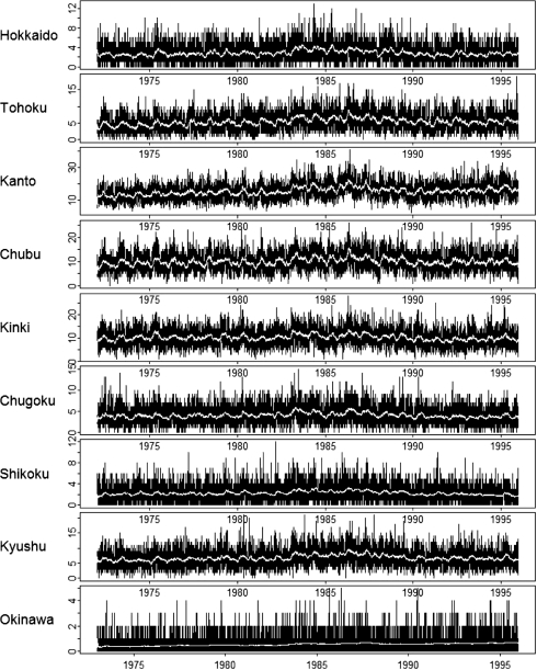
Figure 1 illustrates time-series of the suicide deaths in Japan by region. This crude data is difficult to analyze, although it is noticeable that the underlying deaths tend to vary with time.

Fig. 1.

Time-series and structural time-series of suicide mortality in Japan (1972–1995)

To estimate the effect of a 1° increase in temperature on the suicide deaths on a single day we used simple linear regression analysis and the results are shown in Table 2. It is noticeable that temperature affected suicide in most of the regions of Japan; however, the signal was low, probably due to the confounding of time trend and other seasonal factors, which have a strong relation with suicide mortality.

Table 2.

The estimated risk of suicide for each degree increase in temperature using simple linear regression analysis

Region	Risk estimate	Standard error	t value	Pr(>|t|)
Hokkaido	0.0219	0.0019	11.79	<2e−16***
Tohoku	0.0435	0.0029	14.96	<2e−16**
Kanto	0.0068	0.0063	1.09	0.2780
Chubu	0.0377	0.0043	8.70	<2e−16***
Kinki	0.0007	0.0044	0.16	0.8720
Chugoku	0.0113	0.0027	4.22	0.0000***
Shikoku	−0.0010	0.0021	−0.45	0.6530
Kyushu	0.0073	0.0039	1.86	0.0629†
Okinawa	0.0033	0.0016	2.00	0.0454*

The Pr(>|t|) is the p value for the slope: the probability of observing a t value this big or larger, if the null hypothesis (H0: slope = 0 is true). The t value is the value of Student's t for the slope = b/se_b. b is the slope, se_b is the standard error of the slope (b)

^†p = 0.1

* p = 0.05

** p = 0.01

*** p = 0.001

To obtain a better estimate of the relation between temperature and suicide, we tried to extract the temperature signal from the series by removing any seasonal and long-term trends in the data using a GAM model with smooth function of time.

The final model we obtained was as follows:

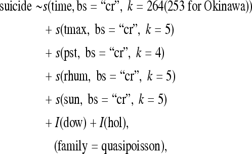where I is an indicator variable; bs is a smoothing basis built in to package mgcv; it is represented by cubic regression spline “cr”; k is the choice of dimension of the basis used to represent smooth terms.

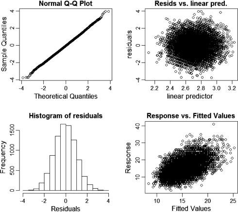
Basic model checking plots for the temperature–mortality model showed nothing problematic in the fitting of the relation (Fig. 2).

Fig. 2.

Basic residual plots for checking the generalized additive model (GAM) model fitting process (Kanto region). The upper left normal (Q-Q) plot is very close to a straight line, suggesting reasonable distributional assumption. The upper right plot suggests that variance is approximately constant as the mean increases. The histogram of residuals at the lower left appears consistent with normality. The lower right plot of response against fitted values shows a positive linear relation with a good deal of scatter: nothing problematic. Resids. residuals, pred. predictor, Q-Q Quantiles-Quantiles

The quasipoisson family was used in the GAM to deal with overdispersion:

 

Hokkaido	Tohoku	Kanto	Chubu	Kinki	Chugoku	Shikoku	Kyushu	Okinawa
1.15	1.08	1.08	1.06	1.06	1.07	1.17	1.06	1.03

Here we see that the overdispersion is tolerable.

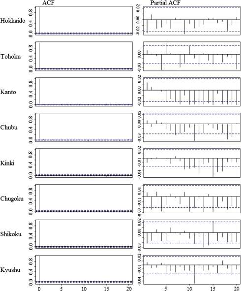
Autocorrelation plots of the residuals were checked to see whether the smooth terms sufficiently accounted for autocorrelation in the data, and the results suggested they almost did. After controlling for season and other confounding factors, the ACF and PACF of the suicide series showed no evidence of significant autocorrelation (Fig. 3). For all regions, the autocorrelation was mostly negative, implying that if a particular value is above average the next value (or for that matter the previous value) is more likely to be below average, and vice versa [35].

Fig. 3.

Autocorrelation and partial autocorrelation functions for the maximum temperature suicide model residuals obtained by GAM Poisson model. ACF autocorrelation function

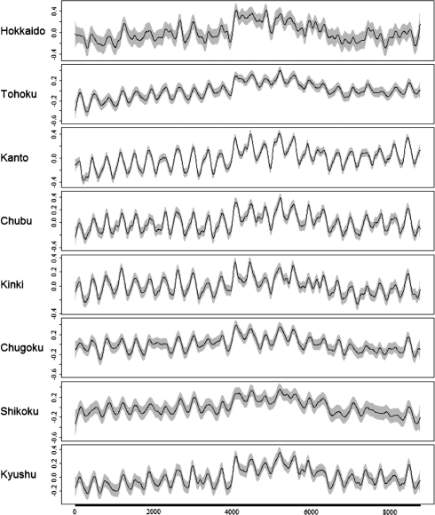
Figures 4, 5 and 6 illustrate estimates of the smooths from the model. Figure 4 shows the long-term trend in suicide deaths. A noticeable increase in the death rate occurred between the beginnings of the years 1983 and 1986 (on the figure this increase is approximately between 4000 and 5000 days from the 1st of January 1972).

Fig. 4.

The GAM-estimated effect of time component on suicide mortality for 8 regions in Japan (excluding Okinwa) (1972–1995). The continuous lines are the function estimates, and the shaded areas delimit the 95% confidence interval for the function. The numbers on each y-axis are the effective degrees of freedom of the term being plotted. The numbers on the x-axis indicate days starting from January 1st, 1972. Smoothing parameters are estimated by unbiased risk estimation (UBRE)/Akaike information criterion (AIC) [36]

Fig. 5.

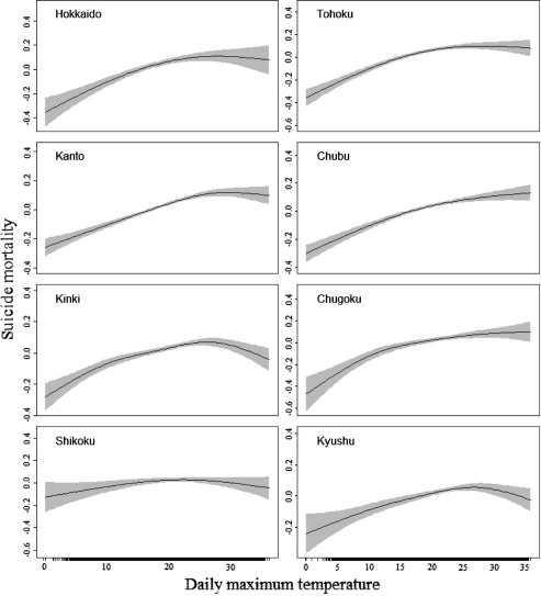
The GAM-estimated effect of maximum temperature (°C) on suicide mortality for 8 regions in Japan (excluding Okinawa). The continuous lines are the function estimates, and the shaded areas delimit the 95% confidence interval for the function. The numbers on each y-axis are the effective degrees of freedom of the term being plotted. Smoothing parameters are estimated by UBRE/AIC

Fig. 6.

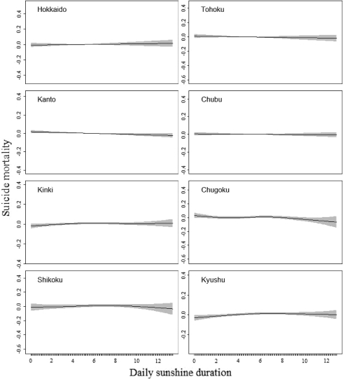
The GAM-estimated effect of sunshine duration (h) on suicide mortality for 8 regions in Japan (excluding Okinawa). The continuous lines are the function estimates, and the shaded areas delimit the 95% confidence interval for the function. The numbers on each y-axis are the effective degrees of freedom of the term being plotted. Smoothing parameters are estimated by UBRE/AIC

Figure 5 illustrates the short-term effect of temperature on suicide mortality. When the temperature increased the mortality increased for all regions, although the slopes of the curves tended to be lower for the southern regions. The confidence intervals are sufficiently narrow, suggesting that the curvature in the relation between suicide and temperature is real. Okinawa was the only region with no clear pattern of the relation, probably due to the small number of suicide deaths on the individual days (results are not shown).

In our study we could not obtain any significant effect of sunshine duration on suicide mortality (Fig. 6).

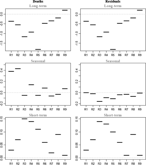
Figure 7 shows three different timescales, at which correlations between temperature and suicide deaths might be confounded by the hours of daylight. The left part of the figure shows the estimated correlation coefficients of suicide deaths on different timescales, and the right part represents the estimated correlations of the residuals taken after regressing the suicide deaths and temperature on the hours of daylight. For all regions, except Okinawa (R9), the long-term timescale was negatively correlated for both the suicide deaths and the residuals. At first a positive association was obtained for the seasonal component for most of the regions. However, after we removed the effect of hours of daylight by regressing both suicide and temperature on the hours of daylight and took the residuals, the regression coefficients for seasonal timescale changed to negative. The short-term fluctuations remained positively correlated with temperature and mortality for all nine regions even after we removed the effect of hours of daylight.

Fig. 7.

Correlation estimates of suicide deaths and the residuals on different timescales. Residuals were taken after regressing the suicide deaths and temperature on the hours of daylight. R1–R9 represent regions of Japan from Hokkaido (R1) to Okinawa (R9)

In addition, we could not obtain any significant effect of relative humidity on suicide mortality, and a slight increase in suicide mortality was observed for most of the regions when the atmospheric pressure rose (results are not shown).

Although there was not a good theoretical reason to put in lagged time, we tried to look at various lags of the temperature exposure anyway, using the method proposed by Armstrong [37]. We used his modelling framework to compute new “cross-basis” variables of temperature for each day, which comprised the sum of the products of the values of temperature basis variable for lags 0–24 and the values of the lag basis vector for the same lag. The cross-basis functions were then included in the final model. For all regions, the results showed an effect of temperature on suicide mortality only at lag 0, implying no lag effect (results are not shown).

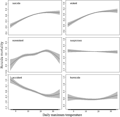
Finally, analysis by method of suicide showed that when the temperature increased the suicide rate increased only for violent methods. For the other methods, the pattern of the relation remained unclear, probably due to the few suicide deaths on the individual days (Fig. 8).

Fig. 8.

The GAM-estimated effect of maximum temperature on suicide mortality for different methods. This is an example of the Tohoku region, where the suicide mortality was highest. The continuous lines are the function estimates, and the shaded areas delimit the 95% confidence interval for the function. The numbers on each y-axis are the effective degrees of freedom of the term being plotted. Smoothing parameters are estimated by UBRE/AIC

Discussion

Alternative designs

To identify the relation between suicide mortality and maximum temperature and to show whether the choice of the design affected the results, the time-series with the Poisson generalized linear regression model (GLM) [34], and the conditional fixed-effect Poisson [38] regression model were used.

In the GLM to control for unobserved time-varying covariates, we introduced linear and cubic trends to control for any overall trend, sinusoidal terms to control for seasonality, and indicator variables for weekdays and public holidays to control for weekly variations. The covariates considered were maximum temperatures, relative humidity, atmospheric pressure, and sunshine duration.

The variables included in the model were chosen individually on the basis of their respective levels of significance, and jointly on the basis of those that minimized the AIC criterion [36]. Once the best-fit model was selected with the support of Pearson residuals, we then tested for overdispersion using the dispersion parameter (φ), and for residual autocorrelation using the simple (ACF) and partial autocorrelation function (PACF) plots.

A conditional fixed-effect model is formed by conditioning out the fixed effects from the estimation. This allows a much more efficient estimator at the cost of placing constraints on inference in the form of the conditioning imposed on the likelihood. The strength of the analysis is that it was possible to control for season and year confounders by means of design. This is similar to case-crossover design [39]. Other confounding factors were included in the model in the same manner as for the GLM model.

All models yielded very similar results. The pattern of the relation for all regions was similar to the one derived from using the GAM analysis (results are not shown), although the confidence intervals were wider.

Comparing results with other studies

After controlling for the seasonal pattern in suicide mortality we found a short-term effect of daily maximum temperature on suicide, which was consistent with the study conducted by Page and colleagues [15]. Page et al. found the highest monthly number of deaths from suicide taking place in January. In contrast, we obtained the first (and highest) year peak in suicide in April and the second in October. The winter shift is probably due to the fact that in England the fiscal year starts in January, while in Japan the year begins in April. However, the elevated suicide mortality in spring in Japan can probably be explained almost entirely by economic, social, and demographic trends or by the historical background of Japanese suicide rather than by the physical environmental factors.

There is a belief that melatonin (opposite to vitamin D) may play a significant role in suicide deaths [40], as this hormone’s production is stimulated by the absence of light. With regard to this matter, the hours of daylight may be a better predictive factor than the sunshine duration, although the hours of daylight might confound the relation between temperature and suicide on a seasonal timescale (Fig. 7).

As for the day of week, we also found that the largest number of suicide deaths occurred on Mondays, although this might have been confounded by the actual time of reporting a suicide death.

Finally, our results confirmed the association of violent suicide methods with high temperatures; that is, when temperature increased the suicide mortality increased mostly for violent methods. The pattern of the relation for other methods remained unclear.

Various mechanisms might underlie the effect of high temperatures on suicide, which can be based on the sociological, biological, or psychological assumptions of suicidal behavior [15]. Sociological and biological mechanisms can probably be used to explain long-term rhythms in suicide, such as annual or seasonal rhythms [41], while a psychological mechanism is the most promising one to link suicide with high temperatures on a short-term scale [15].

Conclusion

Suicide is a serious public health problem and suicide prevention is a major public health challenge and one of the key elements of current mental health policy. Recognizing that high temperatures confer a great risk for suicidal behavior is an important step toward continued efforts to improve the scientific basis of suicide prevention.

The present study has shown that an increase in temperature has a short-term effect on suicide mortality in Japan. However, further investigations, possibly including spatial analysis, should be considered.

References

- 1.Araki S, Murata K. Suicide, religion, and socioeconomic conditions. Tohoku J Exp Med. 1986;149(2):205–211. doi: 10.1620/tjem.149.205. [DOI] [PubMed] [Google Scholar]
- 2.Akechi T, Iwasaki M, Uchitomi Y, Tsugane S, JPHC Study Group Alcohol consumption and suicide among middle-aged men in Japan. Br J Psychiatry. 2006;188:231–236. doi: 10.1192/bjp.188.3.231. [DOI] [PubMed] [Google Scholar]
- 3.Salih MA. Suicide pact in a setting of Folie a Deux. Br J Psychiatry. 1981;139:62–67. doi: 10.1192/bjp.139.1.62. [DOI] [PubMed] [Google Scholar]
- 4.Thompson S. The internet and its potential influence on suicide. Psychiatr Bull R Coll Psychiatr. 1999;23:449–451. doi: 10.1192/pb.23.8.449. [DOI] [Google Scholar]
- 5.Becker K, Mayer M, Nagenborg M, El-Faddagh M, Schmidt MH. Parasuicide online: can suicide websites trigger suicidal behaviour in predisposed adolescents? Nord J Psychiatry. 2004;58:111–114. doi: 10.1080/08039480410005602. [DOI] [PubMed] [Google Scholar]
- 6.Rajagopal S. Suicide pacts and the internet. Br Med J. 2004;329(7478):1298–1299. doi: 10.1136/bmj.329.7478.1298. [DOI] [PMC free article] [PubMed] [Google Scholar]
- 7.Rockett IR, Smith GS. Covert suicide among elderly Japanese females: questioning unintentional drownings. Soc Sci Med. 1993;36(11):1467–1472. doi: 10.1016/0277-9536(93)90388-K. [DOI] [PubMed] [Google Scholar]
- 8.Deisenhammer EA. Weather and suicide: the present state of knowledge on the association of meteorological factors with suicidal behaviour. Acta Psychiatr Scand. 2003;108:402. doi: 10.1046/j.0001-690X.2003.00209.x. [DOI] [PubMed] [Google Scholar]
- 9.Lambert G, Reid C, Kaye D, Jennings G, Esler M. Increased suicide rate in the middle-aged and its association with hours of sunlight. Am J Psychiatry. 2003;160:793–795. doi: 10.1176/appi.ajp.160.4.793. [DOI] [PubMed] [Google Scholar]
- 10.Parker G, Walter S. Seasonal variation in depressive disorders and suicidal deaths in New South Wales. Br J Psychiatry. 1982;140:626–632. doi: 10.1192/bjp.140.6.626. [DOI] [PubMed] [Google Scholar]
- 11.Partonen T, Haukka J, Pirkola S, Isometsä E, Lönnqvist J. Time patterns and seasonal mismatch in suicide. Acta Psychiatr Scand. 2004;109:110–115. doi: 10.1046/j.0001-690X.2003.00226.x. [DOI] [PubMed] [Google Scholar]
- 12.Preti A. The influence of seasonal change on suicidal behaviour in Italy. J Affect Disord. 1997;44:123–130. doi: 10.1016/S0165-0327(97)00035-9. [DOI] [PubMed] [Google Scholar]
- 13.Preti A, Miotto P. Influence of method on seasonal distribution of attempted suicides in Italy. Neuropsychobiology. 2000;41:62–72. doi: 10.1159/000026635. [DOI] [PubMed] [Google Scholar]
- 14.Sato T. Seasonality of suicides (letter) Br J Psychiatry. 2001;178:183. doi: 10.1192/bjp.178.2.183-a. [DOI] [PubMed] [Google Scholar]
- 15.Page L, Hajat S, Kovats RS. Relationship between daily suicide counts and temperature in England and Wales. Br J Psychiatry. 2007;191:106–112. doi: 10.1192/bjp.bp.106.031948. [DOI] [PubMed] [Google Scholar]
- 16.Nicholls N, Butler CD, Hanigan I. Inter-annual rainfall variations and suicide in New South Wales, Australia, 1964–2001. Int J Biometeorol. 2006;50:139–143. doi: 10.1007/s00484-005-0002-y. [DOI] [PubMed] [Google Scholar]
- 17.Salib E. Elderly suicide and weather conditions: is there a link? Int J Geriatr Psychiatry. 1997;12:937–941. doi: 10.1002/(SICI)1099-1166(199709)12:9<937::AID-GPS667>3.0.CO;2-O. [DOI] [PubMed] [Google Scholar]
- 18.Chiu LPW. Do weather, day of the week, and address affect the rate of attempted suicide in Hong Kong? Soc Psychiatry Psychiatr Epidemiol. 1988;23:229–235. doi: 10.1007/BF01787822. [DOI] [PubMed] [Google Scholar]
- 19.Digon E, Block HB. Suicides and climatology. Arch Environ Health. 1966;12:276–289. doi: 10.1080/00039896.1966.10664374. [DOI] [PubMed] [Google Scholar]
- 20.Dixon KW, Shulman MD. A statistical investigation into the relationship between meteorological parameters and suicide. Int J Biometeorol. 1983;27:93–105. doi: 10.1007/BF02185738. [DOI] [PubMed] [Google Scholar]
- 21.Pokorny AD, Davis F, Harberson W. Suicide, suicide attempts, and weather. Am J Psychiatry. 1963;120:377–381. doi: 10.1176/ajp.120.4.377. [DOI] [PubMed] [Google Scholar]
- 22.Pokorny AD. Suicide and weather. Arch Environ Health. 1966;13:225–256. doi: 10.1080/00039896.1966.10664543. [DOI] [PubMed] [Google Scholar]
- 23.Patz JA, Campbell-Lendrum D, Hollowway T, Foley JA. Impact of regional climate change on human health. Nature. 2005;438:310–317. doi: 10.1038/nature04188. [DOI] [PubMed] [Google Scholar]
- 24.Speckman P. Kernel smoothing in partial linear models. J R Stat Soc Series B Stat Methodol. 1988;50:413–436. [Google Scholar]
- 25.Hastie TJ, Tibshirani RJ. Generalized additive models. London: Chapman & Hall; 1990. [Google Scholar]
- 26.Green PJ, Silverman BW. Nonparametric regression and generalized linear models: a roughness penalty approach. London: Chapman & Hall; 1994. [Google Scholar]
- 27.Marx BD, Eilers PHC. Direct generalized additive modeling with penalized likelihood. Comput Stat Data Anal. 1998;28:193–209. doi: 10.1016/S0167-9473(98)00033-4. [DOI] [Google Scholar]
- 28.Dominici F, McDermott A, Hastie T. Improved semi-parametric time series models of air pollution and mortality. J Am Stat Assoc. 2004;468:938–948. doi: 10.1198/016214504000000656. [DOI] [Google Scholar]
- 29.Peng RD, Dominici F, Louis TA. Model choice in time series studies of air pollution and mortality. Berkeley: BEP; 2005 (Paper 55).
- 30.Schwartz J. Generalized additive models in epidemiology. In: International Biometric Society, Invited Papers. 17th International Biometric Conference. Hamilton, ON: International Biometric Society; 1994. p. 55–80.
- 31.Craven P, Wahba G. Smoothing noisy data with spline functions. Appl Numer Math. 1979;31:377–403. [Google Scholar]
- 32.Ihaka R, Gentlemen R. R: a language for data analysis and graphics. J Comput Graph Stat. 1996;5:299–314. http://www.R-project.org.
- 33.Crawley MJ. The R book. New York: Wiley; 2007. [Google Scholar]
- 34.McCullagh P, Nelder J. Generalized linear models. 2. London: Chapman & Hall; 1989. [Google Scholar]
- 35.NIST/SEMATECH e-Handbook of statistical methods. 2008. http://www.itl.nist.gov/div898/handbook/.
- 36.Akaike H. Information theory and an extension of the maximum likelihood principle. In: Petrov BN, Csáki F, editors. 2nd international symposium on information theory. Budapest: Akademia Kiao; 1973. pp. 267–281. [Google Scholar]
- 37.Armstrong B. Models for the relationship between ambient temperature and daily mortality. Epidemiology. 2006;17(6):624–631. doi: 10.1097/01.ede.0000239732.50999.8f. [DOI] [PubMed] [Google Scholar]
- 38.Hausman JA, Hall BH, Griliches Z. Econometric models for count data with an application to the patents-R&D relationship. Econometrica. 1984;52(4):909–938. doi: 10.2307/1911191. [DOI] [Google Scholar]
- 39.Maclure M. The case-crossover design: a method for studying transient effects on the risk of acute events. Am J Epidemiol. 1991;133:144–153. doi: 10.1093/oxfordjournals.aje.a115853. [DOI] [PubMed] [Google Scholar]
- 40.Petridou E, Paradopoulos FC, Frangakis CE, Skalkidou A, Trichopoulos D. A role of sunshine in the triggering of suicide. Epidemiology. 2002;13:106–109. doi: 10.1097/00001648-200201000-00017. [DOI] [PubMed] [Google Scholar]
- 41.Salib E, Cortina-Borja M. Effect of month of birth on the risk of suicide. Br J Psychiatry. 2006;188(5):416–422. doi: 10.1192/bjp.bp.105.009118. [DOI] [PubMed] [Google Scholar]