

Abstract
Existing models of electrical activity in myocardial tissue are unable to easily capture the effects of ephaptic coupling. Homogenized models do not account for cellular geometry, while detailed spatial models are too complicated to simulate in three dimensions. Here we propose a unique model that accurately captures the geometric effects while being computationally efficient. We use this model to provide an initial study of the effects of changes in extracellular geometry, gap junctional coupling, and sodium ion channel distribution on propagation velocity in a single 1D strand of cells. In agreement with previous studies, we find that ephaptic coupling increases propagation velocity at low gap junctional conductivity while it decreases propagation at higher conductivities. We also find that conduction velocity is relatively insensitive to gap junctional coupling when sodium ion channels are located entirely on the cell ends and cleft space is small. The numerical efficiency of this model, verified by comparison with more detailed simulations, allows a thorough study in parameter variation and shows that cellular structure and geometry has a nontrivial impact on propagation velocity. This model can be relatively easily extended to higher dimensions while maintaining numerical efficiency and incorporating ephaptic effects through modeling of complex, irregular cellular geometry.
Keywords: cardiac electrophysiology, extracellular conductivity, microdomain effects
While gap junctional coupling is usually considered to be the primary mechanism for action potential propagation, there is evidence that other mechanisms are important. In particular, only a moderate reduction of cardiac propagation velocity was found in murine hearts with inactivated Connexin43 (Cx43) gene (1). In mice with heterozygous Cx43 ± down-regulation, either a 23–44% decrease in propagation velocity (2–4) or no discernible decrease in propagation velocity (5–8) was found. In Cx43 - /- mice with no expression of the protein, propagation was still found, although discontinuous and at much slower speeds (7). These experimental findings are in conflict with the classical understanding of how gap junctions determine propagation velocity.
One possible explanation for these intriguing observations is that ephaptic (i.e., field effect) coupling may be significant (1, 9–12). However, the study of ephaptic effects is made difficult by the fact that these effects are most important in microdomains such as junctional clefts.
Existing homogenized models, while computationally accessible, are not able to deal with the effects of microdomains and hence do not capture the effects of ephaptic coupling (13, 14). On the other hand, detailed spatial models have shown that geometry plays an important role in the conduction velocity but are too expensive to implement for a full 3D tissue (11, 12, 15–19).
Here we present a model that captures the effects of the intricate cellular geometry with simplifications that will allow the model to be extended more readily to three dimensions while maintaining computational efficiency. With this model we expect to be able to study the effects of changes in geometry (for example, due to hydration or dehydration) and pathology (such as ischemia) on propagation velocity.
In this paper, we present the model and show results of simulation for an idealized 1D strand of cardiac cells. We find that ephaptic coupling increases propagation velocity at low gap junctional conductivity while it decreases propagation at higher conductivities. We also find that conduction velocity is relatively insensitive to gap junctional coupling when ionic channels are located entirely in the junctional clefts and junctional space is small. The consistency of these results with previous findings (11) and a comparative study with a more detailed model presented in Discussion validate the assumptions made in this model.
The Model
The complicated structure of cardiac myocytes cells can be described as intercalated, irregular bricks. These long cells are surrounded by a thin layer of extracellular space, of which the junctional cleft is particularly narrow and tortuous. The two domains, the intracellular and extracellular spaces, are separated by cell membranes. We expect that the complicated geometry can cause the electrical interactions to also be highly irregular.
The classical derivation of the equations for action potential propagation makes use of cable theory, in which the extracellular resistance is assumed to be isopotentially zero and the intracellular space conductivity is taken to be proportional to the cross-sectional area of the cell (11, 20). While this is the appropriate approximation for axons in a bath, it may not be so for cardiac cells. In fact, the bidomain model allows for resistance in both the intracellular and extracellular spaces.
Ephaptic coupling occurs because the junctional space resistivity is high and therefore is not isopotential with the rest of extracellular domain. This is the result of the small cross-sectional area in the narrow gaps between the ends of cells. With this realization, it seems apparent that it is the resistivity of the extracellular space that is the most important determinant of propagation velocity, not the resistivity of intracellular space. Thus, in the model here, we make the assumption that the intracellular space of each cell is isopotential and the extracellular potential is spatially varying. Quantitatively, the resistance in the intracellular space is subdominant to that of the extracellular space. The intracellular conductivity of 6.7 mS/cm (21) with cell radius 0.001317 cm (cell diameter is approximately 1/6 of the cell length 0.0158 cm) (13) gives rise to an intracellular longitudinal conductance of 6.7(π0.0013172)/0.0158 ≈ 2.3 × 10⁻³ mS. The extracellular conductivity of 20 mS/cm with extracellular width 1.33 × 10⁻⁵ cm (see Table 1) gives rise to an approximate extracellular longitudinal conductance of 20(2π)(0.001317)(1.33 × 10⁻⁵)/0.0158 ≈ 1.39 × 10⁻⁴ mS. Similar calculations can be done for the transverse conductances. Because the intracellular conductance is at least an order of magnitude larger than that of the extracellular space, we make the simplifying assumption that the intracellular space is represented by a single potential, whereas the potential in the extracellular space requires detailed spatial resolution. The validity of this assumption is further corroborated by a comparison with a more detailed model (see Discussion section), in which the intracellular potential is allowed to vary in space. This assumption is also consistent with the results of ref. 16, in which a detailed 3D model shows isopotential cellular interiors with spatially varying extracellular potentials. Additionally, given the narrow gaps between cells, the extracellular potential is assumed to be uniform across the shortest distance between cells. This enables us to view the extracellular space as a 2D surface rather than a 3D volume. The width of the extracellular space is factored into the computation of the conductivity of the 2D surface at any given position.
Table 1.
Parameter values


The setup is as follows: The jth cell occupies the space Ωj. The extracellular space is the complement of intracellular space; however, because this is generally quite thin, we view extracellular space as the 2D surface of 3D cells, hence the extracellular space is Ωe = ∪j∂Ωj. Notice that the junctional clefts are part of extracellular space. For each point x in the extracellular space there are κ(x) adjoining cells specified by the index set E(x). For x on the boundary of the tissue, κ(x) = 1, and otherwise κ(x) = 2 (with the exception of points at corners, which will not matter in what follows). Similarly, each cell has neighbors to which it is coupled by gap junctions, denoted by the indices Ij. We denote the gap junctional coupling strength between cell j and its neighbors by gjk(x) for k∈Ij and gjk can be nonzero only for x such that cells j and k are adjoining (i.e., x∈∂Ωj∩∂Ωk). The membrane capacitance is denoted by Cm, extracellular conductivity by Ce, extracellular width by W(x), ionic currents by  , intracellular potential by
  , and extracellular potential ϕe. See Figs. 1 and 2 for the idealized geometrical and discretized electrical notations.
Fig. 1.

Notation for a cylindrical strand of cells.
Fig. 2.

Discretized electrical circuit diagram for cells.
Current conservation in the extracellular space is
 |
[1] |
and current conservation in the intracellular space is
 |
[2] |
where χj = ∫∂Ωjdx is the total surface area of the jth cell. We rearrange these to put them into a somewhat familiar form,
 |
[3] |
 |
[4] |
Methods
This system of differential equations can be written in the form
 |
[5] |
where A and L are linear operators, L being a Laplacian-like operator. For numerical simulations, A and L are spatially discretized (see Fig. 2) via a standard cell-centered finite difference scheme, with resultant operators  and
and  . Because these equations resemble a parabolic system, we use the Crank–Nicholson scheme, where Φn = Φ(t = tn), for temporal discretization
 |
[6] |
providing a method to update the potentials of the system.
For an initial study of the effects of the geometry of extracellular space on conduction, we consider a single strand of cylindrically symmetric cardiac cells. The entire strand is surrounded by a layer of extracellular space, and neighboring cells are separated by narrow junctional clefts. Cells are also connected end-to-end by uniformly distributed gap junctions (see Fig. 1). Ionic currents are given by the simplified Beeler–Reuter equations,
| [7] |
where iK, iNa, and il represent the currents from the potassium ions, sodium ions, and leakage component; details are given in Appendix. In Eq. 7, θ(x) represents the distribution of sodium ion channels at position x, with θ(x) = θj if x is in the junctional space and θ(x) = θm elsewhere on the membrane. We include this parameter due to experimental evidence of increased density of sodium channels on cell ends (10, 11, 22, 23). The total number of sodium ion channels is held constant, so that
 |
[8] |
where Aj is the surface area of one end of a single cell, χj = AT, for all j, is the total surface area of a single cell, and Am = AT - 2Aj. Thus, at the nominal values of  , the sodium channels are evenly distributed on the surface of the cell.
Voltage is applied on the ends of the strand, injecting current into the strand until an end cell is spiked into an action potential. The speed of propagation and behavior of the change in potentials is studied as the action potential travels along the length of the strand. Three parameters—the effective conductivity in the junctional cleft Cefft = W(x)Ce, the gap junctional conductivity gjk, and the distribution of sodium ion channels θ(x)—are varied in this study.
For the data reported in this paper, we constructed a strand of 20 myocytes. Each cell is 0.00263 cm in diameter and 0.0158 cm in length (13) with a spatial discretization of dx = 0.000263 cm, giving rise to 10 grid points along the diameter of the cell and 60 grid points along the longitudinal edge of each cell. With the given simplifications of this model and taking advantage of cylindrical symmetry, this strand of cells has 1,325 unknowns. Extracellular volume was initally assumed to be approximately 10% of the total volume (14). Because only 20% of this extracellular space is electrically conducting (24), we reduce the volume accordingly (removing capillaries, plasma, etc.) and take an approximate value of 2% of the total volume for the extracellular space. The intracellular potentials are initiated at -70 mV, whereas the extracellular space is initially at 0 mV. No current is allowed to pass through the external boundary of the extracellular space except at the ends of the strand, which are held at +30 mV and -30 mV until the average transmembrane potential of the end cell exceeds -10 mV. After the end cell is spiked, no current is allowed to pass through the entire external boundary of the extracellular space. This process mimics experimental procedures that inject current into myocardial tissue to induce an action potential. Sodium ion channel density not on the ends of the cell θm, gap junctional conductivity gjk, and effective conductivity in the junctional cleft Cefft have nominal values of  ,
,  , and
, and  , respectively. A summary of these values and other parameters is given in the Table 1.
Conduction speed is calculated by measuring the time between when the average transmembrane potential of the first cell reaches a specified threshold value and the 17th cell reaches the same threshold. The distance between those two points is fixed by the length of the cells and the width of the junctional clefts.
Results
With the parameters given above, we began by looking at the nonephaptic case, in which none of the sodium ion channels are located on the ends of cells (θj = 0, θm = AT/Am). In this regime, the effective conductivity in the junctional cleft simply affects the propagation of the action potential through diffusion into the longitudinal extracellular space and, because the cleft is so narrow compared to the rest of the extracellular space, this has an insignificant effect on the conduction speed (this can be seen in the lower left plot of Fig. 5). Fig. 3 shows the conduction speed for varying gap junctional conductivities, with conduction failure occurring at small values. This is in agreement with the results found in ref. 20.
Fig. 5.

Propagation velocities as the gap junction conductivity changed between 0% and 100% of its nominal value. (Top) Trends are shown as the junctional cleft width varies from 0% to 100% of its nominal value, for differing ionic channel distributions. (Bottom) Trends are shown as the junctional cleft width varies from 0% to 100% of its nominal value, for differing gap junctional coupling.
Fig. 3.

Conduction speeds in the nonephaptic case ( ), with varying gap junctional conductivities. Extracellular effective junctional conductivities have little effect on the curve at these scales.
In general, we found that propagation can be characterized as in one of two cases: one in which the extracellular junctional cleft potentials lag behind the action potential and one in which the cleft potentials lead the action potential. Fig. 4 shows time series plots of the transmembrane potentials (full movies can be found in Movies S1 and S2). To plot these potentials, we number the extracellular space sequentially by running along the longitudinal edge of the cell strand, dipping halfway down and back out of the junctional clefts at corners of cells to calculate the transmembrane potential arising from cells on each side of the junctional cleft. Note that in the junctional space, there is a single, spatially varying extracellular potential, but that at each point of the junctional cleft, there are two different transmembrane potentials due to differing intracellular potentials of the neighboring cells. Fig. 4A shows the transmembrane potentials in the junctional-lagging case. The distinct dip in potential in the clefts is shown in gray in each plot, as the action potential travels from right to left and the junctional cleft potentials increase primarily by diffusion from the rest of the extracellular space. Fig. 4B shows the junctional-leading case, where the potentials in the cleft at the propagation front are higher than those of the extracellular space around the rest of the cell. We remark here that while junctional-lagging and junctional-leading effects can be elicited in different ways to varying degrees, for these simulations junctional-lagging clefts were created by removing all sodium ion channels in the clefts and reducing the conductivity in the extracellular clefts to 15% of the nominal value. Junctional-leading, on the other hand, was produced by distributing all the channels to the ends of cells and allowing the conductivity in the clefts to remain at its nominal value. Gap junctional conductivity in both these cases was kept at its nominal value.
Fig. 4.

Time series plots of transmembrane potentials in the case of (A) lagging clefts and (B) leading clefts for an action potential moving from right to left.
For a complete study of the parameter variation, we change the conductivity of the gap junctions, the distribution of the sodium ion channels, and the width of the junctional cleft and find the resulting propagation speeds. In Fig. 5, we show conduction velocities for gap junctional conductivities gjk that range from 0% to 100% of the nominal conductivity values. The distribution of nonjunctional sodium ion channels θm ranges from 0 to AT/Am, which is from 0% to 108.3% of its nominal value of 1. The width of the junctional cleft varied in such a way that the effective conductivity Cefft changed between 0% and 100% of its nominal value. At low gap junctional conductivities, ephaptic effects generally increase the conduction velocity, whereas at high gap junctional conductivities, the ephaptic effects are slightly deleterious. This is evident in the reversal of trends shown from left to right in the top panel of Fig. 5. Additionally, for small junctional clefts widths, as the ionic channels are distributed more heavily to the ends of the cells, the gap junctional conductivity plays a smaller and smaller role in determining the conduction velocity. The bottom panel of Fig. 5 shows the curves of conduction speeds appearing to collapse together at small cleft widths as the distribution of channels is increasingly placed on the ends of cells.
Discussion
We have presented a unique approach to modeling the electrical coupling of myocardial cells by assuming an isopotential cellular interior, along with a 2D extracellular space. This model, given by Eqs. 3 and 4, can be simulated more efficiently than a full 3D model, yet is able to capture the effects of the details of cellular geometry. Our initial study of a 1D strand of cells shows that the fraction of extracellular space [in changing W(x)Ce in the extracellular space at the ends of the cells] affects the propagation speed greatly, in agreement with ref. 19. We also find that with large gap junctional conductivity, the decreased conductivity in the junctional cleft leads to an increase in propagation speed, agreeing with previous numerical studies (11, 18). At low gap junctional conductivities, the ephaptic coupling increases action potential propagation speed and can even prevent conduction failure in the case of no gap junctional coupling, similar to findings by (11, 12).
The assumption of an isopotential intracellular space, based on relative conductances, can be further studied by a numerical comparison between our model and one in which the intracellular space has been discretized in the longitudinal direction. Fig. 6 shows the results of this comparison. The potential gradient at the moving front of the action potential in the intracellular space is subdominant to that of the extracellular space. When all parameters are taken at nominal values, the error in propagation velocity caused by smoothing out the intracellular potential is approximately 0.4%. Any reduction in the coupling from nominal value results in decreasing the steepness of intracellular potential gradients, amplifying the dominance of the extracellular potential gradient.
Fig. 6.

The potentials of the detailed and simplified models are closely matched at nominal values. The intracellular potential gradients at the front of the action potential are subdominant to those of the extracellular space. (Inset) The intracellular gradient seen in the detailed model is flattened in the simplified model.
For large gap junctional conductivity, ephaptic effects are mostly deleterious. As the conductivity in the clefts decrease, the cell ends depolarize quickly and do not aid in the positive feedback loop of the ionic current that is necessary to enhance the propagation speed. Additionally, reduced conductivity in the clefts slows the diffusion into the rest of the extracellular space. These two effects lower the propagation speed from that of the nominal values.
As the gap junctional conductivity decreases, the baseline (shown in gray in the top panel of Fig. 5), in which none of the ionic channels are on the ends of the cell, decreases steadily. For small gap junctional coupling, cell-to-cell communication depends heavily on the cleft space. Small cleft width and sodium channels that favor the ends of the cells will greatly enhance propagation speeds through ephaptic effects (see Movies S3 and S4).
At small cleft conductivities and with ionic channel distributions that favor the ends of the cells, the coupling of the gap junctions has a less dramatic effect on the propagation velocity. Localization of ionic channels on the ends of cells has been shown in several studies (10, 11, 22, 23), and in conjunction with our findings, may provide an explanation for the slight reduction in conduction speeds with the down-regulation of Cx43 found in experiments (1).
The parameters taken in this study are values extracted from experimental data. However, there is a large variation in the literature as to the range of these values. Changing the parameters that we use here will have a quantitative, but not qualitative, difference in the results. The trends established here by parameter variation make it clear that the complex cellular structure has a nontrivial and significant impact on the propagation velocity of an action potential. Similarly, the qualitative nature of these trends is not affected significantly by the details of the ionic currents, such as L-type calcium or other fast inward sodium channel descriptions.
A fundamental difference between our model and that of ref. 11 is that we take cells to be isopotential, while in ref. 11 extracellular space is taken to be isopotential. This feature of our model, which we have shown to be quantitatively valid, not only makes it computationally more tractable for higher dimensional tissue while still providing accurate results, but also allows us to incorporate complex, irregular geometry of cells. By allowing variations in the width of the extracellular microdomain (this cannot be done if the extracellular space is taken to be isopotential, which is a common assumption), we will additionally be able to investigate possible side-to-side, nonjunctional ephaptic effects. We have shown in this study that ephaptic effects have the potential to greatly modify propagation speed. Such modeling is critical for realistic simulation of myocardial tissue.
In the future, we will study the effect of parameter variation in higher dimensional tissue with other additions, such as additional ionic currents. With this model, we will be able to study different geometries of cells and explore the dependence of ephaptic effects on sodium ion channel distribution and extracellular width. The simplifications we have presented in this paper improve upon existing microscale models, which can be used in a multiscale model to fully simulate myocardial tissue. Furthermore, the results of our 1D study suggest that extracellular currents cannot be neglected, and the approach described here could have a significant impact on our understanding of cardiac excitation propagation.
Appendix
Ionic currents for the simplified Beeler–Reuter equations:
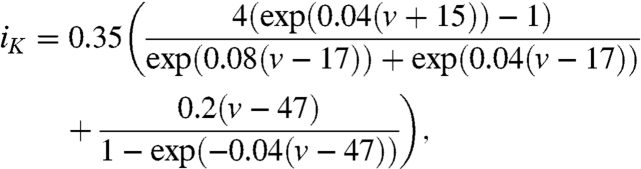 |
[9] |
 |
[10] |
 |
[11] |
| [12] |
where  is the transmembrane potential. Here Veq represents the equilibrium potential of -70 mV.
Supplementary Material
Acknowledgments.
This research is supported in part by National Science Foundation (NSF) Grant DMS-0602219 (J.L.), and in part by NSF Grant DMS-0718036 (J.P.K.).
Footnotes
The authors declare no conflict of interest.
This article is a PNAS Direct Submission.
This article contains supporting information online at www.pnas.org/lookup/suppl/doi:10.1073/pnas.1010154107/-/DCSupplemental.
References
- 1.Yao J-A, Gutstein DE, Liu F, Fishman GI, Wit AL. Cell coupling between ventricular myocyte pairs from connexin43-deficient murine hearts. Circ Res. 2003;93:736–743. doi: 10.1161/01.RES.0000095977.66660.86. [DOI] [PubMed] [Google Scholar]
- 2.Guerrero P, et al. Slow ventricular conduction in mice heterozygous for a Connexin43 null mutation. J Clin Invest. 1997;99:1991–1998. doi: 10.1172/JCI119367. [DOI] [PMC free article] [PubMed] [Google Scholar]
- 3.Thomas SA, et al. Disparate effects of deficient expression of connexin43 on atrial and ventricular conduction: Evidence for chamber-specific molecular determinants of conduction. Circulation. 1998;97:686–691. doi: 10.1161/01.cir.97.7.686. [DOI] [PubMed] [Google Scholar]
- 4.Eloff BC, et al. High resolution optical mapping reveals conduction slowing in connexin43 deficient mice. Cardiovasc Res. 2001;51:681–690. doi: 10.1016/s0008-6363(01)00341-8. [DOI] [PubMed] [Google Scholar]
- 5.Morley GE, et al. Characterization of conduction in the ventricles of normal and heterozygous cx43 knockout mice using optical mapping. J Cardiovasc Electr. 1999;10:1361–1375. doi: 10.1111/j.1540-8167.1999.tb00192.x. [DOI] [PubMed] [Google Scholar]
- 6.Vaidya D, et al. Null mutation of connexin43 causes slow propagation of ventricular activation in the late stages of mouse embryonic development. Circ Res. 2001;88:1196–1202. doi: 10.1161/hh1101.091107. [DOI] [PubMed] [Google Scholar]
- 7.Beauchamp P, et al. Electrical propagation in synthetic ventricular myocyte strands from germline connexin43 knockout mice. Circ Res. 2004;95:170–178. doi: 10.1161/01.RES.0000134923.05174.2f. [DOI] [PubMed] [Google Scholar]
- 8.Thomas SP, et al. Impulse propagation in synthetic strands of neonatal cardiac myocytes with genetically reduced levels of connexin43. Circ Res. 2003;92:1209–1216. doi: 10.1161/01.RES.0000074916.41221.EA. [DOI] [PMC free article] [PubMed] [Google Scholar]
- 9.Copene ED, Keener JP. Ephaptic coupling of cardiac cells through the junctional electric potential. J Math Biol. 2008;57:265–284. doi: 10.1007/s00285-008-0157-3. [DOI] [PubMed] [Google Scholar]
- 10.Sperelakis N, McConnell K. Electric field interactions between closely abutting excitable cells. IEEE Eng Med Biol Mag. 2002;21:77–89. doi: 10.1109/51.993199. [DOI] [PubMed] [Google Scholar]
- 11.Kucera JP, Rohr S, Rudy Y. Localization of sodium channels in intercalated discs modulates cardiac conduction. Circ Res. 2002;91:1176–1182. doi: 10.1161/01.res.0000046237.54156.0a. [DOI] [PMC free article] [PubMed] [Google Scholar]
- 12.Mori Y, Fishman GI, Peskin CS. Ephaptic conduction in a cardiac strand model with 3d electrodiffusion. Proc Natl Acad Sci USA. 2008;105:6463–6468. doi: 10.1073/pnas.0801089105. [DOI] [PMC free article] [PubMed] [Google Scholar]
- 13.Hand PE, Griffith BE, Peskin CS. Deriving macroscopic myocardial conductivities by homogenization of microscopic models. B Math Biol. 2009;71:1707–1726. doi: 10.1007/s11538-009-9421-y. [DOI] [PubMed] [Google Scholar]
- 14.Neu J, Krassowska W. Homogenization of syncytial tissues. Crit Rev Biomed Eng. 1993;21:137–199. [PubMed] [Google Scholar]
- 15.Stinstra JG, Hopenfeld B, MacLeod RS. On the passive cardiac conductivity. Ann Biomed Eng. 2005;33:1743–1751. doi: 10.1007/s10439-005-7257-7. [DOI] [PubMed] [Google Scholar]
- 16.Stinstra JG, MacLeod RS, Henriquez CS, A comparison between a 3D microscropic model of anisotropic conduction in cardiac tissue and the bidomain model. in press. [Google Scholar]
- 17.Mori Y, Jerome JW, Peskin CS. A three-dimensional model of cellular electrical activity. Bulletin of the Institute of Mathematics, Academia Sinica. 2007;2:367–390. [Google Scholar]
- 18.Roberts SF, Stinstra JG, Henriquez CS. Effect of nonuniform interstitial space properties on impulse propagation: A discrete multidomain model. Biophys J. 2008;95:3724–3737. doi: 10.1529/biophysj.108.137349. [DOI] [PMC free article] [PubMed] [Google Scholar]
- 19.Stinstra JG, Roberts SF, Pormann JB, MacLeod RS, Henriquez CS. A model of 3D propagation in discrete cardiac tissue. Comput Cardiol. 2006;33:41–44. [PMC free article] [PubMed] [Google Scholar]
- 20.Hand PE, Griffith BE, An adaptive multiscale model for simulating cardiac conduction. doi: 10.1073/pnas.1008443107. in press. [DOI] [PMC free article] [PubMed] [Google Scholar]
- 21.Shaw RM, Rudy Y. Roles of the sodium and L-type calcium currents during reduced excitability and decreased gap junction coupling. Circ Res. 1997;81:727–741. doi: 10.1161/01.res.81.5.727. [DOI] [PubMed] [Google Scholar]
- 22.Maier SK, et al. An unexpected role for brain-type sodium channels in coupling of cell surface depolarization to contraction in the heart. Proc Natl Acad Sci USA. 2002;99:4073–4078. doi: 10.1073/pnas.261705699. [DOI] [PMC free article] [PubMed] [Google Scholar]
- 23.Cohen SA. Immunocytochemical localization of rH1 sodium channel in adult rat heart atria and ventricle. Presence in terminal intercalated disks. Circulation. 1996;94:3083–3086. doi: 10.1161/01.cir.94.12.3083. [DOI] [PubMed] [Google Scholar]
- 24.Frank JS, Langer GA. The myocardial interstitium: Its structure and its role in ionic exchange. J Cell Biol. 1974;60:586–601. doi: 10.1083/jcb.60.3.586. [DOI] [PMC free article] [PubMed] [Google Scholar]
- 25.Weidmann S. Electrical constants of trabecular muscle from mammalian heart. J Physiol. 1970;210:1041–1054. doi: 10.1113/jphysiol.1970.sp009256. [DOI] [PMC free article] [PubMed] [Google Scholar]
Associated Data
This section collects any data citations, data availability statements, or supplementary materials included in this article.