Matching models to data: a receptor pharmacologist's guide

Abstract

In this review we discuss a number of topics related to fitting mechanistic mathematical models to experimental data. These can be divided broadly into issues to consider before beginning an experiment or fitting a model and the advantages of direct fitting of a model over other methods of analysis (e.g. null methods).

We have sought to address some commonplace issues of receptor pharmacology with some real-life examples: How should dilutions be distributed along a concentration–response curve? How do problems with dilutions manifest in assay results? What assumptions are made when certain analysis models are applied? What is global data fitting and how does it work? How can it be applied to improve data analysis? How can models such as one-site and two-site fits be compared? What is the principal behind statistical comparison of data fits?

It is our hope that after reading this review you will have a greater appreciation of assay planning and subsequent data analysis and interpretation which will improve the quality of the data that you generate.

Introduction

The aim of a pharmacological experiment can be summarized in one of two ways: identification of the receptor(s) which is (are) responsible for a particular response or determination of the physicochemical parameters associated with the interaction of a ligand with a given receptor (or the comparison of these to a standard). This article is primarily concerned with the latter type of experiment, although classical receptor classification requires a thorough knowledge of the properties of the competitive antagonists required for that classification. Implicit in the determination of the physicochemical parameters associated with the interaction of a ligand with a receptor is an assumption of the mechanism of that interaction. It is intuitively reasonable to assume that trying to determine the affinity of a non-competitive antagonist based on a competitive model is likely to yield an erroneous estimate. Indeed, it can be argued that in the majority of cases, when a curve is fitted to a set of experimental data, there is an assumption (often implicit) of an underlying molecular mechanism. For example, we may be inherently comfortable with fitting rectangular hyperbolae or Hill functions to concentration–response curves because we believe that the processes which generate them can be described by curves of this form – they must involve saturable binding reactions and enzyme catalysed reactions which are both described mechanistically by such curves. However, we should also recognize that fitting a Hill function to a concentration–response curve is also a very pragmatic exercise in which the curve fitting package is essentially used as a more objective alternative to a flexicurve.

Of course, establishing a mechanism in the first place is far from a trivial exercise and requires careful examination of the concentration–response curves generated. Parallel rightward shifts in an agonist concentration–response curve with no effect on the maximal response are widely accepted as the cardinal features of a simple competitive interaction, but are also characteristic of an allosteric modulator which reduces agonist affinity for the receptor (see, for example, Hall, 2000). Depression of the maximal response can indicate a non-competitive or irreversible interaction; however, slow dissociation of a competitive antagonist on the time scale of the response can also yield this result. In this case, the competitive antagonist is behaving pseudo-irreversibly resulting in a ‘hemi-equilibrium’ state (Paton and Rang, 1966). Distinguishing between mechanisms will require further experimental work; often a combination of binding and functional assays is required to fully elucidate mechanism. A familiarity with the predictions of the associated mathematical models allows us to design the required experiments appropriately (see below).

Once a mechanism for an interaction has been postulated, there are then two basic approaches to analysis of the data: pharmacological null methods, such as Schild analysis, or direct fitting of a mathematical model which describes the mechanism. The former are well-precedented and were essential for data analysis before the computing power to perform non-linear curve fitting was widely accessible. However, these methods often involve data manipulations which over-weight one particular dataset (e.g. in the case of Schild analysis, the control curve). As discussed below, direct fitting of a model to the data avoids these issues and in some cases can either improve the precision with which the parameters are estimated or allow estimation of parameters which could not otherwise be estimated. The objective of this article is to provide guidance on and to highlight the pitfalls associated with fitting mechanistic pharmacological models. This will be divided into three sections: in the first we will discuss some issues associated with experimental design, in the second we will discuss issues which can confound the fitting process or the data generated from it and in the final section we will discuss curve fitting and in particular global fitting of a model to a set of concentration–response curves. For a very accessible and much fuller discussion of non-linear curve fitting see Motulsky and Christopoulos (2004).

Experimental design

Two issues around experimental design will be considered in this article: comparisons of mechanistic models to allow experiments to be designed optimally to test between them and the rather more practical consideration of how to distribute dilutions along a concentration–response curve. The former is perhaps somewhat obvious. You believe that a compound interacts with a receptor by a particular mechanism. If you formulate that mechanism mathematically and investigate the way in which the parameters of the model influence the shape or behaviour of the concentration–response curve(s) this will inform your ability to design experiments to test the appropriateness of the model and to quantify those parameters.

Ligand depletion in saturation binding experiments provides a simple example. Ligand binding assays are generally designed to run at a concentration of receptor which is much lower than the disscociation constant of the (radio)ligand. Under these conditions, the receptor binds to a very small proportion of the ligand in the reaction mixture and has an insignificant effect on the free concentration. If we assume this condition (free ligand concentration equals total ligand concentration), the familiar pseudo-first order (Langmuir) binding isotherm (equation 1) can be derived. Ligand depletion is said to occur when this assumption is no longer valid, i.e. when the receptors are present at a high enough concentration to bind an appreciable proportion of the ligand added to the reaction (Chang et al., 1975; Goldstein and Barrett, 1987; Swillens, 1995). Under these conditions, the affinity of the ligand is no longer equal to the concentration which half-saturates the receptor population and it must be determined by fitting the second order binding isotherm (equation 2, Hulme and Birdsall, 1992). The largest deviations of saturation binding data under depletion from the predictions of the pseudo-first order model occur at low concentrations of radioligand and cause the curve to steepen.

The phenomenon of ligand depletion has become arguably more relevant with the introduction of recombinant expression systems where receptor concentration can be extremely high, relative to physiological levels. On the other hand, controllable receptor expression systems such as baculovirus, have given researchers more scope in appropriate reagent and experimental design. To identify depletion in a technology where it is not possible to estimate this directly [e.g. scintillation proximity assays (SPA)], it is important to ensure that the radioligand dilutions will give good definition of the binding isotherm at low radioligand concentrations. If depletion is identified as an issue in such an experiment, the experimental conditions will need to be re-optimized as it is not possible to fit a second order binding isotherm to experimental data which have not been converted to concentrations of bound radioligand (something which is very difficult to do in SPA and related technologies). Equation 2 is simply not consistent if the units of its four concentration terms are not the same (what is 2 lb + 1 kg?).

(1)

(2)

As an aside, it is also worth noting that ligand depletion can affect competing ligands as well as the probe ligand in a binding assay. Indeed, competing ligands can be depleted even when this is not true of the probe. Clearly this is true for high affinity competing ligands but another possible situation where this may occur is when an agonist radioligand is used to characterize antagonists at a G-protein-coupled receptor. In this case, the agonist will label coupled receptors (RG) with high affinity but these may be a small proportion of the total receptor population. A competing antagonist or inverse agonist will bind to a much larger population of receptors under the same conditions (the total receptor population or those not coupled to G-protein respectively) and this may well be able to deplete these ligands. Without careful inspection of the slope of the competition curves for deviations from unity (depleted curves are generally ‘steep’) and, potentially, an independent method for confirming the estimated affinities this could be extremely difficult to detect.

It is also worth considering the optimal distribution of ligand concentrations along a concentration–response curve. This is an important question when developing a new assay. How widely spaced should the data points be? Is it better to cover a wider range of concentration or get better definition of the slope? A variety of symmetrical and non-symmetrical concentration ranges are now much more commonplace with the advancement of liquid handling technologies. Intuitively, you may expect that the distribution of points along a concentration–response curve might affect the quality of the fit and hence the ability to estimate the true value of the population parameters. To address this issue, we performed simulations to determine the optimal spacing of dilutions to define the curve fit of a Hill function to concentration–response curves with a total of 12 data points (all curves included points at ligand concentration = 0 as part of these 12 points). The simulated concentration–response curves had an EC₅₀ of 3 × 10⁻⁹, maximum 100, minimum 10 and Hill coefficient 1. The simulated data were generated with a constant Gaussian error with a standard deviation 7. The data point spacings that were investigated are detailed in Table 1 and 100 curves were simulated for each dilution protocol. A Hill function with basal was fitted to each simulated curve without any constraints on the parameters. No attempt was made to fit a constrained curve to datasets for which the unconstrained curve fit failed (the number of failures is noted in Table 1). No points were excluded from any curve. The interesting finding was that, so long as the range of concentrations tested is sufficient to allow a good estimation of the upper asymptote of the concentration–response curve, the distribution of the points along that range has little impact on the quality of the fitted curve and the ability to estimate the ‘true’ parameters. Thus, it is the choice of the highest concentration of the agonist to be tested which seems to have the greatest impact on the accuracy of the resulting data.

Table 1.

Data point distributions investigated in the simulated concentration–response curves

Highest concentration	Dilution factor	Replicates per dilution	Lowest concentration	pEC50 (mean ± SD)	Slope (95% CI)
1 × 10−6	1:3	1	1.7 × 10−11	8.53 ± 0.12	0.56–1.55
1 × 10−7	1:2	1	9.8 × 10−11	8.51 ± 0.15	0.57–1.76
4 × 10−7	1:2.5	1	4.2 × 10−11	8.51 ± 0.12	0.61–1.63
1 × 10−6	1:16	2	1.5 × 10−11	8.52 ± 0.13*	0.47–2.10
1 × 10−6	1:10	2	1.0 × 10−10	8.53 ± 0.13	0.65–1.54
1 × 10−7	1:6	2	7.7 × 10−11	8.51 ± 0.13!	0.44–2.04
1 × 10−7	1:10	3	1.0 × 10−9	8.50 ± 0.12	0.64–1.50

Note a ‘buffer control’ (i.e. no agonist added) was included for every simulated curve with the same number of replicates as all other dilutions. The pEC₅₀ and slope columns of the table summarize the variability in the estimates of these parameters for the fitted curves in each simulation.

^*Seven curves in this set could not be fitted.

^!One curve in this set could not be fitted.

As an aside, distribution analysis on the curve fit parameters from these simulated data confirmed the previously described result that the midpoint and Hill coefficient of a concentration–response curve are more closely approximated by a log-Normal distribution than a Normal distribution when the concentration–response data have Gaussian errors with constant variance (Christopoulos, 1998).

Potential confounders

There are several factors which should be considered before deciding whether it is appropriate to fit a model to a set of data or conversely whether the data plausibly conform to the model. The factors we shall consider here are dilution fidelity, the relationship between the instrument measurement and the response, data pooling and whether your data are compatible with the assumptions made in deriving the model.

Lack of dilution fidelity has an obvious implication – the concentrations of ligand you think you have tested are not those which you actually tested. This will affect the Hill coefficient and midpoint of the concentration–response curve concerned. The phenomenon is most likely to occur with compounds which are poorly soluble in aqueous buffers and with solutions of ligands which efficiently wet plastics, e.g. those with high protein contents. Examples are shown in Figure 1. The effect of poor dilution fidelity on saturation binding isotherms for [¹²⁵I]ovine corticotrophin-releasing factor (CRF) binding to human CRF₁ receptors is shown in Figure 1A. The intention was to produce 1:2 dilutions from a maximum concentration of 10 nM. After determining the radioactivity in each of the solutions, the actual dilutions ranged from 1.8- to 2.7-fold. Fitting a Hill function to the calculated concentrations resulted in binding isotherm with a Hill coefficient of 0.98 (and pK_D of 8.58) while fitting to the desired concentrations resulted in a Hill coefficient of 1.22 (and pK_D of 8.39). While this may seem a trivial example, it illustrates the possibility that small systematic deviations in Hill coefficients from unity are possible simply due to poor dilution fidelity of a ligand. For unlabelled ligands it is rather more difficult to determine the actual concentration of the solution. However, this may well be worthwhile if Hill coefficients are slightly, but significantly, greater than unity.

Figure 1.

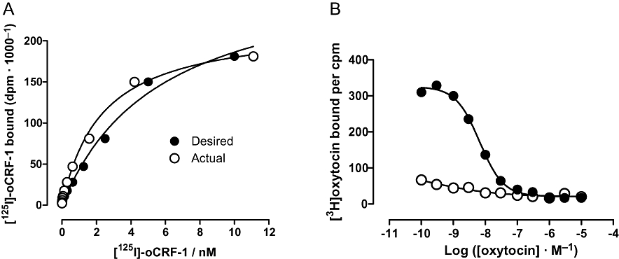
(A) Specific binding of [¹²⁵I]-oCRF to human CRF₁ receptors recombinantly expressed in Chinese hamster ovary (CHO) cells. The filled circles show the data plotted at the desired radioligand concentrations while the open circles show the same binding data plotted at the calculated radioligand concentrations. Lines show the fitted curves. Data from a single experiment are shown. Experiments were performed using a SPA containing 10 µg·mL⁻¹ membrane protein, 5 mg·mL⁻¹ WGA PVT SPA bead and indicated concentrations of [¹²⁵I]oxytocin in a total volume of 100 µL of buffer (50 mM HEPES, 10 mM MgCl₂, 2 mM EDTA, 0.1% bovine serum albumin, 1 µg·mL⁻¹ leupeptin, 1 µg·mL⁻¹ aprotinin, pH 7.4 with KOH). Non-specific binding was determined in the presence of 10 µM rat/human CRF. (B) Competition of human oxytocin for [³H]oxytocin binding at human oxytocin receptors recombinantly expressed in CHO cells. Dilutions of unlabelled oxytocin were prepared using the same tip for the whole set (open circles) or changing the pipette tip after each diluton (filled circles). Experiments were performed using a SPA containing 50 µg·mL⁻¹ membrane protein, 5 mg·mL⁻¹ WGA-coated PVT SPA bead, 1 nM [³H]oxytocin and indicated concentrations of oxytocin in a total volume of 200 µL of buffer (50 mM HEPES, 10 mM MgCl₂, pH 7.4 with KOH). CRF, corticotrophin-releasing factor; PVT, polyvinyl toluene; SPA, scintillation proximity assay; WGA, wheat germ agglutinin.

A more extreme example is shown in Figure 1B. In this case, due to carry over of a ‘sticky’ solution when tips are not changed during the construction of a dilution curve. Competition binding curves to oxytocin against [³H]-oxytocin were constructed, either changing the pipette tip between each dilution or using the same tip for the whole set. The affinity of oxytocin for the ‘tip change’ dilutions agrees very well with the affinity of the radioligand estimated in saturation binding experiments (pK_i= 9.1 cf. pK_D= 9.08 ± 0.07; n= 5). In the no tip change experiment, the affinity of oxytocin appears to be several orders of magnitude greater. Indeed, the effect could almost be described as homeopathic! There is clearly a carry-over phenomenon occurring (perhaps extreme in this case) which is eliminated by changing the tips. Thus, it is clearly a good practice to change tips between dilutions when constructing dilution series. Alternatively, researchers should consider alternatives to serial-dilution and/or the use of non-contact liquid dispensers.

Another potential confounding influence to deriving meaningful data from a fit is in situations where the output of a measurement technology is not linearly related to the pharmacological response. This is the case, for example, for the fluorescence intensity of calcium indicator dyes or the output of technologies which require the analyte concerned to bind to a protein in order to generate the detection signal (e.g. elisa or enzyme complementation-based assays). In each of these cases the signal is (rectangular) hyperbolically related to the concentration of the analyte and fitting the output signal rather than the response distorts the concentration–response curves and may lead to erroneous conclusions – in effect it adds an extra amplification step to the response but one which is irrelevant to the biology that is being investigated. Figure 2 illustrates this for a simulated calcium mobilization experiment using the calcium indicator dye Fluo-4 (Gee et al., 2000). Figure 2A shows a set of simulated calcium mobilizations in cells with a resting cytosolic calcium concentration of 40 nM. These calcium concentrations were then converted to fluorescence intensities as described in the legend to the figure and the corresponding fluorescence intensity changes are plotted in Figure 2B. The most obvious difference between these two sets of data is that the relative maximal effects of the concentration–response curves are distorted by the not calculating the calcium concentrations. When seen as a comparison between agonists this is not particularly concerning as the relative maximal effect of agonists is a system dependent property anyway. However, if we take these curves as representing the effects of an insurmountable antagonist the depression of the maximal response is markedly under-estimated. It should also be noted that while the calcium mobilization concentration–response curves have identical potencies, those of the fluorescence intensity curves differ by approximately fivefold (0.16–0.79) and are all lower than those of the calcium curves. Thus, relative potency is also distorted by not correcting the instrument signal.

Figure 2.

Comparison of concentration–response curves plotted as intracellular calcium concentration (A) or fluorescence intensity (B) from simulated data using the parameters appropriate to the dye Fluo-4 in FLIPR (F_min= 1000, F_max= 77300, K_d= 345 nM). (A) The resting calcium concentration was 40 nM and the peak increases in calcium concentration were 100 nM, 200 nM, 500 nM, 1000 nM and 2000 nM. The midpoint of the concentration–response curves was 1 in each case, the Hill coefficient was also 1. (B) Fluorescence intensities were then calculated using the equation

(transformed from the equation of Grynkiewicz et al., 1985). Symbols for corresponding curves are the same in both graphs. (C) Calcium concentration–response curve with the same maximal response and midpoint but different Hill coeffients (0.5, 0.8, 1, 1.5 and 2). (D) The data in (C) transformed to fluorescence intensities as described above. FLIPR, fluorescent imaging plate reader.

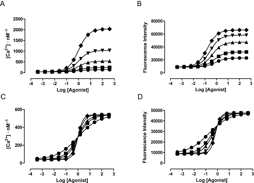
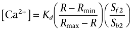
Perhaps counter-intuitively, when the slopes differ between calcium mobilization concentration–response curves, the potencies are distorted but the slopes of the concentration–response curves are preserved when data are analysed as fluorescence intensity (Figure 2C,D). The key point is that not correcting the signal distorts data when the maximal responses or the slopes of the curves differ. Parallel shifts in curves are reported correctly as curves with the same maximal response and slope are distorted in the same way. Thus, any mechanism which results in a change in maximal response or the slope of a concentration–response curve will give an erroneous fit if data are not corrected. Practical solutions to these phenomena could include the use of alternative dyes with lower calcium affinity which will ensure that the response lies on the linear part of the calibration curve. Note, however, that ratiometric dyes (Grynkiewicz et al., 1985) cause the same data distortion as the ‘single wavelength’ dyes when uncalibrated as the calibration equation (3):

(3)

is of the same form as that for single wavelength dyes (equation 4):

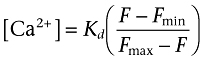(4)

See Grynkiewicz et al. (1985) for the derivation of both equations. Researchers should at least be aware that the choice of detecting dye can have an effect on the resultant dataset.

It should also be remembered that instrument measurements are often ‘counts’ and hence Poisson distributed. Thus, if instrument noise is a dominant source of error in the experiment, the data generated will violate the assumption of Gaussian errors inherent in most non-linear curve fitting algorithms. In this case, the curve fit will need to be weighted (by 1/Y) or an appropriate alternative fitting method will be required.

Continuing with the theme of distortion of concentration–response curves, another confounder to accurate estimation of pharmacological parameters is fitting curves to data pooled from several experimental occasions (H. Giles, unpublished observation). As illustrated in Figure 3, the effect of this is primarily erroneous estimation of the slope of the concentration–response curve. It occurs when the midpoints of the concentration–response curves differ between experimental occasions (irrespective of the behaviour of the maximal response). Thus, while each individual curve has a Hill coefficient of unity the mean of these curves is flat – this is clearly an issue if the model you intend to fit requires a Hill coefficient of unity. Note that there is a distinction to be made here between replicate determinations made on a given experimental occasion and determinations made on separate experimental occasions. The former sample the same underlying concentration–response curve and improve the precision with which it is determined. The latter may well differ from each other in some systematic way due to variations in the underlying concentration–response sampled on each occasion (e.g. because it comes from a different individual). It should therefore be clear that wherever possible a model should be fitted separately to the data derived from each experimental occasion and the separate estimates pooled for statistical comparisons.

Figure 3.

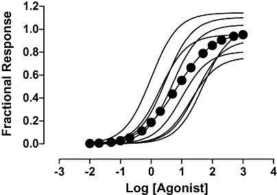
Eight concentration–response curves were simulated with Hill coefficients of 1, random maximal responses which varied between 0.75 and 1.25 and midpoints which varied systematically over the range 1–50. A Hill function was fitted to the data for all eight concentration–response curves and gave a Hill coefficient 0.73. Similar results were obtained whether the maximal response was constant or also varied systematically. Pooling only resulted in a Hill coefficient of unity when the potencies of the pooled curves were identical.

Finally, in this section, we remind readers to be wary of fitting a model when it is unclear that the assumptions of the model derivation are true of the experimental system. An obvious example is ensuring equilibration in binding experiments which are to be analysed using the equations governing binding reactions at equilibrium. It is simply not possible to estimate an equilibrium constant from a saturation or competition binding experiment which has not reached steady state. A widely accepted example of fitting a model whose assumptions are violated by the experimental system is the fitting of a simple two-sited competition model to agonist inhibition binding curves at G-protein-coupled receptors. In this case, the system is known not to contain two independent binding sites for the ligands but a single population of receptor sites whose affinity for the agonist is modulated by the binding of the G-protein. That this is performed knowingly is a partial justification, as at least those working in the field should be familiar with any potential ambiguities in the interpretation of the data. Also, inferences about the relative efficacies of agonists based on their competition curves can be compared with predictions of the model even if the data are not sufficient to allow a direct estimation of the change in affinity of the receptor for the G-protein caused by a given agonist (which is the actual definition of efficacy in the ternary complex model (De Léan et al., 1980).

On the other hand, attempts to measure microscopic equilibrium constants such as receptor isomerization constants (e.g. Claeysen et al., 2000) based on functional experiments using the two state model (Karlin, 1967; Thron, 1972; Colqhoun, 1973) require considerably more caution. The two state model specifically excludes signal transduction processes and is therefore an inappropriate basis for the quantitative analysis of functional data.

Another example of a violation of the assumptions of a model which is not well-justified is a common misuse of homologous competition experiments to estimate the affinity of iodinated peptide radioligands. In many cases (e.g. La Rosa et al., 1992; Van Riper et al., 1993; Neote et al., 1993; Kuestner et al., 1994), the non-iodinated peptide is used as the competing ligand in such an experiment, an approach which suffers from the obvious flaw – the unlabelled ligand is not chemically identical to the radioligand and cannot therefore be assumed to have the same physicochemical or pharmacological properties. This is particularly true for proteins that have been labelled with the Bolton-Hunter reagent (Bolton & Hunter, 1973) as this process condenses a 3-(4-hydroxy, 3-[¹²⁵I]iodophenyl)propanoyl group to free amino groups in the substrate protein. Indeed, even simple iodination of tyrosyl residues can change the binding affinity of a protein. For example, [¹²⁵I]interleukin-8 (IL-8) had a very similar affinity to that of unlabelled IL-8 at human CXCR2 (pK_D= 9.41 ± 0.09, pK_i= 9.27 ± 0.03) but had approximately sixfold higher affinity than IL-8 at CXCR1 (pK_D= 9.64 ± 0.02, pK_i= 8.88 ± 0.03) in a SPA assay using membranes from Chinese hamster ovary (CHO) cells expressing either human receptor (Christopher Browning, unpublished data, n= 3 in all cases). Thus, an affinity for [¹²⁵I]IL-8 derived from a competition experiment with unlabelled IL-8 at CXCR1 will be incorrect as will affinities of competing ligands derived using a Cheng-Prusoff correction based on this affinity. Of course, it would be entirely valid to determine the affinity of cold iodo-IL-8 using homologous competition and use this value in a Cheng-Prusoff correction for competing ligands.

Global fitting

Traditionally, non-linear regression is used on a single set of data, e.g. an agonist concentration response curve or a competition curve in a radioligand binding assay. Global fitting uses non-linear regression to define a family of curves which are analysed simultaneously. The key difference between analysing curves individually and globally is that for the latter, one or more parameters are shared across all of the datasets. This means that for the shared parameter, the curve-fitting program finds a single, global value for all of the datasets. The concept is best illustrated as shown in Figure 4A. The graph shows an agonist concentration–response curve in the presence and absence of a single concentration of a competitive antagonist. The antagonist produces a parallel rightward shift in the agonist curve. Both datasets have been fitted to a three-parameter logistic equation to yield estimates of minimum and maximum asymptotes and pEC₅₀. The 95% confidence intervals of the fits are shown by the dotted lines (you can be 95% sure that the ‘true’ curves lies within these boundaries). It is clear that the confidence intervals are quite wide, especially for the minimum asymptote of the control curve and the maximum asymptote of the curve in the presence of the antagonist. This is not surprising – closer inspection of the datasets shows that these parameters are poorly defined by the datasets. The definition of the maxima and minima of the curves are crucial to estimating the midpoint i.e. the pEC₅₀. While the fitted pEC₅₀ value for the control curve is 6.3, the 95% confidence interval is 5.8 to 6.9, spanning over a log unit.

Figure 4.

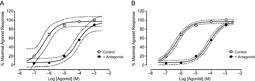
Individual (A) or global (B) fits of control and antagonist-treated concentration–response curves according to a three-parameter logistic equation. 95% confidence intervals of the fitted curves are shown using dashed lines.

However, it should be noticed that the control curve defines the maximal agonist response very well and that the antagonist-treated curve defines the minimum response equally well. What if global fitting were to be used? Analysis according to the same three-parameter logistic equation but with shared values for the maximal and minimal asymptotes is shown in Figure 4B. It is clear that the improved definition of the asymptotes has greatly reduced the 95% confidence intervals, which in turn reduces the error on the estimated pEC₅₀ values. The 95% confidence interval for the pEC₅₀ value for the control curve using the global fit is 6.2 to 6.5, much tighter than for the individual fit in Figure 4A. This is in part due to the better definition of the minimum and maximum asymptotes, but also due to the increased degrees of freedom of the resulting global fit (due to more data points being included in the fit).

It should be noted that there are some simple, but important requirements for global fitting. First, it is assumed that all datasets being fitted globally have the same degree of scatter – it is not meaningful to analyse one curve that has very little scatter in conjunction with a second which has a large amount of scatter. Second, it is crucial that the units for both curves are the same – global fitting will not work if one curve is expressed as ‘% maximal agonist response’ and others are in ‘relative fluorescence units’, for example.

The example above shows the utility of global fitting to improve the fidelity of parameter estimates for incomplete datasets. However, the most powerful aspect of global fitting is to directly fit models which cannot be used for single datasets alone. The first example of such a model is Schild analysis for competitive antagonists (Arunlakshana and Schild, 1959). Classical determination of competitive antagonist affinity studies the effects of multiple, fixed antagonist concentrations on an agonist concentration–response curve. Increasing antagonist concentrations (theoretically) produce a parallel rightward shift in the agonist curve. This is quantified by measuring the degree of shift (concentration-ratio) for each antagonist concentration with respect to the control curve. The logarithm of the (concentration-ratio – 1) is then plotted against the logarithm of antagonist concentration to yield a Schild regression. For a competitive antagonist the slope of the regression should be not significantly different from one (and constrained as such if so). The intercept on the X-axis is equal to the logarithm of the equilibrium dissociation constant for the antagonist, K_B. This method is widely used, yet has flaws which can make it unsuitable for some assay designs and can also lead to error in the estimation of the antagonist affinity.

For example, if the assay system in use does not permit multiple curves to be generated, e.g. because of receptor internalization, then it is not possible to calculate intra-assay concentration-ratios. A further issue with the Schild method is the over-reliance on the control agonist curve. Each calculation of a concentration-ratio requires reference to the control curve and one other curve to generate the Schild regression. This places a greater weight on the control agonist curve than on the other datasets; any error in the estimation of agonist EC₅₀ is perpetuated in the estimation of antagonist affinity, especially if the EC₅₀ is underestimated (Lew and Angus, 1995). For similar reasons, it is no longer considered best practice to use a Scatchard transformation to analyse saturation binding data; therefore, why should it be acceptable to do the same for Schild analysis?

Figure 5 shows the analysis of a dataset using both traditional linear regression (A) and non-linear global fitting (B) for pirenzepine antagonizing the effect of methacholine at the human muscarinic M₃ receptor. In the latter, data are fitted globally according to the Schild equation (5) to find shared values that best describe the EC₅₀ of the control curve, the maximum and minimum asymptotes, the Hill slope, the pA₂ value and the Schild slope.

Figure 5.

(A) Classical Schild analysis of pirenzepine-mediated antagonism of methacholine-stimulated calcium mobilization at the muscarinic M₃ receptor. From four parameter logistic fits of the curves (with a common Hill slope), concentration-ratios with respect to the control curve are calculated and plotted against the antagonist concentration to yield a Schild regression. The X-intercept of the regression represents the pA₂ value for pirenzepine. (B) Global fit of the same dataset to the Schild equation to find shared values for EC₅₀ of the control curve, the maximum and minimum asymptotes, the Hill slope, the pA₂ value and the Schild slope. Parameter estimates, errors and 95% confidence intervals are shown in the table.

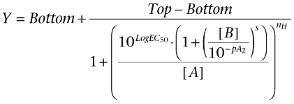(5)

Note that the analysis provides the same parameters that are obtained from a traditional method without the need for linear regression (i.e. pA₂ value and Schild slope). These parameters can be interpreted in exactly the same manner as previously i.e. if the Schild slope is not significantly different to unity, then it can be constrained as such and the pA₂ value equals the pK_B. For the example in Figure 5A, the estimate for pA₂ is 7.79 with a 95% confidence interval of 7.60 to 8.02 for the linear Schild regression. For the non-linear fit, the estimated pA₂ is 8.02 with a 95% confidence interval of 7.86 to 8.17 (Figure 5B). This interval is narrower than that achieved using linear regression, highlighting the improved accuracy of the global fitting method. We note in writing this review that for good datasets which obey the rules of purported competitive antagonism (concentration-dependent, parallel rightward shifts of an agonist curve), the difference between the two methods is generally negligible in terms of output. However, for datasets which result in more scattered Schild regressions, global analysis will produce a much more accurate estimation of antagonist affinity.

Finally, despite arguing that global fitting is a superior method for performing Schild analysis compared with the null method approach, there is still great value in calculating and plotting a Schild regression. In the same way that deviations from linearity in a Scatchard plot can indicate behaviour inconsistent with single-site binding, visualizing non-linearity in a Schild regression can alert the experimenter to a different mechanism of antagonist action or non-equilibrium conditions. Therefore, the best approach is to determine the parameter estimates (pA₂, Schild slope, etc.) by global fitting, but to also plot a Schild regression to enable greater interrogation of the data.

A further example of the use of global fitting where single curve fitting is not possible is for the measurement of partial agonist efficacy using the operational model of agonism described by Black and Leff (1983). It is not the intention of this review to discuss the model in depth as it has been extensively described in the literature (Motulsky and Christopoulos, 2004; Kenakin, 2009). However, some understanding of the model is required to understand the benefits of using global fitting. The operational model recognizes that the potency of an agonist (as measured by its EC₅₀) is actually a composite of two parameters – namely affinity and efficacy. The former is described by an equilibrium dissociation constant, K_A, which is invariant to the agonist-receptor pair. However, it is well known that an agonist can show vastly different potencies at a given receptor, depending on factors such as receptor expression (Wilson et al., 1996; Kenakin, 2009). If the affinity of an agonist for the receptor is unchanged, then it must be differences in efficacy that are responsible for the difference in potencies. (It should be noted at this point that many pharmacologists believe that agonist affinity and efficacy are intrinsically linked (Strange, 2008). If this is the case, not only would efficacy vary when measuring an agonist's activity at multiple pathways, but rather K_A could equally be different for different receptor conformations. However, for the purposes of this example, it is easier to assume that K_A is invariant for an agonist-receptor pair).

Efficacy in the operational model is described using the parameter, τ (tau). This is often the subject of much confusion as it is a theoretical term without units - a common question regarding τ is ‘what does it actually mean?’. In strict terms, it is the ratio of receptor expression level to the concentration of agonist-receptor complex that produces a half-maximal stimulus. However, while meaningful, it is not a particularly useful intrinsic value as it is system dependent. However, τ is a useful parameter for the relative quantification of agonist efficacies. Values of τ must be interpreted carefully as a number of factors contribute to observed potency: (i) the level of receptor expression; (ii) the signal amplification between the receptor and the assay endpoint; and (iii) the intrinsic ability of the agonist to activate the receptor and produce a stimulus (i.e. the agonist's intrinsic efficacy). It is point (iii) that pharmacologists are generally concerned with when thinking about the concept of agonist efficacy, but the influence of points (i) and (ii) should not be forgotten. For this reason, it is possible to compare τ values for different agonists at the same receptor in the same assay (as both receptor expression and signal amplification will be the same). Alternatively, it is possible to compare τ values for the same agonist in different assay formats (where the intrinsic efficacy will be unchanged with varying receptor expression/signal amplification).

The operational model is expressed in equation form as shown in Figure 6A. Unlike the four-parameter logistic equation (Figure 6B) that would ordinarily be used for an agonist concentration–response curve, the operational model has five parameters: The agonist equilibrium dissociation constant (K_A), the response in the absence of agonist (Basal), the maximum possible system response (Effect_Max), the agonist efficacy (τ) and the slope of the transducer function linking occupancy to response (n). But if the equation is not much more complex than a four-parameter logistic fit, why is global fitting required? The problem is that the operational model has more parameters (five) than are required to fully define a single concentration–response curve (four). Therefore, an infinite combination of parameters could actually fit the dataset for a single agonist curve, rendering the estimates meaningless. Essentially changes in one parameter which increase the sum-of-squares (worsen the fit) can be offset by compensatory changes in the other parameters when the model has too many parameters. This can be resolved by using global fitting: Including further curves into the model fit provides extra constraints which allow the fitting algorithm to identify optimal parameters less ambiguously.

Figure 6.

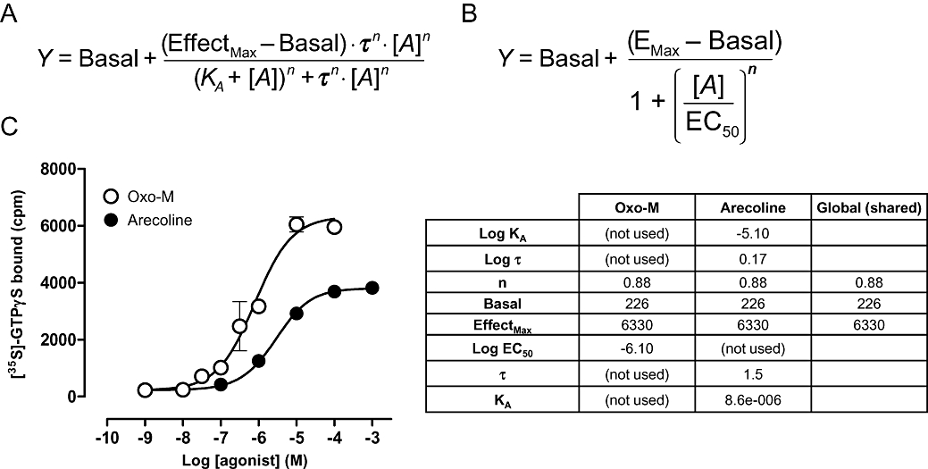
Equations for the operational model of agonism (A) and a four parameter logistic fit (B). Direct fitting of the operational model for a partial agonist (arecoline) using global fitting (C). Estimates of Basal, Effect_Max and transducer slope (n) are derived from a four-parameter fit of the full agonist (oxotremorine-M) curve. Estimates of affinity (K_A) and efficacy (τ) of arecoline are shown in the table.

Figure 6C shows the partial agonist effect of arecoline to stimulate [³⁵S]GTPγS binding via the G_q/11 subunit at the human muscarinic M₁ acetylcholine receptor expressed in CHO cells. Also shown is the analysis according to the operational model to generate estimates of affinity and efficacy. The key to this analysis is that the partial agonist curve must be analysed globally in conjunction with a curve to a full agonist, in this case, oxotremorine-M. The method works because for a full agonist, the estimates of Basal, E_max and Hill slope from a four-parameter fit are actually very close to the values of Basal, Effect_max and transducer slope (n), respectively, in the operational model. Thus, fitting the curve for the full agonist to a four-parameter logistic fit yields values for three of the five parameters of the operational model. By sharing these three key parameter estimates across both datasets, it is then easy to fit the curve for the partial agonist to the operational model to generate estimates of the remaining parameters, K_A and τ. In this example, analysis of the arecoline dataset suggests an equilibrium dissociation constant, K_A= 8.6 µM and τ= 1.5. Note that it is not possible to resolve the affinity and efficacy of a full agonist using this method. To generate such data requires either assays under different degrees of permanent receptor inactivation or, more simply, independent determination of agonist affinity, e.g. in a radioligand binding assay. This value can then be fed into the operational model to generate estimates of full agonist efficacy.

Finally, it should be mentioned that there are drawbacks to globally fitting datasets. As the number of parameters that are able to be fitted increase, so the complexity of the fitting processes itself increases. It is not uncommon for non-linear regression with complex models (such as those used in the analysis of allosteric modulation, for example) to find local minina in the iterative process. Thus, the increased power of global fitting comes with the need for the experimenter to provide reasonably accurate initial values for the parameters in the fit, in order to avoid potential local minima and hence errant data.

‘Is it significantly different?’

Statistics is an area that can be difficult for researchers whose only memory from their degree or PhD is how to do a t-test! However, it is commonplace for questions to be asked of receptor pharmacology datasets which require knowledge of relevant statistics: Is the Schild slope significantly different from unity? Is the EC₅₀ for an agonist changed after treatment of the cells/tissue? Does a one-site or two-site model fit the radioligand binding data better? In this section the use of statistics to answer such questions will be discussed. This section is not intended to be comprehensive, but rather to introduce some simple concepts that those working in receptor pharmacology may find useful. Readers with further questions are advised to consult the extensive literature in this area (Motulsky, 1995; Motulsky and Christopoulos, 2004; Kenakin, 2009).

All of the example questions above require some form of comparison between two data fits to be performed. However, before even considering any form of comparison, some simple questions should be addressed. Do both the model fits that you want to compare adequately and reasonably fit the data? If, despite numerous attempts, a dataset cannot be fitted using a given model, then it is fairly safe to assume that the model is not correct and a comparison is unnecessary. If both models appear to fit the data, but for one or both of the fits the parameter estimates make no sense then again, you must question whether the model is suitable. It may be that the dataset you have analysed is insufficiently powered in terms of number of data points or replicates for the analysis. Alternatively the model may simply be inappropriate. If both models fit the data well then a comparison between the two may be valid.

Typically, the goodness of fit of a model to a dataset is measured by the sum of the squares of the vertical difference between the data points and the fitted regression. However, it is often observed that the fit with the lowest sum of squares is not necessarily the preferred fit. Why could this be? A two-site binding model, by virtue of its increased number of parameters, will inevitably have more flexibility to fit a competition binding curve than a one-site model – it does not necessarily mean that it describes the data better. Some kind of further comparison which accounts for this added flexibility is required. Most often the comparison is being made between two models of which one will be a simpler version of the other, e.g. a one-site versus two-site binding model. As these models are related, but merely differ in complexity, they are said to be nested. There are two ways of comparing such models – statistical hypothesis testing or information theory.

In statistical hypothesis testing the models must be nested in order to perform the analysis, called an extra-sum-of-squares F-test. A null hypothesis is formed, in this case that the simpler model is correct. Recognizing that it is insufficient to simply compare the sum of squares for two model fits, the F-test takes into account the number of data points and number of parameters for each model (hence the name extra-sum-of-squares). An F-ratio is generated, from which a P-value can be derived (the derivation of the model and calculation of F-ratios and P-values is well-described elsewhere; Motulsky, 1995). The F-ratio is calculated as follows:

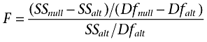(6)

Where SS_null and SS_altare the sum-of-squares for the null and alternative (more complex) model fits, respectively, and Df_null and Df_alt are the degrees of freedom for the model fits respectively. The P-value is calculated from the F-ratio (and Df values) using the F-distribution and is commonly performed automatically in curve-fitting software. Alternatively, it can be performed using tables or as a function in Excel.

Once analysed, if the P-value is small, then it means that either the more complex model must be correct or that the simpler model is correct, but by chance the more complicated model happened to fit better on this test occasion. In order to decide whether one model is significantly better than another, an arbitrary level of significance must be assigned. Usually this is set at 5%, such that a P-values less than 0.05 represent situations where the experimenter is happy to accept that the more complicated model represents a significantly better fit. It must be noted that it is the experimenter's responsibility to set the level of significance as appropriate for the study in question.

How does this work in practice? Continuing the example of Schild analysis from earlier, a Schild slope of unity is an indicator of competitive antagonism, whereas deviation from unity can suggest an alternative mechanism. How do you determine whether a Schild slope is significantly different from one? Taking the example from Figure 5, it is necessary to analyse the dataset globally according to the Schild equation with the slope value constrained to 1 and also unconstrained and then perform a comparison of the two fits. Performing this analysis for the data in Figure 5B shows that there is a lower sum-of-squares for the fit with the Schild slope unconstrained (18 446) compared with the fit with the slope value constrained to 1 (20 340). However, there will be a difference in the degrees of freedom between the two fits as there will be a difference between the numbers of parameters to be fitted. Taking this into account yields an F-ratio of 8.212, which translates to P= 0.005; suggesting that the improvement in fit observed by leaving the Schild slope unconstrained more than compensates for the increased degree of freedom associated with fitting this extra parameter. Therefore, we should reject the null hypothesis and accept the more complex model where the Schild slope is unconstrained in this experiment.

In this example, the difference from unity is actually relatively small and would result in very little difference between the pA₂ value and the pK_B value were the slope to be constrained to one. In practice you would repeat the experiment several times, estimate the Schild slope for each experiment and test the mean of the log of these slopes against zero to determine whether the slope value was significantly different to unity. However, the utility of being able to test whether the Schild slope is significantly different to unity for individual experiments is useful and may serve as an indicator to an experimenter of competitive behaviour or otherwise.

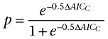
An alternative method for comparing two fits to a single dataset is to use Akaike's Information Criterion (AIC). It is not based on hypothesis testing, so does not require a null hypothesis or P-values. Also, it does not require that the two models being compared are nested (although for these purposes they usually are). AIC uses information theory to compare two different models to (i) estimate which model is more likely to be correct; and (ii) quantify how much more likely it is to be correct. As with the F-test above, the derivation and theory of AIC will not be discussed in this review, but can be found elsewhere (Burnham and Anderson, 2002; Motulsky and Christopoulos, 2004). However, the essence of the comparison is similar: AIC enables comparison of two models by comparing the sum-of-squares and taking into account the difference in the complexity as determined by the difference in the number of parameters. An AIC value (or, more appropriately for ‘small’ datasets, a correctedAIC value, AIC_C) is calculated for both fits and it is the difference in AIC_C that determines which of the two models is more likely to be correct; the model with the lower AIC_C value is the more likely. The probability that a model is correct is governed by the following equation:

(7)

where ΔAIC_C is the change in AIC_C value. If the values are identical for the two fits, then there is no evidence to favour one fit above the other i.e. both are equally likely. However, if one model were to have an AIC_C value of 4.0 less than another model, then the probability that it is correct would be 88%. To use the same example of Schild analysis as above, the difference in AIC_C between fits with the Schild slope constrained to one and unconstrained is 6.03, suggesting that the probability that the latter fit is correct is 95.3%. As with the F-test above, this is only meaningful if the models that have been chosen are sensible in the first place. If you do not have a sufficiently powered dataset to fit a complex model, then comparison of such a model with a simpler model will almost inevitably result in a preference for the latter.

The major difference of AIC compared with the more common statistical hypothesis testing is that the onus is greater on the experimenter with AIC. There is no measure of significance, only a measure of likelihood in the form of a ratio of probabilities. A very large change in AIC_C value points strongly to one model in preference to another; a very small change makes such a conclusion more uncertain. You can choose to accept the simpler model unless the more complex model is much more likely. If the results are equivocal, then you can accept the results of the AIC anyway or conclude that the data are ambiguous and that further experimentation may be required. Either way, rather than drawing an arbitrary ‘line in the sand’, which is often the case for statistical hypothesis testing, AIC forces the experimenter to think about their results.

Summary

The range of assays and technologies now available to the pharmacologist is incredibly diverse. With this increase in technology and the subsequent ‘industrialization’ of pharmacology, less thought is given to principles of good experimental design. Indeed, a cynic might argue that we now design experiments around the capabilities of our machines rather than designing our machines to perform the experiments we want to do. It is also arguably the case that recent improvements in processing power and the apparent ease with which complex pharmacological models can applied within software packages, distances the researcher from the underpinning mathematical and pharmacological understanding.

In this article we have addressed experimental design issues such as the dilution range of compounds required to accurately define parameters. We have also examined the effect of dilution fidelity, the relationship between a cellular response and instrument measurement and the effect of pooling data from across experiments on the results obtained. These examples demonstrate the importance of understanding the experimental design and the factors which can influence or distort the output.

In the second part of the review, we have considered methods of data analysis. Of particular note is the utility of global fitting which is available as a result of the evolution of scientific curve-fitting software. Global fitting enables pharmacologists to improve their current methods, e.g. for Schild analysis or to directly analyse datasets that were not possible to analyse without global fitting, e.g. operational modelling of partial agonist function. Finally, this article reviews statistical analysis of receptor pharmacology datasets and the applicability of both statistical hypothesis testing and information theory to situations commonly encountered when analysing data, although this has largely been in terms of the quality of curve fits and inference from single datasets rather than analysis of the data from a set of replicate experiments.

We hope that in highlighting these issues, scientists actively engaged in running receptor assays can engage (or re-engage) with the pharmacological principles described above to improve both their own understanding and the quality of data that they produce.

Glossary

Abbreviations

AIC

Akaike's Information Criterion

CHO

Chinese hamster ovary

CRF

corticotrophin-releasing factor

GTP(gamma)S

guanosine 5′-O-[gamma-thio]triphosphate

PVT

polyvinyl toluene

SPA

scintillation proximity assay

Conflict of interest

The authors have no conflict of interest to declare.

References

- Arunlakshana O, Schild HO. Some quantitative uses of drug antagonists. Br J Pharmacol. 1959;14:48–58. doi: 10.1111/j.1476-5381.1959.tb00928.x. [DOI] [PMC free article] [PubMed] [Google Scholar]
- Black JW, Leff P. Operational models of pharmacological agonism. Proc R Soc Lond B Biol Sci. 1983;220:141–162. doi: 10.1098/rspb.1983.0093. [DOI] [PubMed] [Google Scholar]
- Bolton AE, Hunter WM. Labelling of proteins to high specific radioactivities by conjugation to a 125I-containing acylating agent. Biochem J. 1973;133:529–539. doi: 10.1042/bj1330529. [DOI] [PMC free article] [PubMed] [Google Scholar]
- Burnham KP, Anderson DR. Model Selection and Multimodel Inference: A Practical Information-Theoretic Approach. New York: Springer-Verlag; 2002. [Google Scholar]
- Chang K-J, Jacobs S, Cuatrecasas P. Quantitative aspects of hormone receptor interactions of high affinity: effect of receptor concentration and measurement of dissociation constants of labelled and unlabelled hormones. Biochim Biophys Acta. 1975;406:294–303. doi: 10.1016/0005-2736(75)90011-5. [DOI] [PubMed] [Google Scholar]
- Christopoulos A. Assessing the distribution of parameters in models of ligand-receptor interactions: to log or not to log. Trends Pharmacol Sci. 1998;19:351–357. doi: 10.1016/s0165-6147(98)01240-1. [DOI] [PubMed] [Google Scholar]
- Claeysen S, Sebben M, Bécamel C, Eglen RM, Clark RD, Bockaert J, et al. Pharmacological properties of 5-hydroxytryptamine4 receptor antagonists on constitutively active wild-type and mutated receptors. Molec Pharmacol. 2000;58:136–144. doi: 10.1124/mol.58.1.136. [DOI] [PubMed] [Google Scholar]
- Colqhoun D. The relation between classical and cooperative models for drug action. In: Rang HP, editor. Drug Receptors. London: The Macmillan Company; 1973. pp. 149–182. [Google Scholar]
- De Léan A, Stadel JM, Lefkowitz RJ. A ternary complex model explains the agonist-specific binding properties of the adenylate cyclase coupled β-adrenergic receptor. J Biol Chem. 1980;255:7108–7117. [PubMed] [Google Scholar]
- Gee KR, Brown KA, Chen W-NU, Bishop-Stewart J, Gray D, Johnson I. Chemical and physiological characterisation of fluo-4 Ca2+-indicator dyes. Cell Calcium. 2000;27:97–106. doi: 10.1054/ceca.1999.0095. [DOI] [PubMed] [Google Scholar]
- Goldstein A, Barrett RW. Ligand dissociation constants from competition binding assays: errors associated with ligand depletion. Mol Pharmacol. 1987;31:603–609. [PubMed] [Google Scholar]
- Grynkiewicz G, Poenie M, Tsien RY. A new generation of Ca2+ indicators with greatly improved fluorescence properties. J Biol Chem. 1985;260:3440–3450. [PubMed] [Google Scholar]
- Hall DA. Modelling the functional effects of allosteric modulators at pharmacological receptors: an extension of the two state model of receptor activation. Molec Pharmacol. 2000;58:1412–1423. doi: 10.1124/mol.58.6.1412. [DOI] [PubMed] [Google Scholar]
- Hulme EC, Birdsall NJM. Strategy and tactics in receptor binding studies. In: Hulme EC, editor. Receptor-Ligand Interactions: A Practical Approach. Oxford: Oxford University Press; 1992. pp. 63–176. [Google Scholar]
- Karlin A. On the application of ‘a plausible model’ of allosteric proteins to the receptor for acetylcholine. J Theor Biol. 1967;16:306–320. doi: 10.1016/0022-5193(67)90011-2. [DOI] [PubMed] [Google Scholar]
- Kenakin TP. A Pharmacology Primer. London: Elsevier; 2009. [Google Scholar]
- Kuestner RE, Elrod RD, Grant FJ, Hagen FS, Kuijper JL, Matthews SL, et al. Cloning and characterisation of an abundant subtype of the human calcitonin receptor. Molec Pharmacol. 1994;46:246–255. [PubMed] [Google Scholar]
- La Rosa GJ, Thomas KM, Kaufmann ME, Mark R, White M, Taylor L, et al. Amino terminus of the IL-8 receptor is the major determinant of receptor subtype specificity. J Biol Chem. 1992;267:25402–25406. [PubMed] [Google Scholar]
- Lew MJ, Angus JA. Analysis of competitive agonist–antagonist interactions by nonlinear regression. Trends Pharmacol Sci. 1995;16:328–337. doi: 10.1016/s0165-6147(00)89066-5. [DOI] [PubMed] [Google Scholar]
- Motulsky H. Intuitive Biostatistics. New York: Oxford University Press; 1995. [Google Scholar]
- Motulsky H, Christopoulos A. Fitting Models to Biological Data Using Linear and Non-Linear Regression: A Practical Guide to Curve Fitting. New York: Oxford University Press; 2004. [Google Scholar]
- Neote T, Darbonne W, Ogez J, Horuk R, Schall TJ. Identification of a promiscuous inflammatory peptide binding site on the surface of red cells. J Biol Chem. 1993;268:12247–12249. [PubMed] [Google Scholar]
- Paton WDM, Rang HP. A kinetic approach to the mechanism of drug action. In: Harper NJ, Simmonds AB, editors. Advances in Drug Research. New York: Academic Press; 1966. pp. 57–80. [Google Scholar]
- Strange PG. Agonist binding, agonist affinity and agonist efficacy at G protein-coupled receptors. Br J Pharmacol. 2008;153:1353–1363. doi: 10.1038/sj.bjp.0707672. [DOI] [PMC free article] [PubMed] [Google Scholar]
- Swillens S. Interpretation of binding curves obtained with high receptor concentrations: practical aid for computer analysis. Mol Pharmacol. 1995;47:1197–1203. [PubMed] [Google Scholar]
- Thron CD. On the analysis of pharmacological experiments in terms of an allosteric model. Molec Pharmacol. 1972;9:1–9. [PubMed] [Google Scholar]
- Van Riper G, Siciliano S, Fischer PA, Meurer R, Springer MS, Rosen H. Characterisation and species distribution of high affinity GTP-coupled receptors for human Rantes and monocyte chemoattractant protein 1. J Exp Med. 1993;177:851–856. doi: 10.1084/jem.177.3.851. [DOI] [PMC free article] [PubMed] [Google Scholar]
- Wilson S, Chambers JK, Park JE, Ladurner A, Cronk DW, Chapman CG, et al. Agonist potency at the cloned human beta-3 adrenoceptor depends on receptor expression level and nature of assay. J Pharmacol Exp Ther. 1996;279:214–221. [PubMed] [Google Scholar]