On the Bumpy Road to the Dominant Mode

Abstract

Maximum likelihood estimation in many classical statistical problems is beset by multimodality. This article explores several variations of deterministic annealing that tend to avoid inferior modes and find the dominant mode. In Bayesian settings, annealing can be tailored to find the dominant mode of the log posterior. Our annealing algorithms involve essentially trivial changes to existing optimization algorithms built on block relaxation or the EM or MM principle. Our examples include estimation with the multivariate t distribution, Gaussian mixture models, latent class analysis, factor analysis, multidimensional scaling and a one-way random effects model. In the numerical examples explored, the proposed annealing strategies significantly improve the chances for locating the global maximum.

1. Introduction

Multimodality is one of the curses of statistics. The conventional remedies rely on the choice of the initial point in iterative optimization. It is a good idea to choose the initial point to be a suboptimal estimate such as a method of moments estimate. Unfortunately, this tactic does not always work, and statisticians turn in desperation to multiple random starting points. The inevitable result is an inflation of computing times with no guarantee of success.

In combinatorial optimization, simulated annealing often works wonders (Metropolis et al., 1953; Kirkpatrick et al., 1983; Press et al., 1992). This fruitful idea from statistical physics also applies in continuous optimization, but it still entails an enormous number of evaluations of the objective function. In a little noticed paper, Ueda & Nakano (1998) adapt simulated annealing to deterministic estimation in admixture models. In modifying the standard expectation maximization (EM) algorithm for admixture estimation, they retain the annealing part of simulated annealing and drop the simulation part. Annealing operates by flattening the likelihood surface and gradually warping the substitute surface towards the original surface. By the time all of the modes reappear, the iterates have entered the basin of attraction of the dominant mode.

In this article, we explore several variations of deterministic annealing. All of these involve surface flattening and warping. A tuning parameter controls the process of warping a relatively flat surface with a single or handful of modes into the ultimate bumpy surface of the objective function. Our constructions are admittedly ad hoc and tailored to specific problems. Consequently, readers expecting a coherent theory are apt to be disappointed. In our defense, these problems have resisted solution for a long time, and it is unrealistic to craft an overarching theory until we better understand the nature of the enemy. Readers with a mathematical bent will immediately recognize our debt to homotopy theory in topology and central path following in convex optimization.

We specifically advocate four different tactics: (i) degrees of freedom inflation, (ii) noise addition, (iii) admixture annealing, and (iv) dimension crunching. Each of these techniques compares favourably with multiple random starts in a concrete example. In some cases, the intermediate functions constructed in annealing no longer bear a statistical interpretation. This flexibility should be viewed as a positive rather than a negative. We focus on EM algorithms (Dempster et al., 1977; McLachlan & Krishnan, 2008), the closely related MM algorithms (de Leeuw, 1994; Heiser, 1995; Becker et al., 1997; Lange et al., 2000; Hunter & Lange, 2004; Wu & Lange, 2008) and block relaxation algorithms (de Leeuw, 1994) because they are easy to program and consistently drive the objective function uphill or downhill. In our examples, the standard algorithms require only minor tweaking to accommodate annealing. The MM algorithm has some advantages over the EM algorithm in the annealing context as MM algorithms do not require surrogate functions to be likelihoods or log-likelihoods.

Our examples rely on a positive tuning parameter ν attaining an ultimate value ν^∞ defining the objective function. The initial ν⁰ starts either very high or low. When ν^∞ is finite, after every s iterations we replace the current value νⁿ of ν by νⁿ⁺¹ = rνⁿ + (1 – r)ν^∞ for r ∈ (0, 1). This construction implies that νⁿ converges geometrically to ν^∞ at rate r. When ν^∞ is infinite, we take ν⁰ positive, r > 1 and replace νⁿ by νⁿ⁺¹ = rνⁿ. The value of the update index s varies with the application.

Our examples include: (i) estimation with the t distribution, (ii) Gaussian mixture models, (iii) latent class analysis, (iv) factor analysis, (v) multidimensional scaling, and (vi) a one-way random effects model. Example (vi) demonstrates the relevance of annealing to maximum a posteriori estimation. These well-known problem areas are all plagued by the curse of multimodality. Eliminating inferior modes is therefore of great interest. Our first vignette on the t distribution is designed to help the reader visualize the warping effect of annealing. Before turning to specific examples, we briefly review the MM algorithm.

2. MM algorithm

The MM algorithm (de Leeuw, 1994; Heiser, 1995; Becker et al., 1997; Lange et al., 2000; Hunter & Lange, 2004; Wu & Lange, 2009), like the EM algorithm, is a principle for creating algorithms rather than a single algorithm. There are two versions of the MM principle. In maximization the acronym MM stands for iterative minorization-maximization; in minimization it stands for majorization-minimization. Here we deal only with the maximization version. Let f(θ) be the objective function we seek to maximize. An MM algorithm involves minorizing f(θ) by a surrogate function g(θ|θⁿ) anchored at the current iterate θⁿ of a search. Minorization is defined by the two properties

$$f\left({\theta }^n\right)=g({\theta }^n\mid {\theta }^n)$$ (1)

$$f\left(\theta \right)\ge g(\theta \mid {\theta }^n),\theta \ne {\theta }^n.$$ (2)

In other words, the surface $\theta \mapsto g(\theta \mid {\theta }^n)$ lies below the surface $\theta \mapsto f\left(\theta \right)$ and is tangent to it at the point θ = θⁿ. Construction of the minorizing function g(θ|θⁿ) constitutes the first M of the MM algorithm.

In the second M of the algorithm, we maximize the surrogate g(θ|θⁿ) rather than f(θ). If θⁿ⁺¹ denotes the maximum point of g(θ|θⁿ), then this action forces the ascent property f(θⁿ⁺¹) ≥ f(θⁿ). The straightforward proof

$$f\left({\theta }^{n+1}\right)\ge g({\theta }^{n+1}\mid {\theta }^n)\ge g({\theta }^n\mid {\theta }^n)=f\left({\theta }^n\right),$$

reflects definitions (1) and (2) and the choice of θⁿ⁺¹. The ascent property is the source of the MM algorithm's numerical stability. Strictly speaking, it depends only on increasing g(θ|θⁿ), not on maximizing g(θ|θⁿ). The art in devising an MM algorithm revolves around intelligent choices of minorizing functions and skill with inequalities.

3. Multivariate t distribution

The multivariate t distribution is often employed as a robust substitute for the normal distribution in data fitting (Lange et al., 1989). For location vector $\mu \in {\mathbb{R}}^p$, a positive definite scale matrix $\Omega \in {\mathbb{R}}^{p\times p}$ and degrees of freedom α>0, the multivariate t distribution has density

$$f\left(x\right)=\frac{\Gamma \left(\frac{\alpha +p}{2}\right)}{\Gamma \left(\frac{\alpha }{2}\right){\left(\alpha \pi \right)}^{p∕2}{\mid \Omega \mid }^{1∕2}{[1+\frac{1}{\alpha }{(x-\mu )}^t{\Omega }^{-1}(x-\mu )]}^{(\alpha +p)∕2}},x\in {\mathbb{R}}^p.$$

Maximum likelihood estimation of the parameters μ and Ω for fixed α is challenging because the likelihood function can exhibit multiple modes. Values of α below 1 are particularly troublesome. The standard EM algorithm (Lange et al., 1989) updates are

$$\begin{array}{cc}\hfill {\mu }^{n+1}& =\frac{1}{v^n}\sum _{i=1}^m{w}_i^n{x}_i,\hfill \\ \hfill {\Omega }^{n+1}& =\frac{1}{m}\sum _{i=1}^m{w}_i^n(x_i-{\mu }^{n+1}){(x_i-{\mu }^{n+1})}^t,\hfill \end{array}$$

where the superscripts n and n+1 indicate iteration number, m is the sample size, and $v^n={\sum }_{i=1}^m{w}_i^n$ is the sum of the case weights

$$w_i^n=\frac{\alpha +p}{\alpha +d_i^n},d_i^n={(x_i-{\mu }^n)}^t{\left({\Omega }^n\right)}^{-1}(x_i-{\mu }^n).$$

An alternative faster algorithm (Kent et al., 1994; Meng & van Dyk, 1997) updates Ω by

$${\Omega }^{n+1}=\frac{1}{v^n}\sum _{i=1}^m{w}_i^n(x_i-{\mu }^{n+1}){(x_i-{\mu }^{n+1})}^t.$$

We will use this faster EM algorithm in the subsequent numerical examples. When estimating μ with both Ω and α fixed, one simply omits the Ω updates.

There are two strategies for flattening the likelihood surface. The first involves degree of freedom inflation. As α tends to ∞, the score function for the location parameter μ tends to the normal score with a single root equal to the sample mean. EM annealing substitutes ν for α, starts with a large value of ν, and works its way down to ν^∞ = α. As the iterations proceed, the EM iterates migrate away from the sample mean towards the dominant mode.

The second annealing strategy adds noise. Given m independent observations x₁,..., x_m, the log-likelihood is

$$\ln L(\mu ,\Omega )=-\frac{m}{2}\ln \mid \Omega \mid -\frac{\alpha +p}{2}\sum _{i=1}^m\ln [\alpha +{(x_i-\mu )}^t{\Omega }^{-1}(x_i-\mu )]+c,$$

where c is an irrelevant constant. In annealing, we maximize the modified log-likelihood

$$\ln L(\mu ,\Omega ,v)=-v\frac{m}{2}\ln \mid \Omega \mid -\frac{\alpha +p}{2}\sum _{i=1}^m\ln [\alpha +{(x_i-\mu )}^t{\Omega }^{-1}(x_i-\mu )]+c.$$

Taking the positive tuning constant ν<1 flattens the likelihood surface, while taking ν>1 sharpens it. Under annealing, the standard EM algorithm updates Ω by

$${\Omega }^{n+1}=\frac{1}{vm}\sum _{i=1}^m{w}_i^n(x_i-{\mu }^{n+1}){(x_i-{\mu }^{n+1})}^t.$$ (3)

Following the derivation of the alternative EM algorithm in Wu & Lange (2008), one can demonstrate with effort that the alternative EM algorithm updates Ω by

$${\Omega }^{n+1}=\frac{1}{v^{\ast }{v}^n}\sum _{i=1}^m{w}_i^n(x_i-{\mu }^{n+1}){(x_i-{\mu }^{n+1})}^t,$$

where ν* = να/[α+(1 − ν)p]. Observe that ν* is an increasing function of ν with limit 1 as ν tends to 1. Annealing is achieved by gradually increasing ν from a small positive value to the target value 1.

Another way for adding noise is to work on the modified log-likelihood function

$$\ln L(\mu ,\Omega ∕v)=-\frac{m}{2}\ln \mid \Omega \mid -\frac{\alpha +p}{2}\sum _{i=1}^m\ln [\alpha +v{(x_i-\mu )}^t{\Omega }^{-1}(x_i-\mu )]+c.$$

The MM principle now dictates making the trivial change

$$w_i^n=\frac{\alpha +p}{\alpha +v{d}_i^n}$$

in the case weights in updating μ and Ω. Again annealing is achieved by gradually increasing ν from a small positive value to the target value 1.

For ease of comparison, pseudocode for the original EM and the three annealing EM algorithms (aEM1-3) are given as algorithms 1–4 in the Appendix. The Matlab code for this and all following examples is available from the authors.

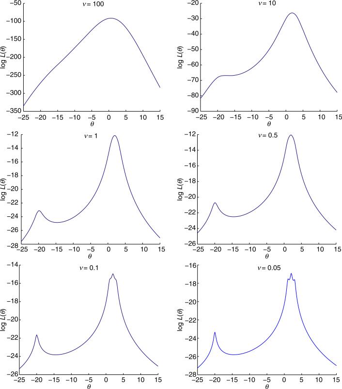
We now illustrate annealing by a classical textbook example for the univariate t (Arslan et al., 1993; McLachlan & Krishnan, 2008). The data consist of the four observations −20, 1, 2 and 3. The scale Ω = 1 and degrees of freedom α = 0.05 are fixed. The bottom right panel of Fig. 1 shows that the log-likelihood function has modes at −19.9932, 1.0862, 1.9975 and 2.9056 for the given scale and degrees of freedom. The global mode $\widehat{\mu }=1.9975$ reflects the successful downweighting of the outlier −20 by the t model. The remaining panels of Fig. 1 illustrate the warping of the log-likelihood surface for different values of ν.

Fig. 1.

The log-likelihood ln L(μ) for various degrees of freedom ν with Ω = 1.

Table 1 records the progress of the fast EM algorithm and the aEM1 algorithm starting from the bad guess μ⁰ = −25. For the aEM1 algorithm, we take r = 0.5 and s = 1 and start the tuning parameter at ν⁰ = 100. The EM algorithm gets quickly sucked into the inferior mode −19.9932, whereas the aEM1 algorithm rapidly converges to the global mode. Doubtful readers may object that the poor performance of EM is an artefact of a bad initial value, but starting from the sample mean −3.5 leads to the inferior mode 1.0862. Starting from the sample median 1.5 does lead to the dominant mode in this example. Table 1 does not cover the performance of algorithms aEM2 and aEM3. Algorithm aEM2 collapses to the ordinary EM algorithm in fixing Ω, and algorithms aEM3 and aEM1 perform almost identically.

Table 1.

EM and aEM1 iterates starting from μ⁰ = –25 when α = 0.05 and Ω = 1

Iter	EM		aEM1
n	μ n	ln L(μn)	μ n	ln L(μn)	ν n
1	–25.0000	–27.2613	–25.0000	–27.2613	100.0000
2	–17.9437	–25.3781	–13.1518	–25.7683	50.0250
3	–19.3111	–24.4855	–8.7916	–25.2122	25.0375
4	–19.9239	–23.3984	–3.2796	–23.3531	12.5438
5	–19.9923	–23.3513	0.8913	–17.8380	6.2969
6	–19.9932	–23.3513	1.7023	–17.3523	3.1734
7	–19.9932	–23.3513	1.8561	–17.0700	1.6117
8	–19.9932	–23.3513	1.9060	–16.9867	0.8309
9	–19.9932	–23.3513	1.9310	–16.9539	0.4404
10	–19.9932	–23.3513	1.9509	–16.9340	0.2452
11	–19.9932	–23.3513	1.9695	–16.9213	0.1476
12	–19.9932	–23.3513	1.9837	–16.9156	0.0988
13	–19.9932	–23.3513	1.9916	–16.9141	0.0744
14	–19.9932	–23.3513	1.9951	–16.9139	0.0622
15	–19.9932	–23.3513	1.9965	–16.9138	0.0561
16	–19.9932	–23.3513	1.9971	–16.9138	0.0531
17	–19.9932	–23.3513	1.9973	–16.9138	0.0515
18	–19.9932	–23.3513	1.9974	–16.9138	0.0508
19	–19.9932	–23.3513	1.9974	–16.9138	0.0504
20	–19.9932	–23.3513	1.9975	–16.9138	0.0502
21	–19.9932	–23.3513	1.9975	–16.9138	0.0501
22	–19.9932	–23.3513	1.9975	–16.9138	0.0500

Multimodality is not limited to extremely small values of α. For the three data points {0, 5, 9}, the likelihood of the Cauchy distribution (α = 1 and Ω = 1) has three modes (example 1.9 of Robert & Casella, 2004). The aEM algorithms easily leap across either inferior mode and converge to the middle global mode. For the sake of brevity we omit details.

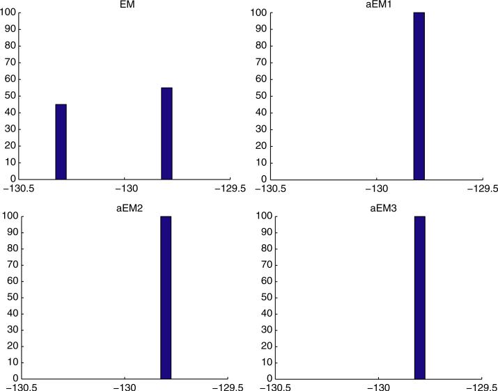
In analysing the random data from a bivariate t distribution displayed in Table 2, we assume α = 0.1 is known and both μ and Ω are unknown. The histograms of the final log-likelihoods found by the fast EM algorithm and the aEM algorithms from the same 100 random starting points are shown in Fig. 2. A total of 45 runs of the EM algorithm converge to the inferior mode at −130.28, whereas all runs of the aEM algorithms converge to the global mode −129.8. Despite this encouraging performance, annealing is not foolproof. There exist more extreme examples where the aEM algorithms consistently converge to an inferior mode close to the centre of the sample points. This problem merits further research.

Table 2.

Twenty-five data points generated from a bivariate t distribution

–0.7252	0.5627	0.2584	1.5761	–0.0830	0.8445
–0.8550	–0.1086	–0.3399	0.6621	–3.8701	–5.3761
0.1062	–0.9193	0.7471	1.4070	0.3264	0.6519
0.2629	–0.7877	–0.5796	–1.2631	–10.044	–5.6143
–0.7699	–0.2417	213.62	143.72	3. 2176	–0.8608
3.0981	1.3417	–0.2335	–0.3554	1.8424	–0.5556
2.2407	2.4764	0.0540	–0.5216	–2.1804	–1.6183
–0.0518	0.7885	1.1241	0.9627
0.6448	1.4672	0.0397	–0.4924

Fig. 2.

Histograms of the converged log-likelihoods found by the EM (top left panel) and aEM algorithms from 100 random starting points for the data in Table 2. For aEM1, ν⁰ = 100, r = 0.5 and s = 10. For aEM2 and aEM3, ν⁰ = 0.001, r = 0.5 and s = 10.

4. Finite mixture models

In admixture models, the likelihood of m independent observations x₁,..., x_m takes the form

$$L(\pi ,\theta )=\prod _{i=1}^m\sum _{j=1}^d{\pi }_j{f}_j(x_i\mid {\theta }_j),$$

where π = (π₁,..., π_d) is the vector of admixture parameters and f_j(x|θ_j) is the density of the jth admixture component. This model is widely used in soft clustering; see Bouguila (2008) for recent applications to clustering of images, handwritten digits and online documents. As we mentioned previously, Ueda & Nakano (1998) redesign the standard EM algorithm to incorporate deterministic annealing. The MM principle provides new insight into the derivation and application of annealing in this setting. In our opinion, admixture annealing deserves more attention from the statistics community. To illustrate our point, we discuss applications to latent class models popular in the social sciences.

In the admixture model we can flatten the likelihood surface in two different ways. These give rise to the objective functions

$$\begin{array}{cc}\hfill L_1(\pi ,\theta ,v)& =\prod _{i=1}^m\sum _{j=1}^d{\left[{\pi }_j{f}_j(x_i\mid {\theta }_j)\right]}^v,\hfill \\ \hfill L_2(\pi ,\theta ,v)& =\prod _{i=1}^m\sum _{j=1}^d{\pi }_j{\left[f_j(x_i\mid {\theta }_j)\right]}^v,\hfill \end{array}$$

appropriate for annealing. Here ν varies over the interval [0, 1]. The choice ν = 0 produces a completely flat surface, and the choice ν = 1 recovers the original surface. This suggests that we gradually increase the tuning parameter ν from a small value such as 0.05 all the way to 1. At each level of ν we execute s steps of the EM algorithm or its MM substitute.

In the admixture setting, the MM principle exploits the concavity of the function ln(t). Applying Jensen's inequality to ln L₁(π, θ, ν) yields the minorization

$$\sum _{i=1}^m\ln \left\{\sum _{j=1}^d{\left[{\pi }_j{f}_j(x_i\mid {\theta }_j)\right]}^v\right\}\ge \sum _{i=1}^m\sum _{j=1}^d{w}_{ij}^n\ln \left\{\frac{{\left[{\pi }_j{f}_j(x_i\mid {\theta }_j)\right]}^v}{w_{ij}^n}\right\}=v\sum _{i=1}^m\sum _{j=1}^d{w}_{ij}^n[\ln {\pi }_j+\ln f_j(x_i\mid {\theta }_j)]+c^n,$$

where the weights are

$$w_{ij}^n=\frac{{\left[{\pi }_j^n{f}_j(x_i\mid {\theta }_j^n)\right]}^v}{\sum _{k=1}^d{\left[{\pi }_k^n{f}_k(x_i\mid {\theta }_k^n)\right]}^v}$$ (4)

and cⁿ is an irrelevant constant. Minorization separates the π parameters from the θ_j parameters and allows one to solve for the updates

$${\pi }_j^{n+1}=\frac{\sum _{i=1}^m{w}_{ij}^n}{\sum _{i=1}^m\sum _{k=1}^d{w}_{ik}^n}.$$

The usual manoeuvres yield the MM updates for the θ_k parameters in standard models. These updates are identical to the standard EM updates except for the differences in weights.

Minorization of ln L₂(π, θ, ν) follows in exactly the same manner except that the weights become

$$w_{ij}^n=\frac{{\pi }_j^n{f}_j{(x_i\mid {\theta }_j^n)}^v}{\sum _{k=1}^d{\pi }_k^n{f}_k{(x_i\mid {\theta }_k^n)}^v}.$$ (5)

One of the virtues of this MM derivation is that it eliminates the need for normalization of probability densities.

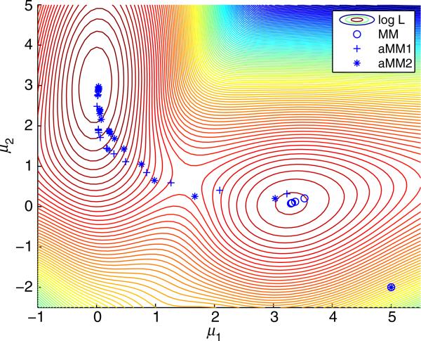
To compare the MM and aMM algorithms, consider a Gaussian mixture model with two components, fixed proportions π₁ = 0.7 and π₂ = 0.3 and fixed standard deviations σ₁ = 0.5 and σ₂ = 1. The means (μ₁, μ₂) are the parameters to be estimated. Figure 3 shows the progress of the MM and aMM algorithms based on 500 random Gaussian deviates with μ₁ = 0 and μ₂ = 3. From the poor starting point (μ₁, μ₂) = (5, −2), the MM algorithm leads to the inferior local mode (3.2889, 0.0524) whereas the two aMM algorithms successfully converge to the global mode (0.0282, 3.0038). Here we start with ν⁰ = 0.1 and after each s = 5 iterations multiply ν by r = 2 until it reaches 1, i.e., every 5 iterations we replace the current value νⁿ of ν by νⁿ⁺¹ = min{2νⁿ,1}. The evidence here suggests that the two forms of aMM perform about equally well.

Fig. 3.

Progress of MM and two aMM algorithms in the log-likelihood landscape of a Gaussian mixture model.

Latent class analysis (LCA) is a discrete analogue of cluster analysis. It seeks to define clusters and assign subjects to them. For instance, a political party might cluster voters by answers to questions on a survey. The data could reveal conservative and liberal clusters or wealthy and poor clusters. The hidden nature of the latent classes suggest application of the EM algorithm. Unfortunately, maximum likelihood estimation with LCA is again beset by the problem of local modes.

For purposes of illustration, consider the simple latent class model of Goodman (1974) in which there are d latent classes and each subject is tested on b Bernoulli items. Conditional on the subject's latent class, the b tests are independent. The subject's binary response vector y = (y₁,..., y_b) therefore has probability

$$\mathrm{Pr}(Y=y)=\sum _{j=1}^d{\pi }_j\prod _{k=1}^b{\theta }_{jk}^{y_k}{(1-{\theta }_{jk})}^{1-y_k},$$

where the π_j are admixture proportions, and the θ_jk are success probabilities. If c_y counts the number of subjects with response vector y, then the log-likelihood is

$$\ln L(p,\pi )=\sum _y{c}_y\ln \left[\sum _{j=1}^d{\pi }_j\prod _{k=1}^b{\theta }_{jk}^{y_k}{(1-{\theta }_{jk})}^{1-y_k}\right].$$

Introducing the weights

$$w_{yj}^n=\frac{{\pi }_j^n\prod _{k=1}^b{\left({\theta }_{jk}^n\right)}^{y_k}{(1-{\theta }_{jk}^n)}^{1-y_k}}{\sum _{l=1}^d{\pi }_l^n\prod _{k=1}^b{\left({\theta }_{lk}^n\right)}^{y_k}{(1-{\theta }_{lk}^n)}^{1-y_k}},$$

one can easily derive the MM updates

$${\pi }_j^{n+1}=\frac{\sum _y{c}_y{w}_{yj}^n}{\sum _{l=1}^d\sum _y{c}_y{w}_{yl}^n},{\theta }_{jk}^{n+1}=\frac{\sum _y{c}_y{y}_k{w}_{yj}^n}{\sum _y{c}_y{w}_{yj}^n}.$$

For annealing, we can define the revised weights (4) and (5) using the densities

$$f_j(y\mid {\theta }_j)=\prod _{k=1}^b{\theta }_{jk}^{y_k}{(1-{\theta }_{jk})}^{1-y_k}.$$

The MM updates remain the same except for substitution of the revised weights for the ordinary weights.

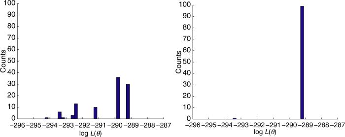
For a numerical example, we now turn to a classical data set on pathology rating (section 13.1.2 in Agresti, 2002). Seven pathologists classified each of 118 slides for the presence or absence of carcinoma of the uterine cervix. Assuming d = 4 latent classes, we ran both MM and aMM (version 1) starting from the same 100 random starting points; we declared convergence when the relative change of the log-likelihood was less than 10⁻⁹. Figure 4 displays the histograms of the converged log-likelihoods for the two algorithms. In 99 out of 100 runs, the aMM converges to what appears to be the global mode. Fewer than one-third of the MM runs converge to this mode. The maximum likelihood estimates of the π_j and θ_jk at the global mode are listed in Table 3. These results suggest that: (i) the first latent class captures those cases with good agreement that carcinoma exists; (ii) the second latent class captures those cases with good agreement that carcinoma does not exist; (iii) the third latent class captures cases with strong disagreement, with pathologists A, B, C, D and E suggesting carcinoma and pathologists D and F suggesting otherwise; and (iv) the fourth latent class captures the residual of problematic cases. Convergence to a local mode can lead to quite different interpretations. The parameter estimates in Table 4 for the inferior mode with log-likelihood −293.3200 presents a very different picture.

Fig. 4.

Final log-likelihoods found for the pathology data set by MM (left) and aMM (right) using 100 random starting points. The annealing parameters are ν = 0.05, s = 10 and r = 19/20.

Table 3.

Maximum likelihood estimates for the pathology data. The log-likelihood at this mode is –289.2859

Latent class	$\text{Pathologist}{\widehat{\theta }}_{jk}$
${\widehat{\pi }}_j$	A	B	C	D	E	F	G
0.3430	1.0000	1.0000	0.8439	0.7579	1.0000	0.6177	1.0000
0.3751	0.0578	0.1415	0	0	0.0557	0	0
0.0938	1.0000	0.9096	0.9802	0.0000	1.0000	0.0000	1.0000
0.1881	0.5363	1.0000	0	0.0597	0.7657	0	0.6515

Table 4.

Estimates at a local mode for the pathology data. The corresponding log-likelihood is –293.3200

Latent class	$\text{Pathologist}{\widehat{\theta }}_{jk}$
${\widehat{\pi }}_j$	A	B	C	D	E	F	G
0.4441	1.0000	0.9809	0.8588	0.5867	1.0000	0.4771	1.0000
0.3544	0.0000	0.1390	0	0	0.0593	0	0
0.0281	1.0000	0.3958	0	0	0	0	0
0.1735	0.5025	1.0000	0	0.0615	0.7872	0	0.6642

5. Factor analysis

Factor analysis models the covariation among the components of a random vector Y with p components as the sum

$$Y=\mu +FX+U,$$

where μ is a constant vector with p components, F is a p × q constant matrix, X is random vector with q components and U is a random vector with p components. These quantities are termed the mean vector, the factor loading matrix, the factor score and the noise, respectively. Ordinarily, q is much smaller than p. In addition, the standard model postulates that X and U are independent Gaussian random vectors with means and variances

$$\begin{array}{cc}\hfill E\left(X\right)& =0,\text{var}\left(X\right)=I\hfill \\ \hfill E\left(U\right)& =0,\text{var}\left(U\right)=D,\hfill \end{array}$$

where D is diagonal with jth diagonal entry d_j. Given a random sample y₁,..., y_m from the model distribution, the object is to estimate μ, F and D. As the log-likelihood is

$$\ln L=-\frac{m}{2}\ln \text{det}(F{F}^t+D)-\frac{1}{2}\sum _{k=1}^m{(y_k-\mu )}^t{(F{F}^t+D)}^{-1}(y_k-\mu ),$$

it is clear that the maximum likelihood estimate of μ equals the sample mean. Therefore, we eliminate μ from the model and assume that the data are centred at 0.

Estimation of F and D is afflicted by identifiability issues and the existence of multiple modes. In practice, the latter are more troublesome than the former. We attack the multiple mode problem by flattening the log-likelihood surface. This can be achieved by maximizing

$$\ln L+\frac{v}{2}\ln \text{det}D=\ln L+\frac{v}{2}\sum _{j=1}^p\ln d_j$$

for ν∈[0, m). In effect, this inflates the noise component of the model. We progressively adjust ν from near m to 0.

The EM algorithm is the workhorse of factor analysis, so it is natural to modify it to take into account the added noise. The complete data in the EM algorithm for estimating F and D are the random vectors (Y_k, X_k) for each case k. The noise term of the objective function has no effect on the derivation of the EM surrogate, which up to an irrelevant constant equals

$$Q(F,D\mid F^n,D^n)=-\frac{m}{2}\sum _{j=1}^p\ln d_j-\frac{1}{2}tr\left[D^{-1}(F\Lambda F^t-F\Gamma -{\Gamma }^t{F}^t+\Omega )\right].$$

Here, the intermediate vectors and matrices are

$$\Lambda =\sum _{k=1}^m[A_k+v_k{v}_k^t],\Gamma =\sum _{k=1}^m{v}_k{y}_k^t,\Omega =\sum _{k=1}^m{y}_k{y}_k^t,$$

with

$$v_k=F^t{(F{F}^t+D)}^{-1}{y}_k,A_k=I-F^t{(F{F}^t+D)}^{-1}F.$$

In defining v_k and A_k, the matrices F and D are evaluated at their current estimates Fⁿ and Dⁿ. The full derivation of the surrogate function appears in section 7.5 of Lange (2004).

The MM principle suggests that we maximize the surrogate $Q+\frac{v}{2}\ln \text{det}D$ rather than the objective function $\ln L+\frac{v}{2}\ln \text{det}D$. If one follows the mathematical steps outlined in Lange (2004), then it is straightforward to verify the MM updates

$$\begin{array}{cc}\hfill F^{n+1}& ={\Gamma }^t{\Lambda }^{-1},\hfill \\ \hfill d_i^{n+1}& =\frac{1}{m-v}{[F^{n+1}\Lambda {\left(F^{n+1}\right)}^t-F^{n+1}\Gamma -{\Gamma }^t{\left(F^{n+1}\right)}^t+\Omega ]}_{ii}.\hfill \end{array}$$

It is obvious from the form of the update for the noise variance d_i that the amendment to the likelihood pushes the estimate of d_i higher.

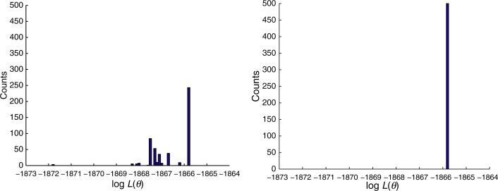
For a numerical example, we now consider the classic data of Maxwell (1961). There are p = 10 variables and m = 148 subjects. The variables summarize various psychiatric tests on 148 children: (i) verbal ability, (ii) spatial ability, (iii) reasoning, (iv) numerical ability, (v) verbal fluency, (vi) neuroticism questionnaire, (vii) ways to be different, (viii) worries and anxieties, (ix) interests, and (x) annoyances. Table 5 lists the correlations between the 10 variables. Maxwell (1961) concludes that three factors adequately capture the variation in the data. To illustrate the problem of multiple modes, we assume q = 5 factors, giving a total of p(q+1) = 60 parameters. We ran both EM and aEM on the same 500 random starting points and stopped each run when the relative change of the log-likelihood was less than 10⁻⁹. Figure 5 shows the histograms of the converged log-likelihoods found by the two algorithms. In all 500 runs, the aEM algorithm converges to the same mode. Fewer than half of the EM runs converge to this apparently global mode. Our discovery of several inferior modes confirms previous findings (Duan & Simonato, 1993). Table 6 lists the estimates of the noise variances d_i at the global and two local modes. In this example, we start with ν = m−1 = 148 and halve it every five iterations.

Table 5.

Correlations of 10 variables in the Maxwell data

Test	2	3	4	5	6	7	8	9	10
1	0.533	0.598	0.532	0.550	–0.225	–0.270	–0.093	–0.214	–0.130
2		0.419	0.282	0.276	0.017	–0.136	–0.010	–0.216	–0.162
3			0.532	0.558	–0.067	–0.226	0.024	–0.159	–0.008
4				0.518	–0.118	–0.154	–0.096	–0.096	0.023
5					–0.126	–0.148	–0.049	–0.025	0.000
6						0.373	0.519	0.218	0.334
7							0.483	0.400	0.435
8								0.276	0.390
9									0.332

Fig. 5.

Converged log-likelihoods found by EM (left) and aEM (right) from 500 random starting points. For aEM, ν⁰ = 147, r = 1/2 and s = 5.

Table 6.

Estimates of d_i at different three modes

	Mode
ln L	–1865.8	–1867.5	–1871.8
d̂ 1	0.3095	0.0090	0.3122
d̂ 2	0.0275	0.5916	0.4993
d̂ 3	0.3536	0.0106	0.4236
d̂ 4	0.4956	0.1921	0.0212
d̂ 5	0.4582	0.5448	0.3605
d̂ 6	0.5274	0.4722	0.5548
d̂ 7	0.4187	0.4892	0.5389
d̂ 8	0.0206	0.4233	0.3851
d̂ 9	0.6840	0.6539	0.6958
d̂ 10	0.5859	0.5903	0.0201

6. Multidimensional scaling

Multidimensional scaling attempts to represent q objects as faithfully as possible in p-dimensional space given a non-negative weight w_ij and a non-negative dissimilarity measure y_ij for each pair of objects i and j. If ${\theta }_i\in {\mathbb{R}}^p$ is the position of object i, then the p × q parameter matrix θ with ith column θ_i is estimated by minimizing the stress

$$\begin{array}{cc}\hfill {\sigma }^2\left(\theta \right)& =\sum _{1\le i<j\le q}{w}_{ij}{(y_{ij}-\Vert {\theta }_i-{\theta }_j\Vert )}^2\hfill \\ \hfill & =\sum _{1\le i<j\le q}{w}_{ij}{y}_{ij}^2-2\sum _{1\le i<j\le q}{w}_{ij}{y}_{ij}\Vert {\theta }_i-{\theta }_j\Vert +\sum _{1\le i<j\le q}{w}_{ij}{\Vert {\theta }_i-{\theta }_j\Vert }^2,\hfill \end{array}$$ (6)

where $\Vert {\theta }_i-{\theta }_j\Vert$ is the Euclidean distance between θ_i and θ_j. The stress function (6) is invariant under translations, rotations and reflections of ${\mathbb{R}}^p$. To avoid translational and rotational ambiguities, we take θ₁ to be the origin and the first p−1 coordinates of θ₂ to be 0. Switching the sign of θ_2p leaves the stress function invariant. Hence, convergence to one member of a pair of reflected minima immediately determines the other member.

The stress function tends to have multiple local minima in low dimensions (Groenen & Heiser, 1996). As the number of dimensions increases, most of the inferior modes disappear. In support of this contention, one can mathematically demonstrate that the stress has a unique minimum when p = q−1 (de Leeuw, 1993; Groenen & Heiser, 1996). In practice, uniqueness can set in well before p reaches q−1. In dimension crunching, we start optimizing the stress in some space ${\mathbb{R}}^m$ with m>p. The last m−p components of each θ_i are gradually subjected to stiffer and stiffer penalties. In the limit as the penalty tuning parameter ν tends to ∞, we recover the minimum of the stress in ${\mathbb{R}}^p$. Before we go into the details of how crunching is achieved, it is helpful to review the derivation of the MM stress updates given in Lange et al. (2000).

Because we want to minimize the stress, we first majorize it. In doing so, it is helpful to separate its parameters as well. The middle term in the stress (6) is majorized by the Cauchy–Schwartz inequality

$$-\Vert {\theta }_i-{\theta }_j\Vert \le -\frac{{({\theta }_i-{\theta }_j)}^t({\theta }_i^n-{\theta }_j^n)}{\Vert {\theta }_i^n-{\theta }_j^n\Vert }.$$

To separate the variables in the summands of the third term of the stress, we invoke the convexity of the Euclidean norm $\Vert \cdot \Vert$ and the square function x². These manoeuvres yield

$${\Vert {\theta }_i-{\theta }_j\Vert }^2={\Vert \frac{1}{2}\left[2{\theta }_i-({\theta }_i^n+{\theta }_j^n)\right]-\frac{1}{2}\left[2{\theta }_j-({\theta }_j^n+{\theta }_j^n)\right]\Vert }^2\le 2{\Vert {\theta }_i-\frac{1}{2}({\theta }_i^n+{\theta }_j^n)\Vert }^2+2{\Vert {\theta }_j-\frac{1}{2}({\theta }_i^n+{\theta }_j^n)\Vert }^2.$$

Assuming that w_ij = w_ji and y_ij = y_ji, the surrogate function therefore becomes

$$2\sum _{i<j}{w}_{ij}\left[{\Vert {\theta }_i-\frac{1}{2}({\theta }_i^n+{\theta }_j^n)\Vert }^2-\frac{y_{ij}{\theta }_i^t({\theta }_i^n-{\theta }_j^n)}{\Vert {\theta }_i^n-{\theta }_j^n\Vert }\right]+2\sum _{i<j}{w}_{ij}\left[{\Vert {\theta }_j-\frac{1}{2}({\theta }_i^n+{\theta }_j^n)\Vert }^2+\frac{y_{ij}{\theta }_j^t({\theta }_i^n-{\theta }_j^n)}{\Vert {\theta }_i^n-{\theta }_j^n\Vert }\right]=2\sum _{i=1}^q\sum _{j\ne i}\left[w_{ij}{\Vert {\theta }_i-\frac{1}{2}({\theta }_i^n+{\theta }_j^n)\Vert }^2-\frac{w_{ij}{y}_{ij}{\theta }_i^t({\theta }_i^n-{\theta }_j^n)}{\Vert {\theta }_i^n-{\theta }_j^n\Vert }\right]$$

up to an irrelevant constant.

Setting the gradient of the surrogate equal to 0 vector gives the updates

$${\theta }_{ik}^{n+1}=\frac{\sum _{j\ne 1}\left[\frac{w_{ij}{y}_{ij}({\theta }_{ik}^n-{\theta }_{jk}^n)}{\Vert {\theta }_i^n-{\theta }_j^n\Vert }+w_{ij}({\theta }_{ik}^n+{\theta }_{jk}^n)\right]}{2\sum _{j\ne i}{w}_{ij}}$$

for all movable parameters θ_ik. To perform annealing, we add the penalty $v{\sum }_{i=1}^q{\sum }_{j=p+1}^m{\theta }_{ij}^2$ to the stress function and progressively increase ν from nearly 0 to ∞. This action shrinks the last m−p components of each θ_i to 0. It is straightforward to check that the updates for the penalized stress are

$$\begin{array}{cc}\hfill {\theta }_{ik}^{n+1}& =\frac{\sum _{j\ne i}\left[\frac{w_{ij}{y}_{ij}({\theta }_{ik}^n-{\theta }_{jk}^n)}{\Vert {\theta }_i^n-{\theta }_j^n\Vert }+w_{ij}({\theta }_{ik}^n+{\theta }_{jk}^n)\right]}{2\sum _{j\ne i}{w}_{ij}},1\le k\le p\hfill \\ \hfill {\theta }_{ik}^{n+1}& =\frac{\sum _{j\ne i}\left[\frac{w_{ij}{y}_{ij}({\theta }_{ik}^n-{\theta }_{jk}^n)}{\Vert {\theta }_i^n-{\theta }_j^n\Vert }+w_{ij}({\theta }_{ik}^n+{\theta }_{jk}^n)\right]}{2\left(\sum _{j\ne i}{w}_{ij}+v\right)},p+1\le k\le m.\hfill \end{array}$$

Taking m = q − 1 is computationally expensive if q is large. In this situation, we typically choose m much smaller than q but still considerably larger than p.

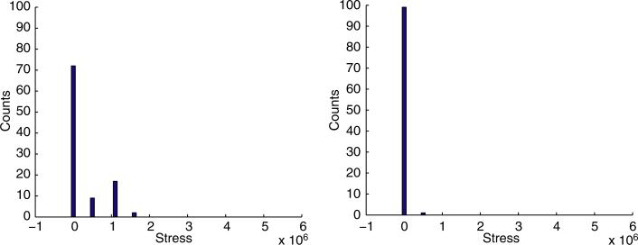
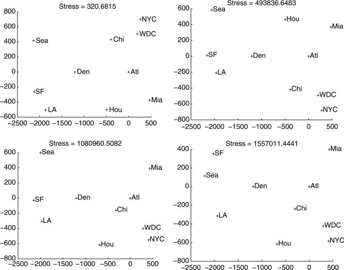
For the US city distance data summarized in Table 7, we ran both the MM and aMM algorithms for multidimensional scaling with w_ij = 1 and p = 2 from 100 random starting points. For aMM we set m = 9, started with ν = 0.001 and multiplied ν by 1.1 every 10 iterations. The histogram of final converged stress values are displayed in Fig. 6. It is gratifying that 97 runs of aMM converge to the global minimum 321.68 whereas only 59 runs of MM do. Figure 7 shows the city configurations from multidimensional scaling at different local minima.

Table 7.

Distances between q = 10 US cities

	Chi	Den	Hou	LA	Mia	NYC	SF	Sea	WDC
Atl	587	1212	701	1936	604	748	2139	2182	543
Chi		920	940	1745	1188	713	1858	1737	597
Den			879	831	1726	1631	949	1021	1494
Hou				1374	968	1420	1645	1891	1220
LA					2339	2451	347	959	2300
Mia						1092	2594	2734	923
NYC							2571	2408	205
SF								678	2442
Sea									2329

Chicago (Chi), Denver (Den), Houston (Hou), Los Angeles (LA), Miami (Mia), New York (NYC), San Francisco (SF), Seattle (Sea), Washington (WDC)

Fig. 6.

Final stress values found by MM (left) and aMM (right) from 100 random starting points. The annealing parameters are ν⁰ = 0.001, r = 1.1 and s = 10.

Fig. 7.

Multidimensional scaling maps of the 10 cities at various local modes of the stress function.

7. A one-way random effects model

Our last example is novel in three respects. It is Bayesian, it yields readily to maximum a posteriori estimation by block relaxation, and its transition from unimodality to bimodality is fairly well understood mathematically. In the one-way random-effects model described by Liu & Hodges (2003), the data are modelled as y_ij|θ_i, σ² ~ N(θ_i, σ²), j = 1,..., r_i, where the θ_i are unobserved random effects distributed as θ_i|μ, τ² ~ N(μ, τ²), i = 1,..., s. The hyperparameters μ, σ² and τ² are unknown. In a Bayesian framework it is convenient to assume conjugate priors for them of the form μ ~ N(ν, η²), σ² ~ IG(α, β) and τ² IG(γ, δ), where IG denotes the inverse Gamma distribution parameterized so that E(σ²) ~ = β/(α − 1) and E(τ²) = δ/(γ 1) for α and γ exceeding 1.

The joint probability density of the data and parameters ({y_ij}, {θ_i}, μ, σ², τ²) is

$$\prod _{i,j}{\left(2\pi {\sigma }^2\right)}^{-1∕2}{\mathrm{e}}^{-\left({(y_{ij}-{\theta }_i)}^2\right)∕\left(2{\sigma }^2\right)}\prod _i{\left(2\pi {\tau }^2\right)}^{-1∕2}{\mathrm{e}}^{-\left({({\theta }_i-\mu )}^2\right)∕\left(2{\tau }^2\right)}{\left(2\pi {\eta }^2\right)}^{-1∕2}{\mathrm{e}}^{-\left({(\mu -v)}^2\right)∕\left(2{\eta }^2\right)}\times \frac{{\beta }^{\alpha }}{\Gamma \left(\alpha \right)}{\left({\sigma }^2\right)}^{-\alpha -1}{\mathrm{e}}^{-\beta ∕{\sigma }^2}\frac{{\delta }^{\gamma }}{\Gamma \left(\gamma \right)}{\left({\tau }^2\right)}^{-\gamma -1}{\mathrm{e}}^{-\delta ∕{\tau }^2}.$$

This translates into the log-posterior function

$$P(\left\{{\theta }_i\right\},\mu ,{\sigma }^2,{\tau }^2\mid \left\{y_{ij}\right\})=-\frac{\sum _i{r}_i+2\alpha +2}{2}\text{log}\left({\sigma }^2\right)-\frac{2\beta +\sum _{i,j}{(y_{ij}-{\theta }_i)}^2}{2{\sigma }^2}-\frac{s+2\gamma +2}{2}\text{log}\left({\tau }^2\right)-\frac{2\delta +\sum _i{({\theta }_i-\mu )}^2}{2{\tau }^2}-\frac{{(\mu -v)}^2}{2{\eta }^2}+c,$$

where c is an irrelevant constant. Maximum a posteriori estimation can be an end in itself or a prelude to a full Bayesian analysis by Markov chain Monte Carlo or Laplace approximation (Rue et al., 2009).

The direct attempt to maximize the log-posterior is almost immediately thwarted. It is much easier to implement block relaxation, which maximizes the objective function over successive parameter subsets. Like the EM or MM algorithms, block relaxation enjoys the ascent property. With the superscripts k and k+1 denoting iteration numbers, block relaxation operates via the updates

$$\begin{array}{cc}\hfill & {\theta }_i^{k+1}=\frac{\frac{\sum _{j=1}^{r_i}{y}_{ij}}{{\left({\sigma }^2\right)}^k}+\frac{{\mu }^k}{{\left({\tau }^2\right)}^k}}{\frac{r_i}{{\left({\sigma }^2\right)}^k}+\frac{1}{{\left({\tau }^2\right)}^k}},i=1,\dots ,s,\hfill \\ \hfill & {\mu }^{k+1}=\frac{\frac{\sum _{i=1}^s{\theta }_i^{k+1}}{{\left({\tau }^2\right)}^{k+1}}+\frac{v}{{\eta }^2}}{\frac{s}{{\left({\tau }^2\right)}^{k+1}}+\frac{1}{{\eta }^2}},\hfill \\ \hfill & {\left({\sigma }^2\right)}^{k+1}=\frac{2\beta +\sum _{i,j}{(y_{ij}-{\theta }_i^{k+1})}^2}{\sum _i{r}_i+2\alpha +2},\hfill \\ \hfill & {\left({\tau }^2\right)}^{k+1}=\frac{2\delta +\sum _{i=1}^s{({\theta }_i^{k+1}-{\mu }^{k+1})}^2}{s+2\gamma +2}.-\hfill \end{array}$$

In the case of a balanced design where the sample sizes r_i are equal, Liu & Hodges (2003) systematically study the modality of the log-posterior and determine how it depends on the parameters α, β, γ, δ and the data {y_ij}. They assume a flat prior on μ, achieved by taking ν = 0 and η² = ∞. Under a flat prior, the joint posterior distribution is proper, and our block relaxation algorithm remains valid. It is noteworthy that their theorem 1 implies that the joint posterior has at most two modes. Furthermore, their theorem 3 implies that in the presence of bimodality, increasing α or δ with all other parameters fixed extinguishes one of the modes, whereas increasing β or γ with all other parameters fixed extinguishes the other mode. This insight immediately suggests a two-run annealing procedure that is almost guaranteed to identify the global maximum. In the first run, we replace α (or δ) in block relaxation by a large tuning parameter α^k (or δ^k) and gradually sent it to its limiting value. In the second run, we replace β (or γ) in block relaxation by a large tuning parameter β^k (or γ^k) and gradually sent it to its limiting value. If the two final modes agree, then the log-posterior is unimodal. If they disagree, then one of them is bound to be the global mode.

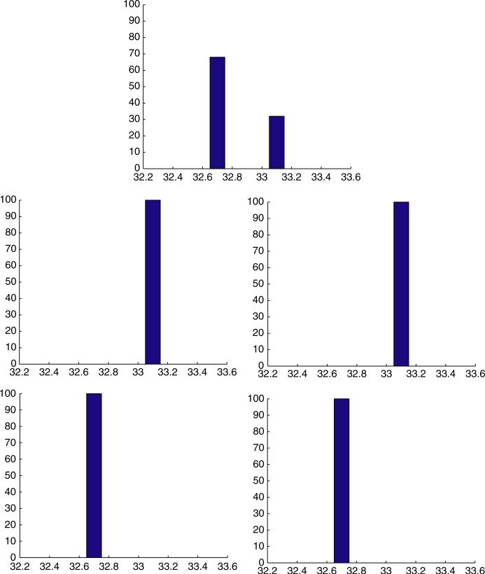
As an example, we tested the peak discharge data analysed by Liu & Hodges (2003). With the settings α = 8, β = 1, γ = 10 and δ = 0.1, the log-posterior has two modes. We tried ordinary block relaxation and four versions of deterministic annealing from 100 randomly generated points. As Fig. 8 shows, every run of deterministic annealing reliably converges to its targeted mode. It would appear that the two-run tactic is highly successful.

Fig. 8.

Histograms of converged posterior log-likelihoods (up to an additive constant) under different annealing schemes from 100 random starting points. Here, s = 1 and r 0.5. Top: no annealing; middle left: b⁰ = 10³; middle right: α⁰ = 10³; bottom left: a⁰ = 10³; bottom right: β⁰ = 10³.

8. Discussion

The existence of multiple modes is one of the nagging problems of computational statistics. No one knows how often statistical inference is fatally flawed because a standard optimization algorithm converges to an inferior mode. Although the traditional remedies can eliminate the problem, they enjoy no guarantees. Bayesian inference is also not a refuge. Markov Chain Monte Carlo (MCMC) sampling often gets stuck in the vicinity of an inferior posterior mode, and it may be hard to detect departures from adequate random sampling. For these reasons, any technique for finding the dominant mode of a log-likelihood or a log-posterior function is welcome.

It is probably too much to hope for a panacea. Continuous optimization by simulated annealing comes close, but it imposes an enormous computational burden. The recent marriage of computational statistics and algebraic geometry has considerable promise (Pachter & Sturmfels, 2005). The new field, algebraic statistics, attempts to locate all of the modes of a likelihood function. This is probably too ambitious, and current progress is limited to likelihoods composed of simple polynomials and rational functions.

The EM annealing algorithm of Ueda & Nakano (1998) deserves wider use. In our opinion, the MM principle clarifies its derivation and frees it from the restriction to probability densities. In multidimensional scaling, the tunnelling method of Groenen & Heiser (1996) is a competitor to dimension crunching. It would be worthwhile to undertake a systematic comparison. Several, but not all, of the annealing techniques used for the multivariate t distribution extend to other elliptically symmetric families of densities such as the slash family (Lange & Sinsheimer, 1993). We will let readers explore the relevant algorithms at their leisure.

We would be remiss if we did not confess to experimenting with the annealing parameters ν⁰, r and s to give good performance. We have not been terribly systematic because a broad range of values works well in many problems. Again, this is an area worthy of further investigation. Rigid guidelines are less important than rules of thumb.

In closing, let us emphasize that our purpose has been to introduce basic strategies rather than detailed tactics. Wider application of annealing will require additional devices for flattening function surfaces and moving towards the global mode. Although the MM algorithm is one among many choices, its simplicity and ascent (or descent) property are very attractive. MM algorithms tend to home in quickly on the basis of attraction of the dominant mode. Once an MM algorithm reaches this region, its rate of progress can slow dramatically. Thus, many annealing algorithms have to be accelerated to be fully effective. The challenge for the statistics community is to tackle a wider range of statistical models with multiple modes. This will have to be done piecemeal to sharpen intuition before we can hope to make a general assault on this vexing general problem.

Appendix. Pseudocode For EM algorithms

Algorithm 1.

EM.

Initialize: μ0, Ω0

repeat

$w_i^n\leftarrow \frac{\alpha +p}{\alpha +d_i^n},v^n\leftarrow {\sum }_{i=1}^m{w}_i^n$

${\mu }^{n+1}\leftarrow \frac{1}{v^n}{\sum }_{i=1}^m{w}_i^n{x}_i$

${\Omega }^{n+1}\leftarrow \frac{1}{v^n}{\sum }_{i=1}^m{w}_i^n(x_i-{\mu }^{n+1}){(x_i-{\mu }^{n+1})}^t$

Until convergence occurs

Algorithm 2.

aEM1 (inflating degree of freedom).

Initialize: μ0, Ω0, ν0 > > α

repeat

if mod(n, s) = 0 then

νn ← rνn–1 + (1 – r)α

else

νn ← νn–1

end if

$w_i^n\leftarrow \frac{v^n+p}{v^n+d_i^n},v^n\leftarrow {\sum }_{i=1}^m{w}_i^n$

${\mu }^{n+1}\leftarrow \frac{1}{v^n}{\sum }_{i=1}^m{w}_i^n{x}_i$

${\Omega }^{n+1}\leftarrow \frac{1}{v^n}{\sum }_{i=1}^m{w}_i^n(x_i-{\mu }^{n+1}){(x_i-{\mu }^{n+1})}^t$

until νn ≈ α and convergence occurs

Algorithm 3.

aEM2 (noise addition version 1).

Initialize: μ0, Ω0, ν0 < < 1

repeat

if mod(n, s) = 0 then

νn ← rνn–1 + (1 – r)

else

νn ← νn–1

end if

$w_i^n\leftarrow \frac{\alpha +p}{\alpha +d_i^n},v^n\leftarrow {\sum }_{i=1}^m{w}_i^n$

$v^{\ast n}\leftarrow \frac{v^n\alpha }{\alpha +(1-v^n)p}$

${\mu }^{n+1}\leftarrow \frac{1}{v^n}{\sum }_{i=1}^m{w}_i^n{x}_i$

${\Omega }^{n+1}\leftarrow \frac{1}{v^{\ast n}{v}^n}{\sum }_{i=1}^m{w}_i^n(x_i-{\mu }^{n+1}){(x_i-{\mu }^{n+1})}^t$

until νn ≈ 1 and convergence occurs

Algorithm 4.

aEM3 (noise addition version 2).

Initialize: μ0, Ω0, ν0 < < 1

repeat

if mod(n, s) = 0 then

νn ← rνn–1 + (1 – r)

else

νn ← νn–1

end if

$w_i^n\leftarrow \frac{\alpha +p}{\alpha +v^n{d}_i^n},v^n\leftarrow {\sum }_{i=1}^m{w}_i^n$

${\mu }^{n+1}\leftarrow \frac{1}{v^n}{\sum }_{i=1}^m{w}_i^n{x}_i$

${\Omega }^{n+1}\leftarrow \frac{1}{v^n}{\sum }_{i=1}^m{w}_i^n(x_i-{\mu }^{n+1}){(x_i-{\mu }^{n+1})}^t$

Until νn ≈ 1 and convergence occurs

References

- Agresti A. Categorical data analysis. 2nd edn Wiley-Interscience; New York: 2002. [Google Scholar]
- Arslan O, Constable P, Kent J. Domains of convergence for the EM algorithm: a cautionary tale in a location estimation problem. Statist. Comput. 1993;3:103–108. [Google Scholar]
- Becker MP, Yang I, Lange KL. EM algorithms without missing data. Stat. Methods Med. Res. 1997;6:37–53. doi: 10.1177/096228029700600104. [DOI] [PubMed] [Google Scholar]
- Bouguila N. Clustering of count data using generalized Dirichlet multinomial distributions. IEEE Trans. Knowl. Data Eng. 2008;20:462–474. doi: 10.1109/TNNLS.2020.3027539. [DOI] [PubMed] [Google Scholar]
- Dempster AP, Laird NM, Rubin DB. Maximum likelihood from incomplete data via the EM algorithm (with discussion). J. Roy. Statist. Soc. Ser. B. 1977;39:1–38. [Google Scholar]
- Duan JC, Simonato JG. Multiplicity of solutions in maximum likelihood factor analysis. J. Statist. Comput. Simulation. 1993;47:37–47. [Google Scholar]
- Goodman LA. Exploratory latent structure analysis using both identifiable and unidentifiable models. Biometrika. 1974;61:215–231. [Google Scholar]
- Groenen PJF, Heiser WJ. The tunneling method for global optimization in multidimensional scaling. Psychometrika. 1996;61:529–550. [Google Scholar]
- Heiser WJ. Convergent computing by iterative majorization: theory and applications in multidimensional data analysis. In: Krzanowski WJ, editor. Recent advances in descriptive multivariate analysis. Clarendon Press; Oxford: 1995. pp. 157–189. [Google Scholar]
- Hunter DR, Lange KL. A tutorial on MM algorithms. Amer. Statist. 2004;58:30–37. [Google Scholar]
- Kent JT, Tyler DE, Vardi Y. A curious likelihood identity for the multivariate t-distribution. Comput. Stat. Data Anal. 1994;41:157–170. [Google Scholar]
- Kirkpatrick S, Gelatt CD, Vecchi MP. Optimization by simulated annealing. Science. 1983;220:671–680. doi: 10.1126/science.220.4598.671. [DOI] [PubMed] [Google Scholar]
- Lange KL. Optimization. Springer-Verlag; New York: 2004. [Google Scholar]
- Lange KL, Sinsheimer JS. Normal/independent distributions and their applications in robust regression. J. Comput. Graph. Statist. 1993;2:175–198. [Google Scholar]
- Lange KL, Little RJA, Taylor JMG. Robust statistical modeling using the t distribution. J. Amer. Statist. Assoc. 1989;84:881–896. [Google Scholar]
- Lange KL, Hunter DR, Yang I. Optimization transfer using surrogate objective functions (with discussion). J. Comput. Graph. Statist. 2000;9:1–59. [Google Scholar]
- de Leeuw J. Fitting distances by least squares. Unpublished manuscript. 1993 Available on http://preprints.stat.ucla.edu.
- de Leeuw J. Block relaxation algorithms in statistics. In: Bock HH, Lenski W, Richter MM, editors. Information systems and data analysis. Springer-Verlag; New York: 1994. pp. 308–325. [Google Scholar]
- Liu J, Hodges JS. Posterior bimodality in the balanced one-way random effects model. J. Roy. Statist. Soc. Ser. B. 2003;65:247–255. [Google Scholar]
- Maxwell AE. Recent trends in factor analysis. J. Roy. Statist. Soc. Ser. A. 1961;124:49–59. [Google Scholar]
- McLachlan GJ, Krishnan T. The EM algorithm and extensions. 2nd edn. Wiley-Interscience; Hoboken, NJ: 2008. [Google Scholar]
- Meng XL, van Dyk D. The EM algorithm – an old folk-song sung to a fast new tune. J. Roy. Statist. Soc. Ser. B. 1997;59:511–567. [Google Scholar]
- Metropolis N, Rosenbluth A, Rosenbluth M, Teller A, Teller E. Equations of state calculations by fast computing machines. J. Chem. Phys. 1953;21:1087–1092. [Google Scholar]
- Pachter L, Sturmfels B. Algebraic statistics and computational biology. Cambridge University Press; Cambridge: 2005. [Google Scholar]
- Press WH, Teukolsky SA, Vetterling WT, Flannery BP. Numerical recipes in Fortran: the art of scientific computing. 2nd edn Cambridge University Press; Cambridge: 1992. [Google Scholar]
- Robert CP, Casella G. Monte Carlo statistical methods. 2nd edn Springer-Verlag; New York: 2004. [Google Scholar]
- Rue H, Martino S, Chopin N. Approximate Bayesian inference for latent Gaussian models by using integrated nested Laplace approximations (with discussion). J. Roy. Statist. Soc. Ser. B. 2009;71:319–392. [Google Scholar]
- Ueda N, Nakano R. Deterministic annealing EM algorithm. Neural Netw. 1998;11:271–282. doi: 10.1016/s0893-6080(97)00133-0. [DOI] [PubMed] [Google Scholar]
- Wu TT, Lange KL. The MM alternative to EM. Statist. Sci. 2009 in press. [Google Scholar]