Estimating the diagnostic likelihood ratio of a continuous marker

Abstract

The diagnostic likelihood ratio function, DLR, is a statistical measure used to evaluate risk prediction markers. The goal of this paper is to develop new methods to estimate the DLR function. Furthermore, we show how risk prediction markers can be compared using rank-invariant DLR functions. Various estimators are proposed that accommodate cohort or case–control study designs. Performances of the estimators are compared using simulation studies. The methods are illustrated by comparing a lung function measure and a nutritional status measure for predicting subsequent onset of major pulmonary infection in children suffering from cystic fibrosis. For continuous markers, the DLR function is mathematically related to the slope of the receiver operating characteristic (ROC) curve, an entity used to evaluate diagnostic markers. We show that our methodology can be used to estimate the slope of the ROC curve and illustrate use of the estimated ROC derivative in variance and sample size calculations for a diagnostic biomarker study.

1. INTRODUCTION

Accurate diagnosis of disease is a prerequisite for treating symptomatic patients. The development of new and better diagnostic tests is a major focus of medical research. The goal in using a diagnostic or screening test is to accurately classify individuals as either diseased or nondiseased. A good diagnostic test or marker should be able to separate subjects with and without the disease. There are 2 sorts of errors that can occur: The first error is to classify a diseased subject as nondiseased and is called a false-negative error and the second is to falsely classify a nondiseased subject as diseased and is known as a false-positive error. Ideally, both error rates are small. Continuous diagnostic markers are typically evaluated using the receiver operating characteristic (ROC) curve (Baker, 2003; Hanley, 1989; Begg, 1991; Zhou and others, 2002; Pepe, 2003). The ROC curve is a plot of true positive rate (sensitivity = 1 − false-negative error rate) versus false-positive error rate (1 − specificity), associated with rules that classify an individual as “positive” if his marker value is above a threshold c, for all possible thresholds.

Prognostic markers, on the other hand, are used to predict an individual's risk of having a future event, such as 10-year risk of a cardiovascular event or 5-year risk of developing breast cancer. Therefore, the evaluation of these markers requires a different approach. In this context, the key issue is to identify subjects at high or at low risk for the event and to quantify the information in the marker that is pertinent to such prediction. As an example, in this paper, we consider occurrence of a major pulmonary infection in children with cystic fibrosis (CF). The task is to quantify and compare how well forced expiratory volume in 1 second (FEV₁), a measure of lung function, and weight, a measure of nutritional status, predict occurrence of major pulmonary infection in the subsequent year. Data for 12 802 patients in 1995 and 1996 are available.

Here, we consider evaluating and comparing prognostic markers using the diagnostic likelihood ratio (DLR) function. We develop new methods for estimating and comparing the DLRs of markers. Interestingly, the DLR function is mathematically related to the derivative of the ROC curve and we exploit this result in developing and applying the methods.

2. DIAGNOSTIC LIKELIHOOD RATIO

2.1. Notation

We use the following notation to encompass both prognostic and diagnostic applications: Let D be a binary outcome variable, where D = 1 denotes the event occurs or the disease is present. Let Y be a marker or test. We use subscripts D and for the case (D = 1) and control (D = 0) populations, respectively. Thus, Y_D and Y are marker measurements from case and control populations, F_D and F are their cumulative distribution functions, f_D and f are the corresponding density functions, and n_D and n are the numbers of observations available for analysis from the 2 populations. We write n = n_D + n.

2.2. Diagnostic likelihood ratio

The DLR function, DLR(y), is the ratio of the likelihoods of observing Y = y conditional on disease or event status, D = 1 versus D = 0,

(2.1)

where P is a probability density function if Y is continuous and a probability mass if Y is discrete.

However, an alternative and maybe more appealing interpretation for DLR(y) is as a Bayes factor. In particular, Bayes theorem implies that

(2.2)

In other words, by use of DLR(y), one can calculate a subject's risk given knowledge of Y = y, P(D = 1 | Y = y), from his risk in the absence of Y, P(D = 1). The DLR function quantifies the information in Y pertinent to prediction in the sense that it provides the update to the pretest risk, P(D = 1), that is incurred with knowledge of the marker value or test result.

The value of the DLR function is well appreciated in clinical medicine. See, for example the series on “The Rational Clinical Exam” in the Journal of the American Medical Association. Specifically, the DLR is appealing because it relates to medical decision making (Boyko, 1994), (Giard and Hermans, 1993). Patients make decisions on the basis of their risk, opting perhaps for a treatment if the risk is sufficiently high and opting against the treatment if not. The DLR function helps determine if ascertaining Y is likely to be worthwhile in the sense of potentially changing the patient's medical decision about intervention. For example, if the pretest risk, P(D = 1), is above the treatment threshold and the DLR(y) function is such that the posttest risk, P(D = 1 | Y = y), is likely to remain above the threshold, then ascertaining the patient's marker value Y is not worthwhile.

If the marker is binary with value either positive (+) or negative (−), the corresponding DLR function is

Estimation of DLR(y) follows by plugging in estimators for true positive rates (TPR) and false positive rates (FPR). However, since most markers are measured on a continuous scale, having an algorithm available to estimate continuous DLR functions is critical. We develop a variety of algorithms in this paper.

3. METHODS FOR ESTIMATING THE DLR FUNCTION

We assume that data are derived from a case–control study. Case–control studies are most common in diagnostic research (Pepe and others, 2008) due in part to their cost efficiency. The methods are equally valid for cohort studies where the total sample size, n, is fixed but the number of cases, n_D, is random. In Section 7, we make some remarks that pertain specifically to cohort studies.

3.1. Density ratio

From (2.1), we can write DLR(y) = f_D(y)/f(y). Therefore, a natural way to estimate DLR(y) is to substitute estimates for the density functions:

where the subscript DE denotes “density estimation.” Here, we adopt nonparametric Gaussian kernel estimators for f_D and f with bandwidth defined by Scott (1992), × n^−1/5, where IQR is the “interquartile range.”

3.2. Logistic regression

An alternative approach to estimating DLR(y) is with logistic regression (LR). The motivation for using LR arises from the fact that from (2.2), the DLR function can be written as follows:

(3.1)

If estimates for logitP(D = 1) and for logitP(D = 1 | Y = y) are available, their difference yields an estimator for logDLR(y).

Let S indicate that data are sampled using a case–control design. The probability, P(D = 1 | S), is therefore fixed by design as n_D/n. We model P(D = 1 | Y,S) using LR,

(3.2)

where g is some function of the marker, Y, that is parameterized by β. This is a very general formulation. In the simplest form, logit{P(D = 1 | Y,S)} is the ordinary linear logistic model, α + βY with β > 0, since we assume that larger values of Y are associated with increasing risk. In practice, one must use goodness-of-fit procedures to assess the validity of the model.

We now note the classic result from epidemiology that the difference between the posttest risk and the pretest risk (on the logit scale) is the same in a case–control study as that calculated for a cohort study in the same population. The result follows from Bayes theorem:

(3.3)

Therefore, based on (3.1–3.3), an estimator for DLR(y) can be obtained by plugging in estimates of model parameters, and , and the case–control ratio:

The subscript LR is used to denote “logistic regression.”

The following result concerning the asymptotic distribution of follows from asymptotic theory for (,) and the delta method.

Result: converges to a mean 0 normal distribution with variance

where A⁻¹ is the asymptotic variance of

The LR approach has previously been used by Janssens and others (2005) to estimate covariate-specific DLR functions for binary Y. Here, we extend the approach to continuous markers, and for simplicity, we only consider scenarios without covariates. Gu and Pepe (2009) previously used LR to estimate covariate-specific DLR functions for continuous markers but did not study its properties or make comparisons with other methods.

3.3. Rank-invariant estimation

We now propose methods that are rank invariant allowing estimates of DLR(y) to be independent of the original scale for Y. The approach is to transform markers to a common scale that only depends on ranks. This has the additional advantage that markers can be compared on this common scale. In particular, comparing the predictive capacities of different risk prediction markers can be based on their rank-invariant DLR functions.

There are various ways to transform or standardize Y. In this paper, we use the notion of placement values (Pepe, 2003), (Huang and Pepe, 2009), (Pepe and Longton, 2005), which standardizes values of Y by using the controls as a reference population. The placement value, U(Y), is defined as

U(y) ∈ (0, 1) is the proportion of controls with marker measurements at least as large as y. It is straightforward to see that U ≡ U(Y) follows a uniform (0,1) distribution:

An empirical estimate of U(Y) is , where is the empirical cumulative distribution function of Y in the controls.

Next, we describe 3 approaches that yield rank-invariant estimators for DLR each using (Y) to standardize markers as a preliminary step.

3.4. Rank-invariant DE

Let fU_D and fU be the density functions for U in the case and control populations, respectively. We can write

since fU = 1. A rank-invariant density estimator therefore is

where the subscript RIDE indicates “rank-invariant density estimation.” In our applications, a nonparametric Gaussian kernel estimate is adopted to estimate f_D.

Observe that the only difference between rank-invariant and nonrank-invariant density estimation is that the estimated density function is based on {_Di, i = 1,…,n_D}. The procedure is rank invariant because the placement values depend only on the ranks of the observed marker values for cases relative to the ranks of the control marker values.

3.5. Rank-invariant LR

The LR approach is similarly extended to a rank-invariant approach. We model the posttest risk probability as a function of the placement value U(Y) instead of as a function of the original marker value Y,

where h is an appropriate function of U parameterized by β_U. We use α_U and β_U for the regression parameters to distinguish them from the parameters α and β in the ordinary LR model (3.2). The values for α_U and β_U are not affected by monotone increasing transformations of Y.

This LR model is fit using (Y) as predictors to yield and . The corresponding rank-invariant estimate of DLR(y) is

(3.4)

We use the subscript RILR to indicate “rank-invariant logistic regression.”

3.6. ROC–GLM estimation

The ROC curve, ROC(t), where t denotes the false-positive rate, is mathematically related to the DLR function. In particular, the ROC derivative can be written as

(Pepe, 2003), and since DLR(y) = f_D(y)/f(y), we have

Therefore, rank-invariant methods for estimating the ROC curve can be adapted for estimating the DLR function. Here, we adapt receiver operating characteristic-generalized linear modeling (ROC-GLM) (Pepe, 1997), which models the ROC curve as

(3.5)

where r is a link function and l = {l₁,…,l_s} are specified functions. A natural estimator for ROC′(t) is to take the derivative of the parametric ROC curve (3.6) and plug in estimates for θ.

There are many ways to estimate θ, including the binary regression algorithm proposed by Alonzo and Pepe (2002), the LABROC approach by Metz and others (1998), and the pseudolikelihood approach proposed by Pepe and Cai (2004). In this paper, we use the binary regression algorithm, which is available in Stata (Pepe and others, 2009).

To illustrate, let us use the classic binormal model, where r = Φ⁻¹, l₁(t) = 1, and l₂(t) = Φ⁻¹(t):

with derivative given by

Since we write the corresponding estimator of (y) as follows:

4. NUMERICAL STUDIES

We simulated case–control data to illustrate our proposed methodology and to compare the performances of different approaches. We generated independent normally distributed marker observations, Y_D and Y, for random samples from the case and control population with Y_D having mean 2 and variance 1 and Y having mean 0 and variance 1. Therefore, we have log{DLR(y)} = 2y − 2. We fit the correct model forms to the data.

In Table 1, we report results for 3 different values of y = −0.20,0.50, and 1.31, which are approximately the first, second, and third quartiles of the pooled distributions for Y_D and Y. For each simulated case–control data set, estimates of DLR were calculated and their corresponding variances were estimated using bootstrap resampling. Equal numbers of cases and controls were employed and total sample sizes, n = n_D + n, ranged from n = 200 to 2000. For each scenario, 1000 simulations are conducted.

Table 1.

Results of simulations to estimate the log DLR function using DE, LR, RIDE, RILR, and ROC–GLM estimators. The study design employs case–control sampling with equal numbers of cases and controls, n = n_D + n. Marker data for controls are standard normally distributed and for cases are normally distributed with mean 2 and variance 1. Shown in the table are percent bias, SD, MSE, and 95% coverage probability for CIs using percentiles of the bootstrap distribution of the log DLR estimate

	Y	– 0.20				0.50				1.31
	logDLR(Y)	– 2.40				– 0.99				0.62
		% Bias	SD	MSE	95% Covariance	% Bias	SD	MSE	95% Covariance	% Bias	SD	MSE	95% Covariance
n = 200	DE	– 11.94	0.429	0.266	87.7	– 12.50	0.229	0.068	90.5	– 13.67	0.220	0.056	90.7
	LR	2.79	0.403	0.167	90.0	2.97	0.222	0.050	91.6	2.18	0.183	0.034	92.9
	RIDE	40.12	4.502	8.962	81.3	28.99	2.490	6.282	95.2	30.51	0.493	0.279	87.1
	RILR	0.88	0.435	0.189	92.2	2.10	0.265	0.071	92.6	– 0.02	0.305	0.093	93.8
	ROC–GLM	5.58	0.510	0.278	90.2	7.26	0.287	0.087	92.0	1.65	0.306	0.094	92.9
n = 1000	DE	– 8.03	0.210	0.081	84.4	– 7.62	0.124	0.021	87.9	– 8.55	0.113	0.016	89.1
	LR	0.47	0.162	0.026	92.0	0.54	0.094	0.009	92.7	0.21	0.080	0.007	92.6
	RIDE	9.37	1.135	1.340	91.1	0.36	0.333	0.111	93.6	10.93	0.218	0.052	90.4
	RILR	– 0.26	0.179	0.032	92.4	0.25	0.117	0.014	93.1	– 0.42	0.130	0.017	92.8
	ROC–GLM	0.78	0.201	0.041	93.5	1.41	0.123	0.015	93.3	0.13	0.133	0.018	92.8
n = 2000	DE	– 6.14	0.166	0.049	81.3	– 5.99	0.098	0.013	87.0	– 6.37	0.088	0.009	92.7
	LR	0.42	0.118	0.014	93.9	0.43	0.067	0.005	94.3	0.37	0.056	0.003	94.2
	RIDE	3.86	0.581	0.346	92.5	0.24	0.248	0.062	93.3	7.46	0.158	0.027	91.6
	RILR	0.18	0.133	0.018	94.0	0.56	0.083	0.007	94.0	0.18	0.091	0.008	93.8
	ROC–GLM	0.67	0.144	0.021	94.5	1.14	0.088	0.008	94.7	0.39	0.089	0.008	95.1

Density and rank-invariant density estimators for DLR(y) are much more biased than corresponding LR and ROC–GLM estimators. Biases for all approaches decrease as sample size increases. Overall the magnitudes of bias for LR and ROC–GLM estimators are comparable, particularly, when sample size is large. It also appears that LR and ROC–GLM estimators are much more efficient than density-based estimators as is evidenced by their smaller standard deviations (SDs) and mean square errors (MSEs). We therefore recommend against using density-based estimators for DLR(y).

The ROC–GLM approach appears to be somewhat less efficient than LR-based estimators. Their SDs and MSEs were generally larger than those of the rank-invariant LR estimators. Among the LR estimators, we found that the rank-invariant estimator, _RILR(y), was less efficient than _LR(y). This is not surprising since _LR(y) is the maximum likelihood estimator under correct specification of the LR model. The advantage of _RILR(y) may be in its robustness.

Coverages of 95% confidence intervals (CIs) using percentiles of the bootstrap distribution are also summarized in Table 1. DE yielded coverage that was too small, while the LR and ROC–GLM estimators have much better coverage probabilities.

5. CF DATA

CF is an inherited chronic disease that affects the lungs and digestive system of people. A defective gene and its protein product cause the body to produce unusually thick sticky mucus that clogs the lungs and leads to life-threatening lung infections and also obstructs the pancreas and stops natural enzymes from helping the body break down and absorb food. The main culminating event that leads to death is acute pulmonary exacerbation, that is lung infection requiring intravenous antibiotics.

The data for analysis are from the CF Registry, a database maintained by the CF Foundation, containing annually updated information on over 20 000 people diagnosed with CF and living in the United States. We are interested in the predictive information provided by knowing FEV₁, a measure of lung function, measured in 1995 to predict the occurrence of pulmonary exacerbation in 1996. There are 12 802 unique subjects in the data and 5245 (41%) had at least 1 pulmonary exacerbation. Patients younger than 6 years are excluded. FEV₁ is standardized for age, gender, and height (Knudson and others, 1983) by converting it to a percentage of predicted for healthy children, and it is negated to satisfy our assumption that increasing values are associated with increasing risk (see Moskowitz and Pepe, 2004 for more details). In order to apply our methodology, we simulated a nested case–control sample from the entire cohort by randomly selecting 500 individuals with and 500 individuals without pulmonary exacerbation in 1996.

5.1. Prediction using FEV₁

Figure 1 displays the estimated log DLR curves for FEV₁. Since the density ratio estimates performed so poorly in the simulation, we do not present them here. Observe that log DLR estimated using nonrank-invariant LR is linear in Y = FEV₁ because we let Y enter the model as a linear term. The estimated placement value, , entered the rank-invariant LR model as . The binormal ROC–GLM model was employed. We see that the estimators are close and that their CIs are also similar (Figure 2).

Fig. 1.

Estimates of the DLR function for FEV₁, a measure of lung function, in the CF Study.

Fig. 2.

95% pointwise CIs for log DLR using percentiles of the bootstrap distribution based on 1000 resampled data sets.

Table 2 shows the log DLR values estimated at FEV₁ = 100 and 40, approximately the first and third quartiles of the population distribution of FEV₁. The estimates derived using all 3 methods appear to be similar. Since the probability of having a pulmonary exacerbation is approximately 0.4 in the population, if a subject's FEV₁ was measured and was equal to 100, the revised event probability would be calculated as logit⁻¹(logit 0.4 − 1.263) = 0.16 (95% CI = (0.13, 0.18)) using _LR. Rank-invariant LR yielded a similar posttest risk probability of 0.15, with 95% CI (0.13, 0.18), while the ROC–GLM estimator yielded 0.17 (95% CI = (0.14, 0.19)). These estimates and their associated CIs are almost identical. It appears that the chances are fairly low that a subject with FEV₁ equal to 100 will have a pulmonary exacerbation in the following year.

Table 2.

Estimates of the log DLR function at FEV₁ equal to 100 and 40 in the CF Study. Shown in the table are the estimates and associated 95% bootstrap percentile CIs according to different estimation approaches

Method	Log DLR(100)		Log DLR(40)
	Estimates	95% CI	Estimates	95% CI
LR	– 1.263	(– 1.462, – 1.105)	1.347	(1.152, 1.536)
RILR	– 1.296	(– 1.532, – 1.103)	1.199	(1.022, 1.430)
ROC–GLM	– 1.213	(– 1.437, – 1.049)	1.246	(1.025, 1.537)

Now, let us consider FEV₁ = 40, which is approximately the 25th percentile of the population distribution of FEV₁. The LR estimate of log DLR is 1.347 (95% CI = (1.152, 1.536)). The corresponding posttest disease probability is logit⁻¹ (logit 0.4 + 1.347) = 0.72 (95% CI = (0.68, 0.76)). Under rank-invariant estimation approaches, estimates of log DLR are 1.199 (95% CI = (1.022, 1.430)) and 1.246 (95% CI = (1.025, 1.537)) for LR and ROC–GLM methods, respectively. Modified risk probabilities are therefore 0.69 (95% CI = (0.65, 0.74)) and 0.70 (95% CI = (0.65, 0.76)). Overall, estimates of posttest risks are quite similar, and we conclude that for a patient whose FEV₁ is 40, the chance that he will have a pulmonary exacerbation in the following year is fairly high.

5.2. Comparison between FEV₁ and weight as predictors

We now turn to use of the DLR functions for making comparisons between risk prediction markers, FEV₁, and weight. We have argued that the DLR function quantifies the predictive information in a marker since it quantifies how much the risk should be modified from baseline by knowing the marker value. A better marker should lead to a larger revision in the risk probability.

The issue in making DLR comparisons between markers is that the DLR is a function of the marker value but raw values for one marker are not comparable with those for another. For example, should the DLR associated with an FEV₁ value of 100 be compared with the DLR associated with a weight percentile of 50? Our proposal is to first standardize both markers using placement value standardization and to then make comparisons between the DLR functions. That is, we propose that comparisons between risk prediction markers can be based on DLR(U(Y)), the rank-invariant DLR function. By transforming Y into U(Y), we are essentially saying that marker values are comparable when they are at the same quantile in their respective control distributions. For example, if we consider U(Y) ≤ 0.10 and find that DLR is substantially higher for FEV₁ than it is for weight in this risk range, we would conclude that the FEV₁ values at or worse than the 90th percentile of controls are more predictive than weight values at or worse than the 90th percentile of controls. In particular, if subjects are candidates for intervention if their predictor values are in the worst decile (relative to controls), the ordering of DLR(U) functions for FEV₁ versus weight in the range u < 0.10 indicates that FEV₁ identifies a group at greater risk than does weight.

Turning now to the data, estimates of the rank-invariant DLR functions are shown in Figure 3. These curves were estimated using the rank-invariant LR method with placement values, U, for FEV₁ and weight entered into separate LR models as terms of the form Φ⁻¹(1 − U). We can read from the plot the DLR of a marker value Y which is at the 100(1 − u)th percentile of the marker distribution in controls, that is in subjects who did not suffer an event in 1996.

Fig. 3.

Rank-invariant log DLR functions for FEV₁ and weight. Estimation of log DLR is based on rank-invariant LR. At u = 0.1, log DLR is 0.73 based on FEV₁ and 0.23 based on weight.

The rank-invariant DLR function is substantially higher for FEV₁ than for weight when u is small but substantially lower for FEV₁ than for weight when u is large. Observe in particular that when logDLR(u) > 0, so that the predictors are in ranges where risk modification yields increased risk over baseline, we see that FEV₁ values increase the risk more than do comparable weight values. Conversely, when logDLR(u) < 0, so that the predictors are in ranges where risk modification yields reduced risk relative to baseline, we see that FEV₁ values decrease the risk more than comparable weight values. This indicates that FEV₁ is a better marker for predicting risk than is weight.

As suggested earlier, suppose that it has been decided to treat subjects whose FEV₁ or weight measurement are in the worst 10% of values measured for controls. We see that DLR(0.1) is 2.08 (95% CI = (1.91, 2.24)) for FEV₁ as opposed to 1.26 (95% CI = (1.16, 1.38)) for weight. The corresponding posttest risks are logit⁻¹ (log2.08 + logit0.4) = 0.58 (95% CI = (0.56, 0.60)) and logit⁻¹ (log1.26 + logit0.4) = 0.46 (95% CI = (0.44, 0.48)), respectively. Therefore, using FEV₁ to select the subpopulation to receive treatment ensures that these subjects are at greater risk of an event, risk >0.58 as opposed to risk > 0.46.

6. ESTIMATING THE ROC DERIVATIVE

6.1. Motivation and methods

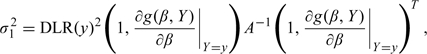
We noted earlier that ROC′(t) = DLR(y) for t = 1 − F(y). This implies that estimators of the DLR function give rise to estimators of the ROC derivative function. Estimating the ROC derivative is an important component of ROC analysis of continuous diagnostic biomarkers. Specifically, the empirical ROC curve, , is typically used for estimation, and the asymptotic distribution of − ROC(t)) is normal with mean 0 and variance

(6.1)

Therefore, CIs based on this asymptotic theory require an estimate of ROC′(t). We have previously used the ratio of kernel density estimators. However, results of our simulation studies in Table 1 suggest that estimators with better performance may be based on LR or ROC–GLM. It would be interesting to determine if this leads to better performing CIs for ROC(t) based on . Our current practice for CI construction, however, uses bootstrap resampling, thereby avoiding the need to estimate ROC′(t) (Pepe and others, 2009). More compelling motivation for estimating ROC′(t) derives from its key role in study design. In order to calculate sample size for a study based on the variance expression (6.1), an estimate of ROC′(t) must be made from pilot data. Moreover, the optimal choice of case–control ratio, λ =n_D/n, is also a function of the estimated value for ROC′(t). In particular, Janes and Pepe (2006) showed that by choosing the ratio as

the overall sample size is minimized. Having an estimate of ROC′(t) available from pilot data allows one to choose an appropriate case–control ratio for a future study.

When pilot data are available, one can estimate ROC′(t) as , where (y) is any of the 5 proposed estimators of the DLR function: DE, LR, RIDE, RILR, and ROC–GLM. We focus on the 3 rank-invariant estimators because a fundamental attribute of ROC analysis is that it is rank invariant.

6.2. Application to pancreatic cancer data

We use a pancreatic cancer data set (Wieand and others, 1989) for illustration. This was a case–control study with 90 subjects having pancreatic cancer and 51 controls who did not have cancer but had pancreatitis. Serum samples from each patient were assayed for CA-19-9, a carbohydrate antigen, which is a biomarker for cancer. We are particularly interested in the ROC curve at false-positive rate 0.2, ROC(0.2). We applied rank-invariant estimators of ROC′ to the data. Both the logistic and the ROC–GLM models were fit including linear and quadratic terms in Φ⁻¹(1 − U).

Figure 4 displays estimates of ROC′. LR and ROC–GLM produced very similar results: The estimated ROC′ curves and their CIs are almost identical. However, the nonparametric density estimator is substantially different from the other two. Observe that the magnitude of fluctuation in the estimated curve is large and that the corresponding confidence bands are extremely wide. This agrees with poor performance of density-based estimation of DLR(y) observed in the simulations summarized in Table 1.

Fig. 4.

Rank-invariant estimation of the derivative of the ROC curve for marker CA-19-9 in a pancreatic cancer study. (a) ROC′ curves and (b) 95% pointwise CIs using percentiles of the 1000 bootstrap resampled data sets. Also shown in (a) are the corresponding estimated ROC′(t) values at false-positive rate 0.2.

Table 3 shows the estimated slope values at the false-positive rate t = 0.2. The density ratio estimator is 0.404 (95% CI = (0, 1.052)), which is substantially different from the LR and ROC–GLM estimators, 0.464 (95% CI = (0.259, 0.707)), and 0.466 (95% CI = (0.254, 0.698)), respectively. Moreover, the CI based on the rank-invariant density estimator is extremely wide compared to the other estimators. The empirical estimate of ROC(0.2) is = 0.778. This along with the estimate of ROC′(0.2) gives rise to an estimate of the SD of and a CI for ROC(0.2) using the expression for σ². SDs and CIs for ROC(0.2) are also shown in Table 3.

Table 3.

Estimates of ROC′(0.2) with corresponding 95% CIs calculated as percentiles of their bootstrap distributions. Shown also are λ_opt, the estimated optimal case–control ratio for a future study of CA-19-9; (), the estimated SD of in the pilot study; and the corresponding 95% CI based on the pilot study estimate of = 0.778

Method	ROC′(0.2)		λopt	()	95% CI for ROCe(0.2)
	Estimates	95% CI
RIDE	0.404	(0.000, 1.502)	2.57	0.049	(0.681, 0.875)
RILR	0.464	(0.259, 0.707)	2.24	0.051	(0.678, 0.878)
ROC–GLM	0.466	(0.254, 0.698)	2.23	0.051	(0.678, 0.878)

Suppose we want to conduct a definitive case–control study to evaluate the diagnostic accuracy of CA-19-9 with FPR fixed at 0.2 and we have the current study of 141 observations as pilot data. The optimal case–control ratio, λ_opt, is estimated as 2.57, 2.24, and 2.23 based on the 3 rank-invariant methods. It appears that about 2.5 cases should be enrolled for each case in the definitive study. This is quite different from the case–control ratio of 1.76 used in the pilot study.

7. CONCLUDING REMARKS

This paper presents some new statistical methods to estimate the DLR function. New approaches include rank-invariant DE and rank-invariant LR. Although using densities to estimate the slope of the ROC curve and using LR to estimate the DLR function are relatively standard, their rank-invariant counterparts have not been defined previously. An advantage of rank-invariant estimators over nonrank-invariant estimators is that they can be used to compare markers.

Our methods were developed for case–control studies. However, all approaches apply to cohort studies too. Estimation methods condition on case–control status. We note that a case–control study and a cohort study with the same observations yield exactly the same DLR estimates. However, the variances of the estimates will depend on the design because the case–control ratio is subject to sampling variability in a cohort study. Therefore, when using bootstrap resampling to estimate variances, it is important to resample data sets according to the study design employed.

We adopted Gaussian kernels in applying DE methods because they are commonly used in practice. However, other kernel functions might be used, including uniform, triangle, quartic, and cosine kernels. We investigated the nonrank-invariant DE of DLR and ROC′ functions using quartic and cosine kernels for the same simulation models described here and observed that both quartic and cosine kernels yield much smaller biases but larger variances and MSEs than the Gaussian kernel (data not shown). Our overall conclusion did not change in regard to the best approach for estimating DLR and ROC′ functions: LR and ROC–GLM are much better than DE methods no matter which kernel is employed.

We have shown that the risk prediction capacity of markers can be compared using the rank-invariant DLR function, DLR(u), where u = U(Y). We did not specifically relate this to ROC curves, but there is a relationship. In particular, a marker Y₁ that is more predictive than Y₂ has higher DLR when the markers are at the high end of their scales (U(Y) low) and lower DLR when the markers are at the low end of their scales (U(Y) high). This implies that ROC₁^′(u) > ROC₂^′(u) when u is large, where u is the false positive rate. Since the ROC curves for Y₁ and Y₂ are tied down at 0 and 1, and are concave, this implies that the area under the ROC curve for Y1 is greater than that for Y₂.

FUNDING

National Institutes of Health (RO1 GM054438, UO1 CA086368) to M.S.P.

References

- Alonzo TA, Pepe MS. Distribution-free ROC analysis using binary regression techniques. Biostatistics. 2002;3:421–432. doi: 10.1093/biostatistics/3.3.421. [DOI] [PubMed] [Google Scholar]
- Baker SG. The central role of receiver operating characteristic (ROC) curves in evaluating tests for the early detection of cancer. Journal of National Cancer Institute. 2003;95:511–515. doi: 10.1093/jnci/95.7.511. [DOI] [PubMed] [Google Scholar]
- Begg CB. Advances in statistical methodology for diagnostic medicine in the 1980s. Statistics in Medicine. 1991;10:1887–1895. doi: 10.1002/sim.4780101205. [DOI] [PubMed] [Google Scholar]
- Boyko EJ. Ruling out or ruling in disease with the most sensitive or specific diagnostic test: short cut or wrong turn? Medical Decision Making. 1994;14:175–179. doi: 10.1177/0272989X9401400210. [DOI] [PubMed] [Google Scholar]
- Giard RW, Hermans J. The evaluation and interpretation of cervical cytology: application of the likelihood ratio concept. Cytopathology. 1993;4:131–137. doi: 10.1111/j.1365-2303.1993.tb00078.x. [DOI] [PubMed] [Google Scholar]
- Gu W, Pepe MS. Estimating the capacity for improvement in risk prediction with a marker. Biostatistics. 2009;10:172–186. doi: 10.1093/biostatistics/kxn025. [DOI] [PMC free article] [PubMed] [Google Scholar]
- Hanley JA. Receiver operating characteristic (ROC) methodology: the state of the art. Critical Reviews in Diagnostic Imaging. 1989;29:307–335. [PubMed] [Google Scholar]
- Huang Y, Pepe MS. Biomarker evaluation and comparison using the controls as a reference population. Biostatistics. 2009;10:228–244. doi: 10.1093/biostatistics/kxn029. [DOI] [PMC free article] [PubMed] [Google Scholar]
- Janes H, Pepe MS. The optimal ratio of cases to controls for estimating the classification accuracy of a biomarker. Biostatistics. 2006;7:456–468. doi: 10.1093/biostatistics/kxj018. [DOI] [PubMed] [Google Scholar]
- Janssens AC, Deng Y, Borsboom GJ, Eijkemans MJ, Habbema JD, Steyerberg EW. A new logistic regression approach for the evaluation of diagnostic test results. Medical Decision Making. 2005;25:168–177. doi: 10.1177/0272989X05275154. [DOI] [PubMed] [Google Scholar]
- Knudson RJ, Lebowitz MD, Holberg CJ, Burrows B. Changes in the normal maximal expiratory flow-volume curve with growth and aging. American Journal of Respiratory and Critical Medicine. 1983;127:725–734. doi: 10.1164/arrd.1983.127.6.725. [DOI] [PubMed] [Google Scholar]
- Metz CE, Herman BA, Shen JH. Maximum likelihood estimation of receiver operating characteristic (ROC) curves from continuously-distributed data. Statistics in Medicine. 1998;17:1033–1053. doi: 10.1002/(sici)1097-0258(19980515)17:9<1033::aid-sim784>3.0.co;2-z. [DOI] [PubMed] [Google Scholar]
- Moskowitz CS, Pepe MS. Quantifying and comparing the predictive accuracy of continuous prognostic factors for binary outcomes. Biostatistics. 2004;5:113–127. doi: 10.1093/biostatistics/5.1.113. [DOI] [PubMed] [Google Scholar]
- Pepe MS. A regression modelling framework for receiver operating characteristic curves in medical diagnostic testing. Biometrika. 1997;84:595–608. [Google Scholar]
- Pepe MS. The Statistical Evaluation of Medical Tests for Classification and Prediction. New York: Oxford University Press; 2003. [Google Scholar]
- Pepe MS, Cai T. The analysis of placement values for evaluating discriminatory measures. Biometrics. 2004;60:528–535. doi: 10.1111/j.0006-341X.2004.00200.x. [DOI] [PubMed] [Google Scholar]
- Pepe MS, Feng Z, Janes H, Bossuyt PM, Potter JD. Pivotal evaluation of the accuracy of a biomarker used for classification or prediction: standards for study design. Journal of the National Cancer Institute. 2008;100:1432–1438. doi: 10.1093/jnci/djn326. [DOI] [PMC free article] [PubMed] [Google Scholar]
- Pepe MS, Longton G. Standardizing markers to evaluate and compare their performances. Epidemiology. 2005;16:598–603. doi: 10.1097/01.ede.0000173041.03470.8b. [DOI] [PubMed] [Google Scholar]
- Pepe MS, Longton G, Janes H. Estimation and comparison of receiver operating characteristic curves. Stata Journal. 2009;9:1–16. [PMC free article] [PubMed] [Google Scholar]
- Scott DW. Multivariate Density Estimation: Theory, Practice, and Visualization. New York: Wiley; 1992. [Google Scholar]
- Wieand S, Gail MH, James BR, James KL. A family of nonparametric statistics for comparing diagnostic markers with paired or unpaired data. Biometrika. 1989;76:585–592. [Google Scholar]
- Zhou XH, McClish DK, Obuchowski NA. Statistical Methods in Diagnostic Medicine. New York: Wiley; 2002. [Google Scholar]