Model for Comparative Analysis of Antigen Receptor Repertoires

Abstract

In modern molecular biology one of the standard ways of analyzing a vertebrate immune system is to sequence and compare the counts of specific antigen receptor clones (either immunoglobulins or T-cell receptors) derived from various tissues under different experimental or clinical conditions. The resulting statistical challenges are difficult and do not fit readily into the standard statistical framework of contingency tables primarily due to the serious under-sampling of the receptor populations. This under-sampling is caused, on one hand, by the extreme diversity of antigen receptor repertoires maintained by the immune system and, on the other, by the high cost and labor intensity of the receptor data collection process. In most of the recent immunological literature the differences across antigen receptor populations are examined via non-parametric statistical measures of the species overlap and diversity borrowed from ecological studies. While this approach is robust in a wide range of situations, it seems to provide little insight into the underlying clonal size distribution and the overall mechanism differentiating the receptor populations. As a possible alternative, the current paper presents a parametric method that adjusts for the data under-sampling as well as provides a unifying approach to a simultaneous comparison of multiple receptor groups by means of the modern statistical tools of unsupervised learning. The parametric model is based on a flexible multivariate Poisson-lognormal distribution and is seen to be a natural generalization of the univariate Poisson-lognormal models used in the ecological studies of biodiversity patterns. The procedure for evaluating a model’s fit is described along with the public domain software developed to perform the necessary diagnostics. The model-driven analysis is seen to compare favorably vis a vis traditional methods when applied to the data from T-cell receptors in transgenic mice populations.

1 Introduction

The major feature of the adaptive immune system is its capacity to generate clones of B- and T-cells that are able to recognize and neutralize specific antigens. Both cell types recognize antigens by a special class of surface molecules called B- and T-cell receptors (TCRs). The purpose of the article is to describe in detail and illustrate with examples a new approach to analyzing and comparing TCR-type data arriving from multiple TCR repertoires, based on the use of a bivariate Poisson-lognormal distribution (BPLN) as a model of repertoire frequencies. By means of examples derived from real TCR data, we argue that under BPLN both the moment-based and the information-based parametric measures of dissimilarity yield consistent and biologically meaningful results. We also show that in all examples considered, the proposed methods outperform the standard ones in terms of their bias, variance, and the overall recognition of the frequency patterns among TCR repertoires. The methodology developed in this paper will apply to both types of receptors but, for the sake of clarity and simplicity, we describe the background and the overall problem in terms of T-cell receptors or TCRs. For a general introduction to the molecular biology of the immune system, we refer the interested reader to Janeway (2005).

A single T-cell receptor (TCR) is composed of two chains, α and β, that are assembled during T-cell differentiation. Both chains are formed by rearrangements of DNA segments: Vα and Jα for the TCRα chain and Vβ, Dβ, and Jβ for the TCRβ chain. Since there are a number of segments of each type in the genomic DNA, a great number of different α and β chains are generated. This chain diversity is further increased by the recombination process when individual nucleotides might be added or deleted at the junctional sites. The region containing these highly variable junctions is the third of the complementarity-determining regions (CDRs) that are seen crystallographically to contact an antigen and is known as the CRD3 region. Both combinatorial and insertional rearrangements result in a huge TCR repertoire that ensures that the immune system has the potential to recognize a large number of antigens. For instance, it is estimated that the number of antigen-specific TCRs that can be formed in mice exceeds 10¹⁵ (Davis and Bjorkman, 1988; Casrouge et al., 2000). For humans, it is estimated that over 10¹⁸ different TCRs can be produced with varying frequencies across various T-cell subpopulations (Arstila et al., 1999; Naylor et al., 2005), like, for example, naive and regulatory T-cells. Naive T-cells are cells that have not encountered an antigen in their lifetime, so they have never been activated, and regulatory T-cells are cells that act to suppress the activation of the immune system and thereby maintain immune system homeostasis and tolerance to self-antigens. Both subpopulations belong to the so-called The frequency of individual T-cell clones in normal individuals is very low. However, once a naive T-cell, expressing the appropriate TCR, encounters an antigen, it becomes activated and expands, forming clones of cells. This is manifested by the expression of cell surface molecules and by proliferation. T-cells responding to antigen may divide many times and increase in number > 1000 fold, forming T-cell clones expressing the same TCR (Butz and Bevan, 1998). In general, T-cells recognize only antigens bound to self proteins called the major histocompatibilty complex (MHC). Various groups of T-cells recognize antigens in the context of different sub-classes of the MHC molecules and these differences seem to have a profound effect on the diversity of the TCR repertoires (Wucherpfennig et al., 2010).

As TCR data-producing technology is becoming increasingly more reliable (Weinstein et al., 2009) and with several bioinformatics software suites available for antigen data preprocessing (Collette et al., 2003; He et al., 2005), TCR repertoire studies are becoming one of the major tools of modern immunology, providing great insight into, for example, the origin and antigen specificity of various types of T-cells (Hsieh et al., 2004; Kuczma et al., 2009b; Lathrop et al., 2008; Pacholczyk et al., 2006, 2007). As suggested by some authors (Poland et al., 2008, 2009), such knowledge could eventually lead towards individual immune system profiling and personalized vaccines. However, in order to make significant progress towards these goals, one needs to first establish a reliable statistical methodology for comparing TCRs across various repertoires of interest. Unfortunately, the extreme diversity of TCR populations, both in terms of varying frequencies and numbers of different clones, makes them particularly challenging objects for statistical analysis. Adding to this challenge is the fact that the current laborious process of TCR data collection makes it easy to seriously under-sample the data arriving from various TCR repertoires. In fact, under the popular method of single-cell sorting, single-cell RT-PCR (Freeman et al., 2009), the TCR populations are known typically to be very severely under-reported, in the sense that only a small fraction of TCR clones is examined (see, e.g., Warren et al. 2009). For that reason, the simple, non-parametric statistical methods, which are known to be sensitive to the population under-sampling bias, are only of limited use for TCR repertoire comparison studies. This includes, for instance, the popular methods based on Simpson’s diversity and Shannon’s entropy indices discussed, for example, in Ferreira et al. (2009) and Venturi et al. (2007). The more sensible approach seen in immunological studies relies on modeling diversity parametrically, assuming that all clonotypes (TCR species) are equally represented in the repertoire (Barth et al. 1985; Behlke et al. 1985). The advantage of this so-called homogeneous model is its computational and conceptual simplicity, which contributes to its wide use (cf. e.g., Casrouge et al. 2000; Hsieh et al. 2004, 2006; Pacholczyk et al. 2007, 2006). However, such a model is called into question by some empirical evidence (see, e.g., Naumov et al. 2003; Pewe et al. 2004), suggesting heavy right tails of the clonal size distributions. To account for this heterogeneity, the homogeneous model has been expanded to a variety of mixture models, typically under the assumption of the Poisson distribution of the TCR clones. These Poisson abundance mixture models (Chao, 2006) assume that each TCR variant (i.e., each clone family or clonotype) is sampled according to the Poisson distribution with a specific sampling rate, itself varying according to a prescribed parametric (mixing) distribution e.g., exponential, gamma, or lognormal (Ord and Whitmore 1986; Sepúlveda et al. 2010; Bulmer 1974). The recent detailed comparative study of Sepúlveda et al. (2010) identified one of such models, the Poisson-lognormal mixture (PLN), as particularly well suited for modeling clonal diversity. The special appeal of the PLN seems to be its capacity for an extension to a multivariate setting. Unlike many of the currently used methods, such an extension would allow for the simultaneous analysis of abundance patterns of several repertoires (Engen et al., 2002). In particular, the bivariate extension of the PLN model could be used to derive a class of dissimilarity measures for pairwise comparisons of the repertoires and for building a tree-based hierarchy, relating various TCR subpopulations. Essentially, this is the idea pursued in the current paper.

The paper is organized as follows. In the next section (Section 2) we give a brief overview of the Poisson abundance models both in univariate and multivariate (bivariate) settings. In Section 3 we discuss one method for deriving dissimilarity measures that is particularly relevant to TCR data studies. The method is useful to provide the formal definitions, in our setting, of some popular measures of dissimilarity that we later employ in our data analysis. In Section 4 we present the application of our method to two TCR datasets obtained from the populations of naive and regulatory T-cell receptors in healthy and immune-deficient mice. The first dataset was already described and analyzed by different methods in Pacholczyk et al. (2006). The second dataset is a new, previously unpublished one recently obtained from two TCR repertoires with a very low species overlap. In order to illustrate the advantages of our methodology, we analyze both datasets in detail using the clustering algorithms derived under both non-parametric and BPLN models and compare the results. For the reader’s convenience, both datasets are provided as the supplemental material available for download from XXXX. In Section 5 we provide a concise summary of our findings and offer concluding remarks, along with the description of the supplementary data files. Some elementary derivations, related to the entropy function and to the narrative of Section 3, are provided in the Appendix.

2 Poisson Models of Abundance

Poisson abundance models arrive naturally in the biodiversity studies if we assume (see, e.g., Chao 2006) that the clone (clonal species) sampling is done by a “continuous type of effort”, i.e., data is recorded as arriving from a mixture of Poisson processes in some time interval. This type of model approach can be traced back to Fisher, Corbet and Williams (Fisher et al., 1943). Consider M species labeled from 1 to M. Individuals of the i-th species arrive in the sample according to a Poisson process with a discovery rate λ_i. If the detectability of individuals can be assumed to be equal across all species (which is typically the case in a TCR repertoire), then the rates can be interpreted as species abundances (Nayak, 1991). In this sampling scheme, the sample size n (the number of individuals observed in the experiment) is a random variable. Since, given the class total n, the conditional frequencies follow a multinomial distribution with class probabilities given by relative frequencies ${\lambda }_i/{\sum }_{k=1}^M{\lambda }_k$, many estimators are shared in both the continuous-type Poisson models and the discrete-type (multinomial) models, where n is assumed to be a constant. We note here that in the case of antigen receptor data, the constant n is sometimes known (e.g., DNA sequencing data) and sometimes not known (e.g., spectratype data, see Kepler et al. 2005). In the latter case, the Bayesian framework is typically invoked and prior distributional form of n is assumed (see, e.g., Rodrigues et al. 2001; Lewins and Joanes 1984; Barger and Bunge 2008; Solow 1994). Since the present paper is motivated by the single–cell DNA sequencing data, we are assuming throughout that n is known. The extension of our model to unknown n along the lines of Rodrigues et al. (2001) is reasonably straightforward but is not pursued here.

2.1 Univariate mixture models

Since it has been generally accepted that the antigen receptor clonal size distributions have heavy right tails, to adjust for the over-dispersion, the species rates (λ₁, λ₂, …, λ_M) are typically modeled as a random sample from a mixing distribution with density f(λ; θ), where θ is a low-dimensional vector of parameters. Following the famous paper by Fisher and his colleagues (Fisher et al., 1943), many researchers have adopted a gamma density as a mixing model. Other parametric models include, among others, the log-normal (Bulmer, 1974), inverse-Gaussian (Ord and Whitmore, 1986), and generalized inverse-Gaussian (Sichel, 1997) distributions (Sepúlveda et al., 2010). An obvious advantage of such parametric models is that the inference problem reduces to estimating only a few relatively low-dimensional parameters for which the traditional estimation procedures can be typically applied. For any mixture density f(λ; θ), define p_θ(k), k = 0, 1, … as the probability that any TCR species is observed k times in the sample, that is

$$p_{\theta }(k)={\int }_0^{\infty }[{\lambda }^k{e}^{-\lambda }/k!]f(\lambda ;\mathit{\theta })d\lambda k=0,1,\dots .$$ (2.1)

Denoting by f_k (k = 1, 2, …, n) the number of receptor species observed exactly k-times in the sample we have E(f_k) = Mp_θ (k). Setting D = Σ_k f_k, the likelihood function for M and θ can be written as

$$L(M,\mathit{\theta }\mid \{f_k\})=\frac{M!}{(M-D)!{\prod }_{k\ge 1}(f_k!)}{[p_{\theta }(0)]}^{M-D}\prod _{k\ge 1}{[p_{\theta }(k)]}^{f_k}.$$

The (unconditional) MLEs for M and θ and their asymptotic variances are obtained based on the above likelihood, which, as we can see, depends on the data only through the observed values of {f_k}. The likelihood can be factored as

$$L(M,\mathit{\theta }\mid \{f_k\})=L_b(M,\mathit{\theta }\mid D)L_c(\mathit{\theta }\mid \{f_k\},D)$$

where L_b(M, θ|D) is a likelihood with respect to D, a binomial (M, 1 − p_θ (0)) variable, and L_c(θ|{f_k}, D) is a (conditional) multinomial likelihood with respect to {f_k; k ≥ 1} with cell total D and zero-truncated cell probabilities p_θ (k)/[1 − p_θ (0)], k ≥ 1, i.e.,

$$L_c(\mathit{\theta }\mid \{f_k\},D)=\frac{D!}{{\prod }_{k\ge 1}(f_k!)}\prod _{k\ge 1}{\left[\frac{p_{\theta }(k)}{1-p_{\theta }(0)}\right]}^{f_k}.$$ (2.2)

The MLE of θ obtained from this likelihood can be regarded as a (conditional) empirical Bayes estimator if we think of the mixing distribution as a prior distribution having unknown parameters that must be estimated (see Rodrigues et al. 2001 for further reference).

2.2 Extension to bivariate models

As we shall see in the next section, for the purpose of comparing multiple TCR repertoires simultaneously, it is of interest to also consider multivariate models of abundance. For the sake of our discussions below we focus on the bivariate models but the modifications for higher dimensions are rather straightforward. In direct analogy with the notation of the previous section, we now define p_θ (k, l) to be the probability that any TCR species (i.e., a TCR clone) is present k times in the sample from the first population (repertoire) and l times in the sample from the second one. For simplicity, assume that we have the same M species in both populations. However, this is an assumption of convenience only, since the species that are present in one but not the other repertoire may be considered as arriving with joined probability p_θ (k, 0) or p_θ (0, l) for some k, l > 0. Accordingly, the value M could be viewed as a number of different bivariate species of TCRs with marginally unequal counts.

Let f_k,l be the empirical count and set now D = Σ_k,l≥0 f_k,l (assuming f_0,0 = 0). Let f (λ₁, λ₂; θ) be the bivariate mixture distribution. The likelihood formulae from the previous section extends to the bivariate case as

$$L(M,\mathit{\theta }\mid \{f_{k,l}\})=\frac{M!}{(M-D)!{\prod }_{k,l\ge 0}(f_{k,l}!)}{[p_{\theta }(0,0)]}^{M-D}\prod _{k,l\ge 0}{[p_{\theta }(k,l)]}^{f_{k,l}}.$$

where

$$p_{\theta }(k,l)={\int }_0^{\infty }[{\lambda }_1^k{e}^{-{\lambda }_1}{\lambda }_2^l{e}^{-{\lambda }_2}/(k!l!)]f({\lambda }_1,{\lambda }_2;\mathit{\theta })d{\lambda }_{1}d{\lambda }_{2}k,l=0,1,\dots .$$ (2.3)

Note that, as before, E(f_k,l) = Mp_θ (k, l). The likelihood function for M and θ can be again factored as

$$L(M,\mathit{\theta }\mid \{f_{k,l}\})=L_b(M,\mathit{\theta }\mid D)L_c(\mathit{\theta }\mid \{f_{k,l}\},D)$$

where, in obvious analogy with (2.2), L_b(M, θ |D) is now a likelihood with respect to D, a binomial variable with parameters (M, 1 − p_θ (0, 0)), and L_c(θ |{f_k,l}, D) is a (conditional) multinomial likelihood with respect to {f_k,l, k + l > 0} with cell total D and the bivariate, zero-truncated cell probabilities {p_θ (k, l)/[1 − p_θ (0, 0)]}_k,l, k + l > 0, i.e.,

$$L_c(\mathit{\theta }\mid \{f_{k,l}\},D)=\frac{D!}{{\prod }_{k,l\ge 0}{f}_{k,l}!}\prod _{k\ge 1}{\left[\frac{p_{\theta }(k,l)}{1-p_{\theta }(0,0)}\right]}^{f_{k,l}}.$$ (2.4)

3 Diversity Analysis and Clustering

When studying the evolution of TCR species, it is of interest to compare their diversity, by which we mean herein (cf. Section 1) the clonal size distribution {p_θ (k)} and the species number M. Such repertoire diversity comparisons are of great relevance, for instance, in clinical studies, where the quantity of interest is the “divergence” of multiple observed TCR repertoires from the control. The individual repertoires of antigen receptors can be then characterized in terms of their divergence from the control (Chen et al., 2003; Komatsu et al., 2009; Pacholczyk et al., 2007, 2006). Under our adopted definition, the TCR repertoire diversity is completely determined by the parameters (M, θ). This agrees with the original concept of “species diversity” known from the field of ecology where the term itself relates both to the number of species (richness) and to their apportionment within the sequence (evenness or equitability, see Sheldon 1969). A sensible method of comparing the diversity of multiple repertoires simultaneously is based on a concept of (pairwise) diversity dissimilarity measure and the hierarchical clustering induced by it. The hierarchical clustering, which we discuss in more detail below, is one of the many modern methods of analyzing patterns in high-dimensional data on the grounds of the so-called unsupervised statistical learning theory (cf., e.g., Hastie et al. 2001), a very dynamically developing area of modern statistics.

3.1 Diversity dissimilarity measures

Assume that the overall “similarity” between a pair of TCR repertoires with respective clonal abundance distributions p and q is quantified by some non-negative function Q(p, q), referred to as the similarity index or similarity measure. Since typically the samples from the joined distribution (frequency) of abundance are not available in data collected from TCR repertoires, some of the crude similarity indices are based simply on the joined TCR species presence/absence data, i.e., the number of TCR species shared by two samples and the number of species unique to each of them (see discussion in Legendre and Legendre, 1998). Examples of such indices are the classical Jaccard index and the closely related Sørensen index, the two oldest and most widely used similarity indices in ecological biodiversity studies (Magurran, 2005). One of the advantages of the Poisson mixture model described in the previous section is that it allows for defining meaningful indices incorporating pairwise comparisons of the TCR species based on the joined distribution of abundance. As representative examples of such indices, we consider here the Morisita-Horn index () (Magurran, 2005), the mutual information criterion (), which is a special case of a Kullback-Leibler divergence (see, e.g., Koski, 2001), and the overlap index () introduced by Smith et al. (1996). All of these indices give rise to the corresponding measures of dissimilarity concentrated on the unit interval with the perfect correlation (or complete overlap) between the frequency distributions yielding the value zero. Indeed, they are all seen as special cases of the following general construction. For any bivariate probability distribution p_θ with corresponding marginal distributions $p_{\theta }^{(1)}$ and $p_{\theta }^{(2)}$, consider a similarity index $\mathcal{Q}(p_{\theta }^{(1)},p_{\theta }^{(2)})$ satisfying

$$0\le \mathcal{Q}(p_{\theta }^{(1)},p_{\theta }^{(2)})\le \frac{\mathcal{Q}(p_{\theta }^{(1)},p_{\theta }^{(1)})+\mathcal{Q}(p_{\theta }^{(2)},p_{\theta }^{(2)})}{2}$$ (3.1)

with the right bound attained when $p_{\theta }^{(1)}=p_{\theta }^{(2)}$. Then the corresponding (normalized) -induced measure of dissimilarity between the pair ( $p_{\theta }^{(1)},p_{\theta }^{(2)}$) may be defined as

$$\mathcal{D}(p_{\theta }^{(1)},p_{\theta }^{(2)})=1-\frac{2\mathcal{Q}(p_{\theta }^{(1)},p_{\theta }^{(2)})}{\mathcal{Q}(p_{\theta }^{(1)},p_{\theta }^{(1)})+\mathcal{Q}(p_{\theta }^{(2)},p_{\theta }^{(2)})}.$$ (3.2)

To obtain the Morisita-Horn dissimilarity index (), we take in (3.2) =

$${\mathcal{Q}}_{MH}(p_{\theta }^{(1)},p_{\theta }^{(2)})=\sum _{k,l\ge 1}kl{p}_{\theta }(k,l),$$ (3.3)

which obviously satisfies (3.1) for any non-negative random variables. A closely related correlation-based dissimilarity index is obtained when we take = with

$${\mathcal{Q}}_{\rho }(p_{\theta }^{(1)},p_{\theta }^{(2)})=\mid \sum _{k,l\ge 0}\stackrel{\sim }{k}\stackrel{\sim }{l}{p}_{\theta }(k,l)\mid ,$$ (3.4)

where k̃ = (k − m₁)/s₁ and l̃ = (l − m₂)/s₂ and m_i and s_i are, respectively, mean and standard deviation of $p_{\theta }^{(i)}$, i = 1, 2. In this case the inequality (3.1) simply asserts that 0 ≤ ≤ 1.

A popular dissimilarity measure, which we shall denote here by is obtained by averaging conditional probabilities of the presence of individual receptor species in both samples, given its presence in one. The measure was introduced by Smith et al. (1996) to quantify the “overlap” between repertoires, and is obtained by taking the following similarity index.

$${\mathcal{Q}}_{OV}(p_{\theta }^{(1)},p_{\theta }^{(2)})=\frac{{\sum }_{k,l>0}{p}_{\theta }(k,l)}{2}\left(\frac{1}{{\sum }_{k>0}{p}_{\theta }^{(1)}(k)}+\frac{1}{{\sum }_{l>0}{p}_{\theta }^{(2)}(l)}\right),$$ (3.5)

which again trivially satisfies (3.1).

Finally, in order to obtain the mutual information dissimilarity index () we take in (3.2) = where

$${\mathcal{Q}}_{MI}(p_{\theta }^{(1)},p_{\theta }^{(2)})=\sum _{k,l\ge 0}{p}_{\theta }(k,l)log\left(\frac{p_{\theta }(k,l)}{p_{\theta }^{(1)}(k)p_{\theta }^{(2)}(l)}\right).$$ (3.6)

The fact that the above function satisfies (3.1) is shown in the appendix. Note that all the above similarity indices, , , , and (and thus also their corresponding dissimilarity measures), depend on the underlying mixing distribution parameter θ but not explicitly on the species number M. This is desirable since the quantity M is typically unknown and difficult to estimate, due to often very severe undersampling of the TCR repertoires (cf., e.g., Sepúlveda et al. 2010). In the parametric setting considered here, if needed, the value of M may be estimated (aposteriori) by either of the estimates

$${\widehat{M}}_1=D/(1-p_{\widehat{\theta }}(0,0))$$ (3.7)

$${\widehat{M}}_2=\sum _{k,l\ge 0,k+l>0}{f}_{k,l}/p_{\widehat{\theta }}(k,l)$$ (3.8)

whose close numerical agreement usually indicates a robust fit of the bivariate parametric mixture model. Note that M̂₂ is simply a parametric version of the Horvitz-Thompson estimator (Horvitz and Thompson, 1952).

3.2 Hierarchical clustering

For a given pairwise dissimilarity measure of TCR repertoires, it is a standard unsupervised statistical learning approach to simultaneously compare N repertoires in terms of by means of building hierarchical clusters that are graphically represented by dendrograms or “tree diagrams”. In such a hierarchical clustering procedure, the TCR data are not partitioned into a particular cluster in a single step. Instead, as the name suggests, a hierarchical structure is produced in which the clusters at each level of the hierarchy are created by merging clusters at the next lower level. The main advantage of the hierarchical clustering approach lies in the fact that no cluster number needs to be specified in advance. Hierarchical clustering is performed via either agglomerative methods, which proceed by a series of fusions of the N objects into groups, or divisive methods, which separate objects successively into finer groupings. Agglomerative techniques are more commonly used, and this is the method we consider below for TCR repertoires. The extent to which the hierarchical structure produced by a den-drogram actually represents the data itself can be judged by the cophenetic correlation coefficient. This is the correlation between the N(N − 1)/2 pairwise observation dissimilarities d_ii′ input to the clustering procedure and their corresponding cophenetic dissimilarities c_ii′ derived from the dendrogram. The cophenetic dissimilarity c_ii′ between two observations (i, i′) is the value of the intergroup dissimilarity at which observations i and i′ are first joined together in the same cluster. The cophenetic correlation coefficient may be used to assess to what extent various dissimilarity measures reflect the true pattern of the data, with high positive values (above .9) indicating good agreement.

For a general introduction to clustering and unsupervised learning, the interested reader is referred to Chapter 14 in the popular monograph of Hastie et al. (2001).

3.3 Poisson-lognormal model

Whereas there are many possible models of parametric bivariate mixture, the recent studies in Engen et al. (2002) and Sepúlveda et al. (2010) seem to indicate that lognormal mixing distributions may be often an appropriate choice for TCR repertoire modeling. In that spirit we consider herein a bivariate model based on log-binormal variates. Under the assumption of random sampling, the number of individuals sampled from a given receptor species with abundance λ is Poisson distributed with mean ωλ where the parameter ω expresses the sampling intensity (see, e.g., appendix of Engen et al. 2002). If we assume that ln λ is normally distributed with mean μ and variance σ² among TCR species, then the vector of individuals sampled from all M species constitutes a sample from the Poisson lognormal distribution with parameters θ = (μ + ln ω, σ²), where μ and σ² are the mean and variance of the log abundances. For ω = 1 the corresponding mass function is of the general form (2.1) and may be written as

$$p(k;\mu ,{\sigma }^2)={\int }_{-\infty }^{\infty }{g}_k(\mu ,\sigma ,u)\phi (u)du$$ (3.9)

where φ(·) is a standard normal density function and

$$g_k(\mu ,\sigma ,u)=\frac{exp[u\sigma k+\mu k+e^{-(u\sigma +\mu )}]}{k!},k\ge 0$$

is the re-parametrized Poisson distribution. Similarly, when we consider pairs of counts of individual receptors from two different repertoires, we may think of them as a random sample (of size M) from the bivariate Poisson-lognormal distribution (BPLN), with the probability mass function given as in (2.3). Since the marginal sampling intensities (ω) may be incorporated into the BPLN mean vector, we take ω = 1 throughout the remainder of the paper, making a tacit assumption that the marginal sample sizes (Σ_k>0 f_k) are of comparable magnitude. This turns out to be the case for the TCR datasets discussed in the next section, where we assume that the pairs of log abundances among species have the binormal distribution with parameters (μ₁, μ₂, σ₁, σ₂, ρ). Under the assumed Poisson sampling, this particular specification gives rise to the BPLN distribution, a member of a general class of the multivariate Poisson distributions described, for instance, in Aitchison and Ho (1989). If we let φ(u, v; ρ) denote the normal bivariate density with correlation coefficient ρ, zero means and unite variances, then the distribution of the BPLN random variable is given in terms of the bivariate probability mass function $p_{\theta }(k,l)=p(k,l;{\mu }_1,{\mu }_2,{\sigma }_1^2,{\sigma }_2^2,\rho )$ for k, l ≥ 0 where

$$p(k,l;{\mu }_1,{\mu }_2,{\sigma }_1^2,{\sigma }_2^2,\rho )={\int }_{-\infty }^{\infty }{\int }_{-\infty }^{\infty }{g}_k({\mu }_1,{\sigma }_1,u)g_l({\mu }_2,{\sigma }_2,v)\phi (u,v;\rho )dudv.$$ (3.10)

From the above formula it follows in particular that both marginals of BPLN are the univariate Poisson-lognormal distributions (3.9) with respective parameters (μ_i, ${\sigma }_i^2$) (i = 1, 2). Since M is usually unknown, when fitting the model we only consider the number of individuals for the observed receptor species and thus the distribution of the number of observed individual receptors follows the zero-truncated BPLN distribution with probability mass function

$$\frac{p(k,l;{\mu }_1,{\mu }_2,{\sigma }_1^2,{\sigma }_2^2,\rho )}{1-p(0,0;{\mu }_1,{\mu }_2,{\sigma }_1^2,{\sigma }_2^2,\rho )}.$$ (3.11)

The maximum-likelihood estimators (MLEs) of the parameters of this distribution were discussed, e.g., in Bulmer (1974) and more recently in Karlis (2003) and Engen et al. (2002). The latter approach is conveniently implemented in the freely available R package poilog (R Development Core Team, 2009), which we have used in the current paper to perform all the necessary parameter fitting. In our setting, the model parameters were calculated from the multinomial conditional likelihood function (2.4), where the truncated probability quantity p_θ (k, l)/(1 − p_θ (0, 0)) was given by (3.11).

Under the assumed BPLN model, the measures of dissimilarity may be computed either directly or by Monte-Carlo approximations. Denoting the means of the BPLN marginals by

$${\alpha }_i=exp[{\mu }_i+{\sigma }_i^2/2]i=1,2,$$ (3.12)

the moment-based dissimilarity measures and are given by

$${\mathcal{D}}_{MH}=1-\frac{2{\alpha }_1{\alpha }_{2}exp[\rho {\sigma }_1{\sigma }_2]}{{\alpha }_1(1+{\alpha }_{1}exp[{\sigma }_1^2])+{\alpha }_2(1+{\alpha }_{2}exp[{\sigma }_2^2])}$$ (3.13)

$${\mathcal{D}}_{\rho }=1-\frac{2{\alpha }_1{\alpha }_2(exp[\rho {\sigma }_1{\sigma }_2]-1)}{\sqrt{{\alpha }_1(1+{\alpha }_1(exp[{\sigma }_1^2]-1))}\sqrt{{\alpha }_2(1+{\alpha }_2(exp[{\sigma }_2^2])-1)}}$$ (3.14)

where in (3.14) the quantities

$${\alpha }_i(1+{\alpha }_i(exp[{\sigma }_i^2]-1))i=1,2$$ (3.15)

are seen to be the marginal variances of the BPLN distribution. The formulae (3.13–3.14) provide for a convenient way of estimating the dissimilarities and from the data simply by replacing the unknown distribution parameters by their sample maximum likelihood estimates calculated, for instance, by using the numerical algorithms implemented in the “poilog” R-package. In view of the truncation (3.11) of the observed distribution, the MLE inference is preferred for the PBPLN-based dissimilarity measures, due to the intractability and/or poor performance of the other types of estimates (like, for instance, the method of moments). Interestingly, the measure remains unchanged under this truncation, and consequently, the empirical, moment-based estimate of is available.

Unfortunately, due to the fact that the mass function (3.10) is not available in a closed form, there are no closed, MLE-based formulae for the indices , . These indices are typically approximated by the Monte-Carlo-based bootstrap procedure resampling from the model with estimated parameters. The bootstrap methods are then often used to derive confidence intervals and standard errors of such parameter estimates. The general justification for such derivations is provided, e.g., in Gill et al. (2009) and Rempala and Szatzschneider (2004). The reader is referred to Efron and Tibshirani (1997) for a general introduction to the theory and practice of statistical bootstrap, which is also essential in our modeling approach and in the data analysis described below.

4 Application to TCR Repertoire Data

In this section we illustrate the parametric inference on T-cell receptor data based on the BPLN model and the associated pairwise dissimilarity measures. For the sake of comparison, we also perform the more standard, non-parametric analysis of the same data. Two datasets of different T-cell families referred to commonly as CD4+ and CD8+ are considered. Both sets are derived from two types of a genetically-engineered (TCR-mini) mice: the “wild” type with genetically restricted TCR repertoire and unaltered repertoire of self antigens bound to class II MHC, and the “Ep” (B63VJEp) mice that in addition to restricted TCR repertoire also express only single, covalently linked to MHC, Ep peptide (Pacholczyk et al., 2006). In addition, both mice types express natural class I MHC/peptide complexes. The description of the transgenic TCR-mini mouse was already given in the recent work by Pacholczyk et al. (2007). Briefly, the TCR-mini mouse is a new generation, TCR transgenic mouse in which all T-cells express one pre-specified TCRβ chain (specifically, the chain Vβ14Dβ2Jβ2.6), and the unique TCRα mini locus. This mini locus allows only for restricted rearrangements of a single Vα2.9 segment to one of the two Jα (Jα26 and Jα2) segments. The mouse has no other loci encoding TCRα chains, and therefore its entire repertoire of TCRs is derived from the artificially introduced TCRα mini locus, resulting in a greatly reduced TCRs diversity. For these reasons the TCR-mini mouse is considered a good biological model for analyzing TCR repertoire patterns with relatively small samples of sequenced clones (Pacholczyk et al., 2006).

4.1 Analysis of CD4+ data

For the purpose of testing our statistical model, two subpopulations of CD4+ T-cells were collected representing, respectively, regulatory (TR) and naive (TN) T-cells (where the TR cells are defined as those expressing the additional marker Foxp3). In addition, these two subpopulations of CD4+ T-cells were isolated either from (1) the peripheral lymph nodes or (2) the thymus, giving us a total of eight TCR populations differing by the animal type, T-cell type, and tissue location. In the thymus, gross of CD4+ T-cells undergo development and in the lymph nodes CD4+ T-cells are retained unless activated by specific antigen and therefore two markedly different patterns of clonal abundance in these organs are generally expected. Additionally, because the “Ep” mice express only a single class II MHC/peptide complex, their diversity of the CDR3 region of the TCRα chain is drastically reduced in comparison to TCR-mini wild-type mice. Due to these pronounced biological differences between the repertoires, the dataset seems uniquely suitable for testing the performance of various statistical comparison methods.

The TCR data from both types of mice was collected as follows (for more details on a similar data harvesting procedure, see also Freeman et al. 2009). Using fluorescence activated cell sorting, populations of T-cells from different organs were single-cell-sorted into individual wells on 96-well plates and their unique CDR3 regions of their TCRα chain were amplified using single-cell RT-PCR (see, e.g., Kuczma et al. 2009a). Following this amplification, the CDR3 regions were sequenced and analyzed, providing the distribution of these regions in native subpopulation(s) of T-cells. This type of procedure has been widely considered to be one of the most reliable methods to harvest T-cell repertoires (Luczynski et al., 2007). Single T-cells can be separated from the cell suspension or isolated from tissue sections. Both the α and the β chains can be amplified and sequenced to provide unambiguous identification of T-cell clones. This method avoids the problems of skewed PCR amplification and varying TCR mRNA expression in different cells. Its obvious drawback is the under-sampling issue alluded to already in Section 1: a very large number of cells need to be analyzed to ensure detection of rare clones and to provide a global representation of the T-cell repertoire. We note that with the availability of the next generation sequencing technology (Wong et al., 2007), the large number of single cell RT-PCRs could be replaced with the high throughput PCR from a heterogeneous population of T-cells. However, at its current stage the technology is not yet recommended for repertoire analysis due to difficulties of matching specific TCRα and TCRβ chains when amplified simultaneously. In addition, there is also a high risk of count bias due to the skewed amplification process in high throughput data, which tends to overexpress the most dominant DNA sequences and underexpress (or even remove) the rare ones.

The complete dataset consisting of all sequenced receptors in eight repertoires (for a total of 1174 different clonotypes) is provided as supplementary material, which may be downloaded from the site XXXX. The pictorial summary of the empirical frequencies for each of the eight TCR repertoires considered is presented in Figure 1 as a set of eight bar plots. The bars in each plot correspond to the observed frequencies (some possibly zero) of the different clonotypes observed (sequenced) in the respective population. The ordering of the TCR sequences remains the same across plots so as to allow for direct comparison. Further summary statistics of the data are provided in Table 1 as follows. In the notation of Subsection 2.1 let $D_i={\sum }_{k>0}{f}_k^{(i)}$ and $n_i={\sum }_{k}k{f}_k^{(i)}$, where $f_k^{(i)}$ is the number of clonotypes observed k times in repertoire i, i = 1, … 8. The observed values of D_i and n_i based on all the observed clonotypes are presented in Table 1. The observed overlap between (i.e., presence in both) the TN and TR populations from combined tissues was reported in Pacholczyk et al. (2007) as at least 39% when considering only the “frequent species”, defined as those with a likely sufficiently high frequency (see equations (1) and (2) and Figure 1B in Pacholczyk et al. 2007). However, when considering all the identified clonotypes, this percentage drops considerably to about 9% of the common clones observed in Ep populations and about 5% in wild-type populations.

Figure 1. Marginal empirical counts for individual clonotypes in TCR-mini mice dataset.

The empirical frequencies for each TCR clonotype in eight repertoires are presented as bar plots, with each bar corresponds to the observed frequency (possibly zero) of a particular clone sequence observed in the respective population. The ordering of the clone sequences remains the same across all bar plots so as to allow for direct comparison. The maximal empirical count observed was 42, but for better readability, all the counts are truncated at 16.

Table 1.

The summary statistics D_i and n_i for Ep (TCR-restricted) and Wt (wild-type) mice repertoires in each population of the regulatory (TR) and naive (TN) T-cells from the lymph nodes (1) and thymus (2). The overlap between pooled TR and TN repertoires was found to be about 9% in Ep and 5% in Wt.

	Ep				Wt
	TN1	TR1	TN2	TR2	TN1	TR1	TN2	TR2
ni	206	295	207	194	378	415	346	340
Di	108	170	143	131	177	295	177	266

4.1.1 Parametric analysis

In order to assess the usefulness of a proposed parametric method of TCR data modeling, we have first generated the BPLN model-based estimates of the dissimilarity matrix for the eight TCR repertoires using, separately, each of the four dissimilarity measures of the general form (3.2) described in Section 3. For the moment-based dissimilarities and we have used the explicit formulae (3.13) and (3.14) whereas for the remaining two measures and we have directly approximated the quantities $p(k,l;{\mu }_1,{\mu }_2,{\sigma }_1^2,{\sigma }_2^2,\rho )$ given by (3.10) and subsequently used the parametric bootstrap procedure to produce the empirical approximations of dissimilarities. In all cases the BPLN distribution parameters were estimated by the maximum likelihood estimators (MLEs) computed by maximizing the conditional multinomial likelihood function (2.4) based on the zero-truncated probabilities (3.11). In principle, one could use the conditional likelihood of multivariate Poisson-lognormal distribution directly, to estimate all of the parameters simultaneously, however, due to the complicated form of the resulting mixture probabilities, we have deemed that approach to be too unreliable numerically. On the other hand, the iterative bivariate model fitting (fitting one BPLN model at a time, conditionally on the remaining repertoires and iterating until convergence) was seen to be a reasonably fast and numerically stable procedure, yielding a set of estimates consistent with marginally MLE-fitted parameters, regardless of the order in which conditioning was performed.

The results of the conditional MLE procedure are partially summarized in Table 2 where the estimates of the μ and σ² parameters for Poisson-lognormal abundance distributions for the eight repertoires are reported along with the corresponding confidence intervals obtained via the parametric bootstrap bias-corrected percentile method (see, e.g., Rempala and Szatzschneider 2004 for details on bootstrap-based interval estimation). Note that the parameters μ and σ² are related to the marginal estimates of means and variances of the Poisson-lognormal variates by the formulae (3.12) and (3.15), respectively. In order to conserve space, the estimates of the BPLN correlation coefficients are not shown as they are similar in relative values to the moment-based dissimilarities summarized in Figure 3. We note that the marginal values of the repertoire-specific parameters in both types of repertoires (wild-type and Ep) were found to be of similar magnitude (with estimated values of μ parameters between −4.5 and −2.9 and σ² parameters between 1.3 and 2). Overall, the numerical values of the parameters indicated smaller Poisson-lognormal means for the restricted-repertoire mice as compared with the wild-type. Additionally, the naive T-cell repertoires generally seemed to have smaller means and larger variances of the mixing log-normal distributions than the regulatory T-cell repertoires.

Table 2.

Maximum likelihood estimates of the means and variances of the log-abundances in Ep (TCR-restricted) and Wt (wild-type) mice repertoires along with bias-corrected, two-sided 95% confidence bounds generated via parametric bootstrap. In each population the regulatory (TR) and naive (TN) T-cells from (1) lymph nodes and (2) thymus are considered.

	Ep				Wt
	TN1	TR1	TN2	TR2	TN1	TR1	TN2	TR2
μ̂	−4.54	−3.90	−3.58	−3.80	−3.70	−2.97	−3.55	−2.90
95% Lo	−5.37	−4.81	−4.59	−4.71	−4.86	−3.77	−4.46	−3.81
95% Up	−3.31	−2.43	−2.40	−2.54	−2.59	−2.13	−2.38	−1.87
σ̂ 2	2.03	1.93	1.66	1.70	1.99	1.48	1.84	1.31
95% Lo	1.60	1.52	1.17	1.21	1.61	1.15	1.46	0.90
95% Up	2.36	2.29	1.99	2.02	2.47	1.74	2.15	1.70

Figure 3. Repertoire dendrograms and their confidence bounds obtained under BPLN model in CD4+ dataset.

Dendrograms for hierarchical clustering and their corresponding confidence intervals obtained using agglomerative clustering and a complete link for eight repertoires of naive and regulatory TCRs derived from (1) lymph nodes and (2) thymus in wild-type and Ep TCR-mini mice (cf. Figure 1). Top (A) panels: (A1) – clustering using Morisita-Horn dissimilarity measure given by (3.3); (A2) – bootstrap estimate of the one-sided 95% confidence interval (CI) of the Frobenius norm of the -dissimilarity matrix; (A3) – dendrogram corresponding to the upper bound of the one-sided 95% CI -dissimilarity matrix. Bottom (B) panels: hierarchical clustering according to the parametric mutual information dissimilarity measure given by (3.6).

As in Engen et al. (2002), the goodness-of-fit statistics were calculated for the bivariate marginal fit by resampling the conditional likelihood statistic (2.4). In all cases the differences between the bivariate data and fitted models were not-significant (all p-values <.05) as measured by the bootstrap tests, indicating a reasonably good fit of the parametric distributions to the (zero-truncated) abundance data. In addition to the goodness-of-fit testing, we have also performed qualitative comparisons of BPLN model versus data via smoothed heat-map plots (Anderes et al., 2009). One example of such a comparison is provided in Figure 2, where the smoothed heat-map illustrates both true and model-generated bivariate abundance distributions of wild-type naive and regulatory TCR repertoires derived from thymus (i.e., Wt TN2 and Wt TR2). For better visualization, the smoothing of the intensities was performed via the Gaussian kernel density smoother truncated to its non-negative support (see, e.g., Sheather and Jones 1991).

Figure 2. Model generated vs observed pairs of frequency data for CD4+ T-cells.

Left panel: kernel-density-smoothed heat-map of joined frequency data of thymus naive (y-axis) and thymus regulatory (x-axis) TCR repertoires in wild-type mice (i.e., Wt.TR2 vs Wt.TN2). Right panel: kernel-density-smoothed heat-map for the same size sample simulated from the distribution of BPLN random variable fitted to the data. Increased brightness indicates higher frequency. The smoothed intensities are truncated to the nonnegative support of the original distributions for better visualization.

The results of hierarchical clustering analysis of the eight mice TCR repertoires under and are presented in Figure 3. Panels A1 and B1 show the dendrograms obtained by agglomerative hierarchical clustering with a complete link function (see, e.g., Hastie et al. 2001, Chapter 14 for a definition) using (top) and (bottom) as the dissimilarity measures. Both dendrograms indicate a very good mutual agreement of the cluster hierarchical structure and the correct final classification of the eight repertoires in terms of the experimental condition (TCR-restricted vs wild-type) as well as the repertoire type (naive or regulatory) and tissue type (thymus vs lymph nodes). Almost identical dendrograms (not shown) were also produced by applying the remaining two measures discussed, namely and . Figure 3, panels A2 and B2, illustrate the bootstrap approximations to the distribution of the Frobenius norm (see, e.g., Golub and Van Loan 1996 for more on matrix norms) of the dissimilarity matrix [ (i, j)] (top) and [ (i, j)] (bottom) (1 ≤ i, j ≤ 8), with the one-sided 95% confidence bound marked with a vertical line. Panels A3 and B3 show the dendrograms corresponding to the dissimilarity matrices at the upper bound of the corresponding 95% confidence intervals (marked as vertical lines in the central panels). The fact that the left and right dendrograms in the top and bottom panels have identical relative hierarchies indicates a strong robustness of the hierarchical clustering against the fluctuations of both and . The similar robustness was also seen for , and . This empirical agreement between the entries of the dissimilarity matrices generated under the BPLN model using four different dissimilarity measures , , and is further illustrated in Figure 4 where the pairwise loess regressions (Cleveland and Devlin, 1988) of the entries of the dissimilarity measures on each other are presented. The plots clearly indicating the monotone relationships (almost a linear one between the first three measures), as quantified by the corresponding Spearman’s correlation coefficients.

Figure 4. Pairwise comparison of dissimilarities under BPLN model in CD4+ dataset.

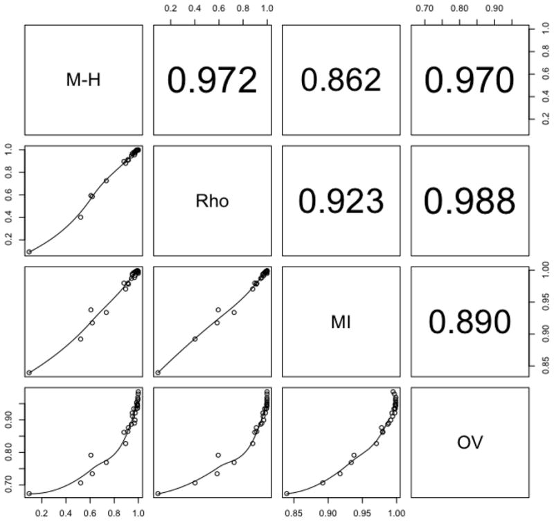
Below-diagonal panels: pairwise dissimilarities plots obtained under BPLN models fitted to mice data for the four different measures discussed in Section 3.1. Local (loess) regression curves were added to the plots for better readability. Above-diagonal panels: Spearman’s correlation coefficient values for the corresponding scatter plots.

For some additional, more quantitative assessment of the performance of and , we have also calculated their respective cophenetic correlations (see Section 3.2). The empirical values of the cophenetic correlation coefficients for (cc_MH) and (cc_MI) along with their bootstrap confidence intervals are given in Table 3. In both cases the high values of the correlations indicate the internal consistency of and with their corresponding dendrogram structures.

Table 3.

The estimated cophenetic correlation coefficients ${\widehat{cc}}_{MH}$ and ${\widehat{cc}}_{MI}$ for the dissimilarity measures and under the BPLN model. The bias-corrected bootstrap percentile method was used to derive the 95% confidence intervals.

	Value	95% Lo	95% Up
${\widehat{cc}}_{MH}$	0.970	0.901	0.984
${\widehat{cc}}_{MI}$	0.939	0.877	0.966

For the final analysis of the CD4+ dataset under the BPLN model, we have also computed the species richness estimates (3.7) and (3.8) for each pair of repertoires (for a total of 28 pairwise comparisons) and averaged the result to obtain a pooled estimator of the ratio D/M, which was found to be .09 with the 95% confidence interval of (.06, .11). These values suggest a much more severe under-sampling of the TCR populations than the traditional non-parametric estimator of Good (1953) given by f₁/D ≈ .25 (where now f₁ and D are computed from the pooled repertoire data).

The overall results of the hierarchical clustering analysis summarized in Figure 3 indicate that the BPLN model correctly identifies the dissimilarity pattern of the eight TCR repertoires considered. According to the model, the discriminating factors between various TCR populations are, in order of importance, (i) the type of animal (Wt vs Ep), (ii) the type of CD4+ cell (TN or TR), and (iii) the type of tissue (thymus or lymph nodes). These findings are consistent with our current biological knowledge about CD4+ cells, and in particular, confirm that the regulatory CD+ T-cells that express the Foxp3 transcription factor (TR) have a more diverse repertoire of TCRs and fewer dominant clones than the CD4+ T-cells that do not express Foxp3 (TN). This difference is seen to persist across both mouse types.

Whereas the similar conclusions were reached in Pacholczyk et al. (2007), the ones summarized in Figure 3 go much further in two crucial aspects. Firstly, since the hierarchical representation depicted in Figure 3 allows for quantitative description of the interplay between the discriminating factors (i)–(iii), the current results are fully quantitative and not merely qualitative, allowing therefore for much more detailed repertoire comparisons. For instance, it is clear from the dendrograms in Figure 3 that the average (complete) dissimilarity between TN and TR groups is larger in the wild-type populations that in the Ep ones. These kinds of subtleties would be impossible to uncover via the descriptive methods used in Pacholczyk et al. (2007). Secondly, and perhaps most importantly, our analysis outlined in Figure 3 indicates that, after properly accounting for both data under-sampling (i.e., the observed distributions zero-truncation) and unequal marginal sample sizes, the discriminating factors (i–iii) are statistically significant. A similar statement does not follow from the somewhat more qualitative analysis performed in Pacholczyk et al. (2007).

4.1.2 Non-parametric analysis

In order to further examine the results of our parametric analysis of the TCR repertoires, we have also performed the more traditional, non-parametric hierarchical clustering of the repertoires in which we have estimated the values of the two dissimilarity measures and with the non-parametric estimates based directly on the sample frequency data. Note that is particularly convenient to analyze non-parametricaly as it only requires the relative estimates of the mixed and marginal moments of order two, which may be calculated directly from the observed (zero-truncated) joined abundance. For that reason, the parametric and non-parametric measures may be directly compared with each other. The information-based measure may be also estimated non-parametrically, estimated by means of a recently popularized Chao-Shen estimator (Chao and Shen, 2003) which, in a manner similar to the ACE and Horwitz-Thomson estimates (see, e.g., Chao, 2006), attempts to adjust explicitly for the fact of only observing the truncated joined distribution.

The result of a direct comparison between all the pairwise estimated values under the BPLN and the non-parametric models is presented as a scatter plot with a fitted loess trend-line in Figure 5. The plot follows a linear trend indicative of a very close agreement between non-parametric and parametric values for our TCR CD4+ dataset. This apparent almost linear relationship between the dissimilarities estimated under the two measures is also confirmed by the dendrogram induced by the non-parametric (Figure 6, panels A1–A3) which gives a stable set of hierarchical clusters almost identical to those obtained under the BPLN model (Figure 3, panels A1–A3). In order to further compare the two clusterings, we also performed, as for the parametric case above, the bootstrap analysis of the Frobenius norm distribution of the dissimilarity matrix obtained under the non-parametric . The result is presented in panel A2 of Figure 6. It is interesting to note that the identified nonparametric confidence interval of (0, .97) based on the non-parametric is much wider than the one based on the parametric and depicted in the panel A2 of Figure 3, which was found as (0, .51). This length difference points to the overall better stability (better accuracy and better precision) of the parametric dendrogram. For an alternative method of such cluster variability assessment in the context of TCR populations, see e.g., Venturi et al. (2008).

Figure 5. Morisita-Horn () dissimilarities under parametric and non-parametric models in CD4+ dataset.

Scatter plot along with the local (loess) regression curve for pairwise dissimilarities between eight repertoires computed under parametric (labeled M-H) and non-parametric (labeled Np. M-H) models using Morisita-Horn index as given by (3.3). In the non-parametric case the joined probabilities p_θ(k; l) are estimated by the corresponding joined frequencies.

Figure 6. Repertoire dendrograms and their confidence bounds under non-parametric measures of dissimilarity in CD4+ dataset.

Dendrograms under various dissimilarity measures obtained from the non-parametric analogue of the model (3.11) using agglomerative clustering and the complete link. The dendrograms in panels (A1), (B1), and (C1) were obtained using the point estimates of the dissimilarity matrix calculated from the data, whereas the most right ones (A3), (B3), and (C3) were obtained using upper 95% confidence bound on the Frobenius norm distribution of the dissimilarity matrix. The corresponding bootstrap estimates of the entire norm distribution are provided in the center panels (A2), (B2), and (C2) as density estimators, with 95% bound marked with a vertical line. Top (A) panels: hierarchical clusters based on the nonparametric version of the Morisita-Horn dissimilarity index (3.3). Center (B) panels: clusters based on the non-parametric version of the mutual information dissimilarity (3.6). Bottom (C) panels: clusters based on the values of the Shannon entropy function with no direct pairwise comparisons.

In contrast to the parametric case, we found that the non-parametric analogue of the mutual information (MI) dissimilarity (3.6), based on the coverage-adjusted Chao-Shen entropy estimator (Vu et al., 2007), did not agree with the non-parametric Morisita-Horn (M-H) dissimilarity and consequently yielded a very different and biologically uninterpretable TCR clustering, which lacked separation between the wild-type and Ep mice. These differences between non-parametric M-H and MI measures may be clearly seen in the two top panels of Figure 6, where also the lack of stability of the MI-dissimilarity is clearly manifested by the large difference between dendrograms within the 95% confidence bound induced by the Frobenius norm of the MI-dissimilarity matrix. Note that this is not the case for the M-H dissimilarity, which appears quite stable as discussed above. The stability of the clustering could be perhaps improved by applying the averaging method of Venturi et al. (2008) which, among others, adjusts for the unequal marginal sample sizes. However, in view of the relatively high overlap between the most abundant TCR species, such an adjustment, as based only on the empirical frequencies, would be still unlikely to improve the final cluster hierarchy (i.e., mitigate the bias present in the dissimilarity measure). This discrepancy between the non-parametric M-H and MI dissimilarities is also evident from the values of the cophenetic correlations presented in Table 4. Note that the copheneitc correlation values computed under the BPLN model gave no such evidence (cf. Table 3).

Table 4.

The estimated cophenetic correlation coefficients ${\widehat{cc}}_{MH}$ and ${\widehat{cc}}_{MI}$ for the non-parametric dissimilarity measures and , respectively. The bias-corrected bootstrap percentile method was used to derive the 95% confidence intervals. The estimated values of the correlation coefficients are seen to be lower than the ones computed under the parametric model and presented in Table 3. For the MI-based dissimilarity the cophenetic correlation value indicates very serious lack of agreement between the pairwise dissimilarities and the dendrogram structure.

	Value	95% Lo	95% Up
${\widehat{cc}}_{MH}$	0.943	0.863	0.959
${\widehat{cc}}_{MI}$	0.274	0.200	0.441

The lowest three panels of Figure 6 illustrate the results of an additional non-parametric dissimilarity analysis we have also performed, based on the coverage adjusted estimated values of the Shannon entropy function for the eight repertoires (see, e.g., Vu et al. 2007, and formula (A.1) in the appendix). For the purpose of this particular analysis, the pairwise dissimilarities were computed as absolute differences between the estimated entropy values. Such “linear” comparisons of the diversity measures across repertoires are often appropriate when the repertoires are assumed to have similar abundance patterns (see e.g., Sepúlveda et al. 2010). However, as we may see from the plots, for our datasets the entropy-based clustering turned out to be only partially satisfactory, as the entropy measure was only able to clearly separate two repertoires derived from the wild-type regulatory cells, but not the remaining ones. Overall, it appears that for our dataset the entropy-based clustering, both via MI and the Shannon entropy, performed poorly whereas the M-H clustering, even though inferior in terms of the confidence bounds, was comparable with our parametric results. These large differences across non-parametric dissimilarities seem to be at least partially caused by the different handling of the observed distribution truncation at zero.

4.2 Analysis of CD8+ data

The CD4+ TCR dataset with eight repertoires described above was seen to have relatively high pairwise overlap between the repertoires. In order to test the performance of our model with data exhibiting a different overlap pattern, we have also analyzed a second, smaller dataset consisting of only two repertoires of TCR species in CD8+ T-cells derived from the lymph nodes in Wt and Ep mice. This dataset is new and comes from recent, not yet published, experiments in Dr Ignatowicz’s laboratory. Along with the CD4+ dataset, it is available for download from XXXX. Although not as extensive as the CD4+ dataset, the CD8+ dataset is nevertheless biologically interesting. Since Ep and Wt TCR-mini mice express the same class I MHC/peptide complexes responsible for the development and survival of CD8+ T-cells, one would expect these two repertoires to be more similar to each other than the previously analyzed CD4+ repertoires. Interestingly, the analysis of the data reveals that in fact quite the opposite may be true.

The pictorial representation of the observed frequencies in both CD8+ repertoires is given in the left panels of Figure 7 as two sets of bar plots. As with the previous CD4+ dataset, the observed, sequence-specific TCR frequencies are plotted in the same order in both repertoires. Based on the empirical count, the total number of different clonotypes across repertoires was found as D = 310. The respective marginal values for each repertoire n_i and D_i, along with the fitted values of the BPLN model parameters are given in Table 5. As we may see the values of n_i are very different from those of the lymph node repertoires in CD4+ T-cells that are presented in Table 1. This indicates a possible difference in the sampling intensity, and for that reason it seems not advisable to analyze the CD4+ and CD8+ datasets jointly (see discussion in Section 3.3). Based on the fitting of marginal frequencies to the Poisson-lognormal distributions, the estimated values for the parameters of log-abundances in CD8+ populations summarized in Table 5 are in general of similar magnitudes as the corresponding values in the lymph nodes for CD4+ given in Table 2. However, the low correlation value for CD8+ as well as the bar plots for frequency counts in Figure 7 make it clear that the two populations are very dissimilar due to an extremely low overlap (less than 20 clonotypes shared by both samples) in the CD8+ dataset. Consequently, the separation of the TCR species in CD8+ repertoires is seen to be much greater than in CD4+ repertoires from lymph nodes analyzed earlier. As already indicated earlier, this specific finding seems to be new and biologically somewhat counterintuitive It could be related to the fact that the backbone of the TCR-mini repertoire was engineered based on the single class II MHC/peptide restricted TCR (Pacholczyk et al., 2007) and this feature of the TCR-mini repertoire could result in biasing the TCRs towards class II MHC/peptide complexes, irrespective of the presence of CD4 or CD8 co-receptors in T-cells.

Figure 7. Results for CD8+ dataset analysis.

Left panels: Marginal empirical counts for individual clonotypes in TCR-mini mouse CD8+ dataset. To illustrate the separation of TCRs, both sets of observed clonotype frequencies were jointly sorted by decreasing Wt and Ep clonal counts. Top (A) panels: bootstrap estimates of the distributions for M-H and MI dissimilarities under BPLN. Bottom (B) panels: bootstrap estimates of the distributions for M-H and MI dissimilarities under non-parametric model. Given the pattern of frequencies, the dissimilarity distributions are expected to concentrate around unity. Note very poor performance of the non-parametric MI dissimilarity in this regard and a very good one of its BPLN counterpart. The nonparametric M-H dissimilarity distribution (B1) seems to be shifted to the left, as compared to the BPLN-based distributions (A1–A2). To facilitate comparisons, the 10%, 50%, and 90% quantiles are marked as dashed vertical lines in (A–B) panels.

Table 5.

The marginal effective sample sizes (n_i), the observed species numbers (D_i), and the maximum likelihood estimates of the means and variances for the log-abundances for CD8+ T-cells Ep (TCR-restricted), and Wt (wild-type) mice. The 95% confidence intervals are generated via bias-corrected, parametric bootstrap.

	ni	Di	μ̂i	${\widehat{\sigma }}_i^2$	ρ̂
CD8+ Ep	657	180	−4.07 (−4.79, −3.20)	2.17 (1.83, 2.49)	0.29 (0.02, 0.51)
CD8+ Wt	628	150	−4.46 (−5.03, −3.59)	2.28 (2.00, 2.54)	0.29 (0.02, 0.51)

In addition to a surprisingly low overlap, the CD8+ repertoires also manifested a very dominant clonal expansion for a few clones. This feature is consistent with the findings reported from human data (Wang et al., 2010). In an effort to conserve space, the richness analysis for the CD8+ dataset is omitted as the results turn out to be very similar to those obtained for the CD4+ dataset.

4.2.1 Parametric vs non-parametric dissimilarity for CD8+

The very pronounced empirical pattern of high separation in CD8+ repertoires seems indicative of the high dissimilarity between the CD8+ wild-type and Ep populations, and one would expect any reasonable dissimilarity measure to give indication to that extent. Again, overall the BPLN dissimilarity measures seem to ferry better with respect to that criterion than the non-parametric counterparts. This fact is best illustrated with the bootstrap estimates of the distributions of the BPLN-based and non-parametric dissimilarity measures and presented in Figure 7, panels A and B, respectively. The respective point estimates are also listed for comparison in Table 6. Whereas both of the BPLN-based measures seem to concentrate closer to the upper unit bound of the dissimilarity, which is more consistent with the empirical frequencies pattern, the distribution of the non-parametric M-H appears slightly biased (in this case, left-shifted) by the relatively high frequencies of the few overlapping clonotypes. Note that the distribution of the non-parametric MI measure is very different from the remaining ones and does not seem to capture at all the pattern seen in the empirical data.

Table 6.

Comparison of the estimated values of M-H and MI-based dissimilarities under BPLN and non-parametric (NP) models for CD8+ data. The confidence intervals are obtained via the bias-corrected, non-parametric bootstrap method. The corresponding bootstrap distributions of the dissimilarity measures are presented in panels (A) and (B) of Figure 7.

	M-H Dis.	MI Dis.
BPLN	0.974 (0.937, 0.994)	0.977 (0.966, 0.998)
NP	0.945 (0.913, 0.972)	0.596 (0.583, 0.666)

5 Summary and Discussion

We have presented a simple bivariate-Poisson-lognormal (BPLN) parametric model for fitting and analyzing TCR repertoire data. The model may be regarded as an extension of a univariate Poisson abundance model with lognormal mixing distribution, which was already applied to the analysis of TCR frequencies by other researchers. The remarkable property of the BPLN model seems to be its capability to fit into the abundance patterns present in real TCR data collected from the pairs of repertoires, as seen in our data examples.

For illustration purpose, we have fitted the BPLN model to two sets of TCR data and performed the repertoire dissimilarity analysis, comparing the results to those based solely on the empirical frequencies. In the first TCR dataset of CD4+ T-cells, both methods of analysis have confirmed the previously reported findings that in the regulatory CD4+ populations, Foxp3+ T-cells (TR) have a more diverse repertoire of TCRs than the Foxp3− T-cells (TN). However, the model-based inference has allowed us to identify the hierarchy of importance among the factors discriminating between the TCR populations, and to argue the hierarchy’s statistical significance, with much higher precision (evidenced by the short confidence intervals) than one given by the simple empirical frequencies. The example based on the CD4+ dataset also illustrates further usefulness of the BPLN model, as a way of producing highly self-consistent dissimilarity measures across TCR populations. This self-consistency is demonstrated, for instance, by the high positive values of the cophenetic correlations. These values are also higher than those for non-parametric dissimilarities, indicating that the BPLN-based clustering algorithms fit the TCR data better than the standard ones. This also seems to be the case in our second dataset, consisting of data from two highly non-overlapping repertoires of CD8+ T-cells.

The BPLN model in both examples has showed great consistency across the different dissimilarity measures applied. In contrast, when the same data has been analyzed based on the observed frequencies only, the clusterings (and hence the hierarchy) as well as the dissimilarity distributions are seen to behave erratically and are highly dependent upon the particular dissimilarity measure used. Consequently, some slightly different variants of the same non-parametric analysis may lead to entirely different conclusions in the same dataset. Among the non-parametric measures of dissimilarity considered here, the mutual information dissimilarity is seen to be particularly ill-behaving, yielding biologically implausible (and thus unsatisfactory) results in both examples. In the case of another non-parametric measure considered, based on the Morisita-Horn (M-H) index, the results of comparable numerical quality to the BPLN model are obtained in the first dataset, albeit with a much wider confidence interval. This good performance of the non-parametric M-H index in the first dataset seems to be due to the relatively high overlap pattern among the clones of high abundance in CD4+ T-cells. As illustrated in the second dataset, once the overlap between populations decreases, the performance of the non-parametric dissimilarity measure based on the M-H index may deteriorate, whereas the performance of the BPLN-based measure remains largely unaffected.

As suggested by our parametric analysis, in a typical experiment based on harvesting sequences from single-cell TCRs, the overall under-sampling of the TCR population may be much higher than in the macroscopic biodiversity studies, for which many of the statistical tools of species abundance comparison had been originally developed. This fact, and the apparent lack of agreement between the non-parametric dissimilarity measures when applied to our relatively simple datasets, seem to indicate that many commonly used non-parametric biodiversity statistics may perform poorly when applied to severely under-sampled TCR repertoires. The advantage of the model-based analysis proposed here is that, even with very severe data under-sampling, it allows for the proper adjustment for the missing abundance information and estimation of the full set of repertoire features. The statistical package poilog available from the CRAN archive (http://cran.r-project.org) makes the fitting of our model particularly convenient, by providing numerical algorithms for the parameters estimation via the maximum likelihood. Although the results of our analysis presented here are encouraging, further studies and a larger number of TCR datasets with more sequences are needed in order to more comprehensively evaluate the BPLN model, and to further test its ability to discriminate between the TCR repertoires in a biologically meaningful way.

A Appendix: Mutual Information Bounds

The fact that the bounds (3.1) hold for the dissimilarity index (3.6) follows from the general properties of the Shannon entropy function, which is defined (see e.g., Koski 2001) for any discrete random vector X with probability distribution p(x) as

$$H(X)=-\sum _{x}p(x)logp(x),$$ (A.1)

with the summation is taken over x values for which p(x) > 0. Extending the definition of the index (3.6) to any pair of discrete real random variables X, Y with joined distribution p(x, y) and marginals p(x), p(y), we define their mutual information as

$$\begin{array}{l}MI(X,Y)=\sum _{x,y}p(x,y)log\left(\frac{p(x,y)}{p(x)p(y)}\right)\\ =-\sum _{x}p(x)logp(x)-\sum _{y}p(y)logp(y)+\sum _{x,y}p(x,y)logp(x,y)\\ =H(X)+H(Y)-H(X,Y)\end{array}$$ (A.2)

Due to the elementary inequality log(x) ≤ x − 1 valid for any x > 0 we have that

$$-MI(X,Y)=\sum _{x,y}p(x,y)log\left(\frac{p(x)p(y)}{p(x,y)}\right)\le \sum _{x,y}p(x,y)\left(\frac{p(x)p(y)}{p(x,y)}-1\right)=-\sum _{x,y}p(x)p(y)+1=0$$

and therefore

$$MI(X,Y)\ge 0$$ (A.3)

Note that MI(X, X) = H(X) and therefore (due to symmetry and (A.2)) to argue upper bound in (3.1) it suffices to show that

$$H(X,Y)\ge H(X).$$ (A.4)

This follows easily, since

$$H(X,Y)-H(X)=\sum _{x,y}p(x,y)logp(x,y)-\sum _{x}p(x)logp(x)=-\sum _{x,y}p(x,y)log\left(\frac{p(x,y)}{p(x)}\right)\ge 0.$$

The bounds (3.1) for MI(X, Y) follow now from (A.3)–(A.4) and (A.2) as (3.6) is, of course, a special case of MI(X, Y).

References

- Aitchison J, Ho C. The multivariate poisson-log normal distribution. Biometrika. 1989;76(4):643. [Google Scholar]
- Anderes E, Stein M, Minin V, O’Brien J, Seregin A, Marron B, Tablar A, Fujita A, Sato J, Kojima K, et al. Local likelihood estimation of local parameters for nonstationary random fields. 2009. Arxiv preprint arXiv:0911.0047. [Google Scholar]
- Arstila TP, Casrouge A, Baron V, Even J, Kanellopoulos J, Kourilsky P. A direct estimate of the human alphabeta t cell receptor diversity. Science. 1999;286(5441):958–61. doi: 10.1126/science.286.5441.958. [DOI] [PubMed] [Google Scholar]
- Barger K, Bunge J. Bayesian estimation of the number of species using noninformative priors. Biometrical Journal. 2008;50(6):1064–1076. doi: 10.1002/bimj.200810445. [DOI] [PubMed] [Google Scholar]
- Barth RK, Kim BS, Lan NC, Hunkapiller T, Sobieck N, Winoto A, Gershenfeld H, Okada C, Hansburg D, Weissman IL. The murine t-cell receptor uses a limited repertoire of expressed v beta gene segments. Nature. 1985;316(6028):517–23. doi: 10.1038/316517a0. [DOI] [PubMed] [Google Scholar]
- Behlke MA, Spinella DG, Chou HS, Sha W, Hartl DL, Loh DY. T-cell receptor beta-chain expression: dependence on relatively few variable region genes. Science. 1985;229(4713):566–70. doi: 10.1126/science.3875151. [DOI] [PubMed] [Google Scholar]
- Bulmer M. On fitting the poisson lognormal distribution to species abundance data. Biometrics. 1974;30:101–110. [Google Scholar]
- Butz EA, Bevan MJ. Massive expansion of antigen-specific cd8+ t cells during an acute virus infection. Immunity. 1998;8(2):167–75. doi: 10.1016/s1074-7613(00)80469-0. [DOI] [PMC free article] [PubMed] [Google Scholar]
- Casrouge A, Beaudoing E, Dalle S, Pannetier C, Kanellopoulos J, Kourilsky P. Size estimate of the alpha beta tcr repertoire of naive mouse splenocytes. J Immunol. 2000;164(11):5782–7. doi: 10.4049/jimmunol.164.11.5782. [DOI] [PubMed] [Google Scholar]
- Chao A. Species richness estimation. In: Balakrishnan N, Read C, Vidakovic B, editors. Encyclopedia of Statistical Sciences. Wiley; New York: 2006. [Google Scholar]
- Chao A, Shen T. Nonparametric estimation of shannon’s index of diversity when there are unseen species in sample. Environmental and Ecological Statistics. 2003;10(4):429–443. [Google Scholar]
- Chen W, Jin W, Hardegen N, Lei KJ, Li L, Marinos N, McGrady G, Wahl SM. Conversion of peripheral cd4+cd25− naive t cells to cd4+cd25+ regulatory t cells by tgf-beta induction of transcription factor foxp3. J Exp Med. 2003;198(12):1875–86. doi: 10.1084/jem.20030152. [DOI] [PMC free article] [PubMed] [Google Scholar]
- Cleveland W, Devlin S. Locally weighted regression: an approach to regression analysis by local fitting. Journal of the American Statistical Association. 1988;83(403):596–610. [Google Scholar]
- Collette A, Cazenave PA, Pied S, Six A. New methods and software tools for high throughput cdr3 spectratyping. application to t lymphocyte repertoire modifications during experimental malaria. J Immunol Methods. 2003;278(1–2):105–16. doi: 10.1016/s0022-1759(03)00225-4. [DOI] [PubMed] [Google Scholar]
- Davis MM, Bjorkman PJ. T-cell antigen receptor genes and T-cell recognition. Nature. 1988;334(6181):395–402. doi: 10.1038/334395a0. [DOI] [PubMed] [Google Scholar]
- Efron B, Tibshirani R. An introduction to the bootstrap. Chapman & Hall; 1997. [Google Scholar]
- Engen S, Lande R, Walla T, DeVries P. Analyzing spatial structure of communities using the two-dimensional poisson lognormal species abundance model. The American Naturalist. 2002;160(1):60–73. doi: 10.1086/340612. [DOI] [PubMed] [Google Scholar]
- Ferreira C, Singh Y, Furmanski AL, Wong FS, Garden OA, Dyson J. Non-obese diabetic mice select a low-diversity repertoire of natural regulatory t cells. Proc Natl Acad Sci U S A. 2009;106(20):8320–5. doi: 10.1073/pnas.0808493106. [DOI] [PMC free article] [PubMed] [Google Scholar]
- Fisher RA, Corbet AS, Williams CB. The relation between the number of species and the number of individuals in a random sample of an animal population. Journal of Animal Ecology. 1943;12:42–58. [Google Scholar]
- Freeman JD, Warren RL, Webb JR, Nelson BH, Holt RA. Profiling the T-cell receptor beta-chain repertoire by massively parallel sequencing. Genome Res. 2009 doi: 10.1101/gr.092924.109. [DOI] [PMC free article] [PubMed] [Google Scholar]
- Gill R, Rempala G, Czajkowski M. Confidence estimation via the parametric bootstrap in logistic joinpoint regression. Journal of Statistical Planning and Inference. 2009 doi: 10.1016/j.jspi.2009.02.017. [DOI] [PMC free article] [PubMed] [Google Scholar]
- Golub G, Van Loan C. Matrix computations. Johns Hopkins Univ Pr; 1996. [Google Scholar]
- Good I. The population frequencies of species and the estimation of population parameters. Biometrika. 1953;40(3):237–264. [Google Scholar]
- Hastie T, Tibshirani R, Friedman J. Elements of Statistical Learning: Data Mining, Inference, and Prediction. Springer-Verlag; New York: 2001. [Google Scholar]
- He M, Tomfohr JK, Devlin BH, Sarzotti M, Markert ML, Kepler TB. SpA: web-accessible spectratype analysis: data management, statistical analysis and visualization. Bioinformatics. 2005;21(18):3697–9. doi: 10.1093/bioinformatics/bti600. [DOI] [PubMed] [Google Scholar]
- Horvitz D, Thompson D. A generalization of sampling without replacement from a finite universe. Journal of the American Statistical Association. 1952;47(260):663–685. [Google Scholar]
- Hsieh CS, Liang Y, Tyznik AJ, Self SG, Liggitt D, Rudensky AY. Recognition of the peripheral self by naturally arising cd25+ cd4+ t cell receptors. Immunity. 2004;21(2):267–277. doi: 10.1016/j.immuni.2004.07.009. [DOI] [PubMed] [Google Scholar]
- Hsieh CS, Zheng Y, Liang Y, Fontenot JD, Rudensky AY. An intersection between the self-reactive regulatory and nonregulatory t cell receptor repertoires. Nat Immunol. 2006;7(4):401–10. doi: 10.1038/ni1318. [DOI] [PubMed] [Google Scholar]
- Janeway C. Immunobiology: The Immune System in Health And Disease. 6 Garland Science; New York: 2005. [Google Scholar]
- Karlis D. An em algorithm for multivariate poisson distribution and related models. Journal of Applied Statistics. 2003;30(1):63–77. [Google Scholar]
- Kepler TB, He M, Tomfohr JK, Devlin BH, Sarzotti M, Markert ML. Statistical analysis of antigen receptor spectratype data. Bioinformatics. 2005;21(16):3394–400. doi: 10.1093/bioinformatics/bti539. [DOI] [PubMed] [Google Scholar]
- Komatsu N, Mariotti-Ferrandiz ME, Wang Y, Malissen B, Waldmann H, Hori S. Heterogeneity of natural foxp3+ t cells: a committed regulatory T-cell lineage and an uncommitted minor population retaining plasticity. Proc Natl Acad Sci U S A. 2009;106(6):1903–8. doi: 10.1073/pnas.0811556106. [DOI] [PMC free article] [PubMed] [Google Scholar]
- Koski T. Hidden Markov models for bioinformatics. Springer; 2001. [Google Scholar]
- Kuczma M, Pawlikowska I, Kopij M, Podolsky R, Rempala GA, Kraj P. Tcr repertoire and foxp3 expression define functionally distinct subsets of cd4+ regulatory t cells. J Immunol. 2009a;183(5):3118–29. doi: 10.4049/jimmunol.0900514. [DOI] [PMC free article] [PubMed] [Google Scholar]
- Kuczma M, Podolsky R, Garge N, Daniely D, Pacholczyk R, Ignatowicz L, Kraj P. Foxp3-deficient regulatory t cells do not revert into conventional effector cd4+ t cells but constitute a unique cell subset. J Immunol. 2009b;183(6):3731–41. doi: 10.4049/jimmunol.0800601. [DOI] [PMC free article] [PubMed] [Google Scholar]
- Lathrop SK, Santacruz NA, Pham D, Luo J, Hsieh CS. Antigen-specific peripheral shaping of the natural regulatory t cell population. J Exp Med. 2008;205(13):3105–17. doi: 10.1084/jem.20081359. [DOI] [PMC free article] [PubMed] [Google Scholar]
- Legendre P, Legendre L. Developments in Environmental Modelling. Vol. 20. Elsevier Science B. V; Amsterdam: 1998. Numerical ecology. english edition. Translated and revised from the second French (1984) edition. [Google Scholar]
- Lewins W, Joanes D. Bayesian-estimation of the number of species. Biometrics. 1984;40(2):323–328. [Google Scholar]
- Luczynski W, Stasiak-Barmuta A, Piszcz J, Ilendo E, Kowalczuk O, Krawczuk-Rybak M. B-cell chronic lymphocytic leukemia-derived dendritic cells stimulate allogeneic t-cell response and express chemokines involved in t-cell migration. Neoplasma. 2007;54(6):527–535. [PubMed] [Google Scholar]
- Magurran AE. Biological diversity. Current Biology. 2005;15(4):R116–8. doi: 10.1016/j.cub.2005.02.006. [DOI] [PubMed] [Google Scholar]
- Naumov YN, Naumova EN, Hogan KT, Selin LK, Gorski J. A fractal clonotype distribution in the cd8+ memory t cell repertoire could optimize potential for immune responses. J Immunol. 2003;170(8):3994–4001. doi: 10.4049/jimmunol.170.8.3994. [DOI] [PubMed] [Google Scholar]
- Nayak T. Estimating the number of component processes of a superimposed process. Biometrika. 1991;78(1):75–81. [Google Scholar]
- Naylor K, Li G, Vallejo AN, Lee WW, Koetz K, Bryl E, Witkowski J, Fulbright J, Weyand CM, Goronzy JJ. The Influence of Age on T Cell Generation and TCR Diversity. J Immunol. 2005;174(11):7446–7452. doi: 10.4049/jimmunol.174.11.7446. [DOI] [PubMed] [Google Scholar]
- Ord JK, Whitmore GA. The poisson-inverse gaussian distribution as a model for species abundance. Commun Statist -Theory Methods. 1986;15:853–871. [Google Scholar]
- Pacholczyk R, Ignatowicz H, Kraj P, Ignatowicz L. Origin and t cell receptor diversity of foxp3+cd4+cd25+ t cells. Immunity. 2006;25(2):249–59. doi: 10.1016/j.immuni.2006.05.016. [DOI] [PubMed] [Google Scholar]
- Pacholczyk R, Kern J, Singh N, Iwashima M, Kraj P, Ignatowicz L. Nonself-antigens are the cognate specificities of foxp3+ regulatory t cells. Immunity. 2007;27(3):493–504. doi: 10.1016/j.immuni.2007.07.019. [DOI] [PMC free article] [PubMed] [Google Scholar]
- Pewe LL, Netland JM, Heard SB, Perlman S. Very diverse cd8 t cell clonotypic responses after virus infections. J Immunol. 2004;172(5):3151–6. doi: 10.4049/jimmunol.172.5.3151. [DOI] [PubMed] [Google Scholar]
- Poland G, Ovsyannikova I, Jacobson R. Personalized vaccines: the emerging field of vaccinomics. Expert opinion on biological therapy. 2008;8(11):1659–1667. doi: 10.1517/14712598.8.11.1659. [DOI] [PMC free article] [PubMed] [Google Scholar]
- Poland G, Ovsyannikova I, Jacobson R. Application of pharmacogenomics to vaccines. Pharmacogenomics. 2009;10(5):837–852. doi: 10.2217/PGS.09.25. [DOI] [PMC free article] [PubMed] [Google Scholar]
- R Development Core Team. R: A Language and Environment for Statistical Computing. R Foundation for Statistical Computing; Vienna, Austria: 2009. [Google Scholar]
- Rempala GA, Szatzschneider K. Scand Actuar J. Vol. 1. 2004. Bootstrapping parametric models of mortality; pp. 53–78. [Google Scholar]
- Rodrigues J, Milan L, Leite J. Hierarchical bayesian estimation for the number of species. Biometrical Journal. 2001;43(6):737–746. [Google Scholar]
- Sepúlveda N, Paulino CD, Carneiro J. Estimation of t-cell repertoire diversity and clonal size distribution by poisson abundance models. J Immunol Methods. 2010;353(1–2):124–37. doi: 10.1016/j.jim.2009.11.009. [DOI] [PubMed] [Google Scholar]
- Sheather S, Jones M. A reliable data-based bandwidth selection method for kernel density estimation. Journal of the Royal Statistical Society Series B (Methodological) 1991;53(3):683–690. [Google Scholar]
- Sheldon A. Equitability indices: dependence on the species count. Ecology. 1969;50(3):466–467. [Google Scholar]
- Sichel H. Modelling species-abundance frequencies and species-individual functions with the generalized inverse gaussian-poisson distribution. South African Statistical Journal. 1997;31(1):13–37. [Google Scholar]
- Smith W, Solow A, Preston P. An estimator of species overlap using a modified beta-binomial model. Biometrics. 1996;52(4):1472–1477. [Google Scholar]
- Solow A. On the bayesian-estimation of the number of species in a community. Ecology. 1994;75(7):2139–2142. [Google Scholar]
- Venturi V, Kedzierska K, Tanaka MM, Turner SJ, Doherty PC, Davenport MP. Method for assessing the similarity between subsets of the t cell receptor repertoire. J Immunol Methods. 2008;329(1–2):67–80. doi: 10.1016/j.jim.2007.09.016. [DOI] [PubMed] [Google Scholar]
- Venturi V, Kedzierska K, Turner S, Doherty P, Davenport M. Methods for comparing the diversity of samples of the t cell receptor repertoire. Journal of immunological methods. 2007;321(1–2):182–195. doi: 10.1016/j.jim.2007.01.019. [DOI] [PubMed] [Google Scholar]
- Vu VQ, Yu B, Kass RE. Coverage-adjusted entropy estimation. Statistics In Medicine. 2007;26(21):4039–4060. doi: 10.1002/sim.2942. [DOI] [PubMed] [Google Scholar]
- Wang C, Sanders CM, Yang Q, Schroeder HW, Jr, Wang E, Babrzadeh F, Gharizadeh B, Myers RM, Hudson JR, Jr, Davis RW, Han J. High throughput sequencing reveals a complex pattern of dynamic interrelationships among human t cell subsets. Proc Natl Acad Sci U S A. 2010;107(4):1518–23. doi: 10.1073/pnas.0913939107. [DOI] [PMC free article] [PubMed] [Google Scholar]
- Warren R, Nelson B, Holt R. Profiling model T-cell metagenomes with short reads. Bioinformatics. 2009;25(4):458. doi: 10.1093/bioinformatics/btp010. [DOI] [PubMed] [Google Scholar]
- Weinstein JA, Jiang N, White RA, 3rd, Fisher DS, Quake SR. High-throughput sequencing of the zebrafish antibody repertoire. Science. 2009;324(5928):807–10. doi: 10.1126/science.1170020. [DOI] [PMC free article] [PubMed] [Google Scholar]
- Wong J, Mathis D, Benoist C. Tcr-based lineage tracing: no evidence for conversion of conventional into regulatory t cells in response to a natural self-antigen in pancreatic islets. J Exp Med. 2007;204(9):2039–2045. doi: 10.1084/jem.20070822. [DOI] [PMC free article] [PubMed] [Google Scholar]
- Wucherpfennig KW, Gagnon E, Call MJ, Huseby ES, Call ME. Structural biology of the t-cell receptor: insights into receptor assembly, ligand recognition, and initiation of signaling. Cold Spring Harb Perspect Biol. 2010;2(4):a005140. doi: 10.1101/cshperspect.a005140. [DOI] [PMC free article] [PubMed] [Google Scholar]
Associated Data
This section collects any data citations, data availability statements, or supplementary materials included in this article.