A Likelihood Method for Computing Selection Times in Spiking and Local Field Potential Activity

Abstract

The timing of neural responses to ongoing behavior is an important measure of the underlying neural processes. Neural processes are distributed across many different brain regions and measures of the timing of neural responses are routinely used to test relationships between different brain regions. Testing detailed models of functional neural circuitry underlying behavior depends on extracting information from single trials. Despite their importance, existing methods for analyzing the timing of information in neural signals on single trials remain limited in their scope and application. We develop a novel method for estimating the timing of information in neural activity that we use to measure selection times, when an observer can reliably use observations of neural activity to select between two descriptions of the activity. The method is designed to satisfy three criteria: selection times should be computed from single trials, they should be computed from both spiking and local field potential (LFP) activity, and they should allow us to make comparisons between different recordings. Our approach characterizes the timing of information in terms of an accumulated log-likelihood ratio (AccLLR), which distinguishes between two alternative hypotheses and uses the AccLLR to estimate the selection time. We develop the AccLLR procedure for binary discrimination using example recordings of spiking and LFP activity in the posterior parietal cortex of a monkey performing a memory-guided saccade task. We propose that the AccLLR method is a general and practical framework for the analysis of signal timing in the nervous system.

INTRODUCTION

The timing of neural responses associated with behavioral measures of performance, such as reaction time, can indicate how information is processed in the brain (Commenges and Seal 1985; DiCarlo and Maunsell 2005; Lamarre et al. 1983; Schall and Thompson 1999; Seal et al. 1983; Thompson et al. 1996). Neural processes are distributed across many different brain regions and measures of the timing of neural signals are routinely used to interpret relationships between different brain regions (Nowak et al. 1995; Pouget et al. 2005; Raiguel et al. 1989; Schmolesky et al. 1998). For example, based on an analysis of the time evolution of neural signals, serial and parallel processing schemes have been proposed to describe the way information is processed in the brain (Bullier and Nowak 1995; Maunsell et al. 1999; Mormann et al. 2008). Improvements in the ability to simultaneously record neural signals across different brain regions mean that studying the covariation of signal timing across the brain has the potential to provide more detailed tests of functional neural circuitry. Such tests critically depend on the ability to capture the timing of how information is processed from single trials. The analysis of neural activity on single trials is also central to studies of action selection (Cisek and Kalaska 2005), sensory discrimination (de Lafuente and Romo 2006; Shadlen and Newsome 2001), learning (Czanner et al. 2008), and neural prostheses (Schwartz 2004). Despite the importance of analyzing activity on single trials, existing methods for studying timing of information in neural signals on single trials remain limited in their scope and application (DiCarlo and Maunsell 2005).

Extracellular recordings in awake and behaving animals generate two kinds of data: 1) spike trains, which represent the temporal orderings of action potentials; and 2) local field potential (LFP) activity, which is the continuously varying voltage change at the recording electrode. Different biophysical mechanisms underlie these signals. Spiking is generated by action potentials, whereas LFP activity is believed to predominantly reflect synaptic potentials (Mitzdorf 1985), which together offer complementary views of nervous system function. Thus the combined analysis of both spiking and LFP activity, rather than either signal alone, could allow richer interpretations about the underlying neural processes (Kreiman et al. 2006; Monosov et al. 2008; Nielsen et al. 2006; Pesaran et al. 2002, 2008). Many studies have compared the signal timing in spiking activity and, to a lesser extent, LFP activity within and between different areas to reveal putative neural circuit mechanisms (Bichot et al. 2005; Buschman and Miller 2007; Emeric et al. 2008; Kreiman et al. 2006; McPeek and Keller 2002; Monosov et al. 2008; Pesaran et al. 2008; Pouget et al. 2005; Raiguel et al. 1989; Schmolesky et al. 1998). However, detecting and comparing signal timing between spike trains and LFP activity presents a subtle but significant problem. Spikes are point processes and fields are continuous processes, so the signals have different statistical properties (Daley and Vere-Jones 2002). Despite this difference, common approaches to estimating signal timing assume spiking and LFP activity have similar statistical properties and apply the same statistical test to both signals (e.g., a t-test or an ANOVA). A concern that naturally arises is that misleading conclusions may be drawn with analysis methods that do not properly account for the differing statistical properties of spiking and LFP activity.

A related point is that a common motivation for characterizing the timing of neural signals is to compare the results across different signals, brain regions, and behavioral conditions. The problem is that selection times can be detected with different degrees of sensitivity, which we can formally measure in terms of the number of false alarms for a given accuracy level. Accuracy and false alarms are not minimized together. Increasing our sensitivity and detecting a signal more quickly will give shorter selection times but can lead to an increase in the number of times we generate a false alarm. Consequently, if we want to meaningfully compare different measures of selection time—whether they are from different brain regions, neural signals, or methods–we need to maintain the same sensitivity trade-off. To allow such comparisons, an explicit account of the sensitivity trade-off between speed and accuracy inherent in measuring selection time is needed.

Given the above-cited considerations, we propose that a detection procedure to compute the timing of information in neural activity should, ideally, address the following three criteria. First, the detection procedure should compute the timing of information from neural activity on individual trials. Second, the detection procedure should compute the timing of information from sequences of action potentials generated by one or more neurons and from continuously varying voltages that comprise field potentials. Finally, the detection procedure should allow meaningful comparisons to be made between different recordings to permit comparisons between activity in different brain signals and brain regions. A detection procedure that satisfies these three criteria would be a powerful tool capable of testing novel hypotheses about distributed neural processing through the analysis of the timing of spike-field measurements across the brain. Here, we present an accumulated log-likelihood ratio–based algorithm drawn from the statistical literature on sequential design (Ghosh and Sen 1991; Wald 1975), which yields a detection procedure that satisfies all three criteria.

METHODS

An accumulating log-likelihood ratio framework

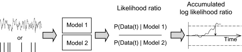
In the accumulated log-likelihood ratio (AccLLR) procedure, we detect selection time on each trial by measuring when an accumulating signal, a log-likelihood ratio, crosses a threshold (Wald 1975). Accumulation of sensory evidence in the form of log-likelihood ratios has been proposed as a mechanism by which the brain could discriminate between different sensory inputs (Gold and Shadlen 2007). According to this view, the level of firing in certain brain structures is hypothesized to reflect the current accumulated log-likelihood level. Here, we use log-likelihood ratios in a related but different way. We define log-likelihood ratios from neural activity and accumulate likelihood ratios to detect the timing of information in neural activity. We do this because using likelihood ratios allows us to use probabilistic models to transform point process measurements and continuous process measurements into a statistically equivalent representation. As we will show, after the neural signals are transformed into likelihood ratios, we can compute selection times from spiking and LFP activity using the same procedure.

Figure 1 illustrates the main components in the algorithm. We begin by defining two probabilistic models for the neural activity. These two models formally define the null and alternative hypotheses that we will select between when we compute the selection time. In the following we refer to these hypotheses as “condition 1” and “condition 2.” For a new trial of data, we calculate the log-likelihood ratio of the data, given the models, and accumulate the log-likelihood ratios over time. Selection time is defined as the time when the AccLLR crosses a threshold.

Fig. 1.

Schematic illustrating how spiking and local field potential (LFP) activity are processed to estimate selection time.

We now treat each stage of the algorithm in detail.

Probabilistic models of spiking and LFP activity

In this section, we present simple probabilistic models of spiking and LFP activity that we will use in the AccLLR framework. Using simple models allows us to derive simple expressions for the log-likelihood ratio and these simple expressions provide valuable insight that guides the development of the AccLLR procedure. The principal limitation of using simple models is the possibility that the models do not fit the data. When there is significant lack of fit between the models and the data, the resulting selection times will be misleading. The models we propose make Poisson and Gaussian distribution assumptions about the spiking and LFP activity, respectively. Although there are limitations of these models, analyses using Poisson and Gaussian assumptions are widely used in the literature and provide a useful starting point. We present statistics to assess the goodness-of-fit and present raw traces to assess the quality of the resulting selection times that demonstrate a good correspondence between the data and the results. More complex probabilistic models involving conditional dependence can also be applied within the AccLLR framework and may provide better fits to the experimental data and correspondingly more accurate selection times.

LFP model: Gaussian process model.

In the LFP model, LFP activity is modeled as independent observations from an underlying Gaussian distribution. The signal x(t) at time t is expressed as a mean waveform μ(t) with additive, Gaussian noise, ε(t)

$$x\left(t\right)=\mu \left(t\right)+\epsilon \left(t\right)$$ (1)

The likelihood of observed data x(t) being generated by each model is expressed as

$$P\left[x\left(t\right)-\mu \left(t\right)|{\sigma }^2\right]\sim N\left(0,{\sigma }^2\right)$$ (2)

The parameter space for the Gaussian process model of LFP activity is {Θ:μ(t), σ²}. The likelihood ratio for two time-varying Gaussian LFP models is expressed as

$$LL\left(t\right)=\log \frac{P\left[x\left(t\right)-{\mu }_1\left(t\right)|{\sigma }^2\right]}{P\left[x\left(t\right)-{\mu }_2\left(t\right)|{\sigma }^2\right]}=\frac{{\left(x\left(t\right)-{\mu }_2\left(t\right)\right)}^2-{\left(x\left(t\right)-{\mu }_1\left(t\right)\right)}^2}{2{\sigma }^2}$$ (3)

Note that in this expression, we set the noise in both models to have the same variance, σ². The difference between models is limited to the difference in the mean response profiles, μ(t). Extensions to allow changes in the variance of LFP activity and changes in the different frequency components in the power spectrum can also be considered.

Spiking model: inhomogeneous Poisson point process model.

In the spiking model, we model how many spike events occur at each interval in time N(Δt). Here, we assume that each spike event is independent of past spike events so that the spike time distribution follows a Poisson process with a time-varying firing rate, λ(t). Unlike the Gaussian model for LFP activity, there is no explicit noise term in the Poisson spiking model. Variability in the response emerges from the Poisson statistics of spike firing.

The likelihood of spiking activity at time bin Δt given the Poisson model is

$$P\left[N\left(\Delta t\right)|\lambda \left(t\right)\right]={\left(\lambda \left(t\right)\Delta t\right)}^{N\left(\Delta t\right)}\frac{\exp \left(-\lambda \left(t\right)\Delta t\right)}{N\left(\Delta t\right)!}$$ (4)

The log-likelihood ratio for two time-varying Poisson process spiking models is

$$LL\left(t\right)=\log \frac{P\left[\text{d}N\left(t\right)|{\lambda }_1\left(t\right)\right]}{P\left[\text{d}N\left(t\right)|{\lambda }_2\left(t\right)\right]}=\left({\lambda }_2\left(t\right)-{\lambda }_1\left(t\right)\right)\Delta t+\text{d}N\left(t\right)\log \left(\frac{{\lambda }_1\left(t\right)}{{\lambda }_2\left(t\right)}\right)$$ (5)

where dN(t) denotes the spike activity at each point in time N(Δt) and is equal to 0 or 1 for Δt = 1 ms. Formally, dN(Δt) = ∫_t^t+Δt dN(u). Like the LFP model, the difference between the models is limited to the response profiles, λ(t).

Accumulating the log-likelihood

The log-likelihood ratio LL(t) measures whether the evidence at time t for model 1 explains the observed neural activity better than model 2. Following the theoretical framework of discrete sequential probability ratio tests (Wald and Wolfowitz 1948), we decode whether model 1 or model 2 is represented in the observed data by integrating the evidence for model 1 compared with model 2 moment-by-moment from a start time t = 0 until a maximum accumulation time

$$\text{AccLLR}\left(t\right)={\displaystyle \sum _{t\prime =0}^t\text{LL}\left(t\prime \right)}$$ (6)

Accumulation is terminated in favor of model 1 when the AccLLR crosses the upper threshold. Accumulation is terminated in favor of model 2 when the AccLLR crosses the lower threshold. The selection time is defined as the time from the beginning of the accumulation to the time of threshold crossing. If neither threshold is crossed before the predetermined maximum time for accumulation, the selection time for the trial is unknown.

An important feature of the AccLLR procedure is that the observations can be point or continuous time series so we can apply the same AccLLR detection procedure to spiking and LFP activity. Moreover, the accumulated likelihood ratios follow a drift-diffusion process (Eckhoff et al. 2008). As a result, the individual statistical properties of spikes and fields are transformed to a representation where the same detection procedure can be applied to both signals.

Equation 3 shows how the accumulated log-likelihood ratio changes with each LFP observation x(t). The AccLLR changes by the relative distance, scaled by the noise variance, of the observation from the mean response for each condition. The AccLLR increases if the observation is closer to the mean response of condition 1 than to that of condition 2. The AccLLR decreases if the observation is closer to the mean response of condition 2 than that to condition 1.

Equation 5 shows how the AccLLR changes with each spike event. At each moment in time, the AccLLR increases by the difference in the firing rates for each model even when no spikes occur. In addition, if a spike occurs, dN(t) = 1, and the AccLLR discretely changes by the ratio of the model firing rates. If the spike occurs when λ₁(t) > λ₂(t), the spike supports model 1 and the AccLLR increases. If the spike occurs when λ₂(t) > λ₁(t), the spike supports model 2 and the AccLLR decreases.

Model fitting

For the Poisson model of spiking, we compute the firing rate λ(t), which quantifies the response of the single unit at a time t from an estimate of the time-varying firing rate. We estimated the firing rate by smoothing each spike event with a Gaussian, variance 5 ms, and averaging the activity across trials for each condition aligned to visual onset time.

For the Gaussian model of LFP activity, we estimate the mean response μ(t) by low-pass filtering the raw LFP activity at 40 Hz and averaging the activity across trials for each condition aligned to onset time. We estimate the noise variance separately for each condition by subtracting the fitted mean response μ(t) from the raw traces and calculating the total variance of the residuals. We combine the estimates of the noise variance for each condition into a single estimate of noise variance by averaging the variances. This is equivalent to estimating the variance by pooling the data from both conditions. Since AccLLR changes for LFP activity are scaled by the noise variance for each condition, if the noise variances for each condition differ, the AccLLRs scale differently and this leads to the need for different upper and lower bounds at the discrimination stage. To allow the simplicity of using the same bound for both conditions (see the following subsection), we assume that the variance of activity under each condition is the same. Future work can consider the case of asymmetric bounds.

Setting the detection threshold level

The level of the detection threshold drives the performance of the detection procedure and is a central issue in the AccLLR method. We depart from the theory underlying discrete sequential probability ratio tests laid out by Wolfowitz and Wald (1948) because we set the level for the threshold crossing empirically (see results). We measure performance in terms of the correct detect probability, the false alarm probability, and the mean correct detect selection time. The correct detect probability is given by the proportion of trials from condition 1 whose AccLLR hit the upper detection threshold within the maximum accumulation time. The false alarm probability was estimated by the proportion of trials from condition 2 whose AccLLR hit the upper detection threshold within the maximum accumulation time. The correct detect selection time was estimated as the average selection time for the correctly classified trials from condition 1. Varying the threshold level significantly changes the trade-off between correct detection, false alarm rate, and selection time.

We define selection time curves (see Fig. 3 for an example) by varying the level of the detection threshold from a very low level, 0.5% of the maximum AccLLR, to the maximum AccLLR. We elected to terminate accumulation at 200 ms. This time was considered to be the latest time that neural signals reflect visual onset, which is the application on which we focus here. We could choose to terminate accumulation at longer or shorter times. The correct detect selection time curve is defined by varying the detection threshold and measuring the correct detect probability and the correct detect selection time. The false alarm selection time curve is similarly defined by varying the detection threshold and measuring the false alarm probability and the correct detect selection time. The selection time curves reveal how changing the level of the detection threshold influences performance measures. We use the selection time curves to select levels with the same false alarm performance to make appropriate comparisons about correct detect and selection time performance between different signals and different methods.

Fig. 3.

Spike example single trial analysis. A: probability of correctly detecting a single trial from condition 1, “hit” (solid). Probability of incorrectly classifying a condition 1 trial as being from condition 2, “false reject” (dashed). Probability of not classifying a condition 1 trial, “don't know” (dotted). Each probability is plotted as the level of the AccLLR detection threshold is varied from a low value to a maximum value. B: probability of correctly rejecting a single trial from condition 1 and assigning it to condition 2, “reject” (solid). Probability of incorrectly classifying a condition 2 trial as being from condition 1, “false alarm” (dashed). Probability of not classifying a null condition trial, “don't know” (dotted). Each probability is plotted as the threshold level is varied. C: mean selection time for correctly detected, “hit,” condition 1 trials as the threshold is varied. D: probability of correctly detecting a single trial from condition 1, “spike hit” plotted against the selection time as the level of the detection threshold is varied (circle). Probability for incorrectly detecting a trial from condition 2, “spike false alarm” (square). E: rasters of condition 1 spike activity for correctly detected trials (black). Rasters are sorted by selection time. Selection time calculated for each trial is marked (black rectangle). Rasters of condition 1 spike activity for missed and incorrectly detected trials (gray). F: average firing rate for correctly detected condition 1 trials aligned to selection time; 95% CI (shaded).

Controlling signal quality

When comparing selection times for two different neural signals, selectivity may emerge in one signal before the other signal, but eventually both signals could have the same selectivity. If so, differences in selection times result from a difference in when each signal became selective for the task. However, differences in signal selectivity can bias estimates of selection time. If one signal is significantly more selective than the other, a difference in selection times could simply result from a difference in when we can detect selectivity and may not result from a difference in the timing of the underlying activity.

We would like to compare selection times between different neural signals without being biased by the selectivity of each signal. This should be possible if we could match signal selectivity. One approach to matching signal selectivity is to match neural signals by artificially increasing the variability in the signal that is more selective. The idea is to reduce the selectivity of the more selective signal to match the less selective signal. We define signal selectivity with the choice probability from a receiver-operating characteristic (ROC) analysis of the AccLLR traces.

Gaussian case.

We increase the variability of LFP signals by adding uncorrelated Gaussian noise to the activity at each time step. This procedure does not alter the mean firing rate for each condition, but reduces the overall selectivity. We vary the SD of the added Gaussian noise so that the performance of an ideal observer decoding the AccLLR at the end of the temporal integration interval is the same for the two signals we were comparing. We characterize the performance of an ideal observer using the choice probability of an ROC analysis.

Poisson case.

We reduce the selectivity of spiking signals without changing the mean responses by adding and deleting spikes from individual trials in a manner that increases the trial-to-trial variability in the spike count and preserves the average number of spikes at each time. We use the fact that increasing the number of doublets in a spike train increases the trial-to-trial variability of spike counts, the Fano factor (Daley and Vere-Jones 2002), and define a probability of deleting spikes from each trial and adding the spike precisely 2 ms after a spike in another a trial. Specifically:

1. For each 5 ms time interval, enumerate all the trials with at least one spike.

2. Delete a spike from each trial in the 5 ms interval with probability P.

3. For each deleted spike, find a remaining spike that is followed by a quiet period of 3 ms and add a spike 2 ms after it.

Since we do not change the number of spikes at each 5-ms interval, we do not change the mean firing rate of the activity. However, since the reassigned spikes tend to come in doublets and not individually, the trial-to-trial variability in spike counts increases. We vary the probability of moving spikes (P) so that the performance of an ideal observer decoding the AccLLR at the end of the temporal integration interval is the same for the two signals. We characterize the performance of an ideal observer using the choice probability of an ROC analysis.

ROC analysis

We performed an ROC analysis on the AccLLR values to quantify signal selectivity. Analysis was performed every millisecond to discriminate activity from condition 1 and condition 2 trials. Overall signal selectivity was defined as the choice probability from the ROC analysis at the end of a 200-ms accumulation interval.

Trial-average selection time

In addition to computing selection times from activity on a single trial, we compute selection times for an average of multiple trials. We do this by assuming that activity on each trial is independent of activity on any other trial. The trial-average log-likelihood ratio is then the sum of the log-likelihood ratio of activity on each trial

$${\text{LLR}}^{\text{trial}}\left(t\right)={\displaystyle \sum _{i=0}^N{\text{LL}}^{\left(i\right)}\left(t\right)}$$

where N is the number of trials in the trial average and i indexes the single-trial log-likelihood ratios. The selection time for the trial-average response is computed from the AccLLR in the same way as the single-trial selection time, that is, by measuring the correct detect and false alarm probabilities while varying the level of detection threshold. We constructed 95% confidence intervals (CIs) for the mean selection times at each trial average using a bootstrap procedure (Efron and Tibshirani 1994).

Overfitting can be especially pronounced when decoding trial average quantities and is revealed by unreasonably early selection times, such as 0 ms, together with unreasonably high correct detect probabilities and low false alarm probabilities. To avoid overfitting, we partitioned the data set into a training set and a test set. Models were fit using trials only in the training set. Trial-average AccLLRs were computed using groups of trials drawn from the test set. When trial-averaging we use a leave-N-out procedure. For example, if we intend to test averages of N trials, we define a training set using all the trials except for N trials and fit the models using only these trials. We then define a test set of N trials that we use to calculate the log-likelihood ratio.

Experimental procedures

Experimental data in this study were collected from one adult male rhesus macaque. All surgical and animal care procedures were done in accordance with the National Institute of Health guidelines and were approved by the New York University Animal Care and Use Committee.

Behavioral task.

Behavior was controlled using custom LabVIEW (National Instruments, Austin, TX) code running on a real-time PXI platform. Eye position was monitored with an optical video eye tracker (ISCAN, Cambridge, MA). A light-emitting diode stimulus board or liquid crystal display was placed behind a glass touch screen oriented in a vertical plane in front of the monkey so that eye and arm movements were made in the same visual workspace. Each trial was initiated when the monkey touched a pair of proximity sensors placed near the body with his hands. The nonreaching hand was required to maintain touch on a proximity sensor throughout the trial. Access to water was controlled during training and testing and the animal was habituated to head restraint and trained to perform behavioral tasks for a liquid reward. A brief auditory tone preceding reward delivery served as a secondary reinforcer on all correct trials.

The monkey performed a memory-guided saccade task involving a saccade from a central location to a peripheral target. The trial started with the illumination of a central red and green stimulus. The monkey fixated and touched the central target location and waited 500–800 ms. Subsequently, a peripheral red target was flashed for 100 ms, followed by a delay of 1,000–1,500 ms. The monkey was then cued through extinction of the central red fixation target to saccade to the remembered position of the red target. The monkey waited until the go signal for each movement before promptly making that movement. He had to respond to the go signal with a saccade within 350 ms. To keep monkeys from trying to predict the go signal, trials were aborted if the saccade reaction time was <100 ms. After holding the target successfully for 300–500 ms, the monkey was given a liquid reward.

Data collection and preprocessing.

Eye position and touch position on the screen were sampled at 1 kHz. Each signal was time-stamped and streamed to disk along with data about each trial from the LabVIEW behavioral control program. The time of cue presentation was recorded as the time at which a photosensor detected a simultaneous stimulus change on the monitor. Spiking and LFP activity were recorded with 1 MΩ tungsten electrodes (Alpha Omega, Nazareth Illit, Israel). Neural signals were amplified (×10,000; TDT Electronics, Alachua, FL), digitized at 20 kHz (National Instruments), and continuously streamed to disk during the experiment (custom C and Matlab code). LFP activity was generated by low-pass filtering the raw, broad-band recording at 300 Hz and decimating the signal to 1 kHz. Single-unit activity was generated by band-pass filtering the signal from 0.3 to 6.6 kHz, extracting waveforms that crossed a threshold (typically 3.5 SDs of the band-pass filtered activity), upsampling and aligning waveforms to the peak negativity or positivity, and semiautomatically clustering waveforms on a 100-s moving-window. Typically, spike clusters were overclustered automatically and then clusters were manually inspected and merged.

RESULTS

We develop the AccLLR procedure for computing selection times using a set of example recordings of spiking and LFP activity in the posterior parietal cortex (PPC) of a monkey performing a memory-guided saccade task. We first present the computation of selection time using an example spike recording and an example field recording. We then illustrate the issues in using the technique with three examples of simultaneous spike-field recordings, comparing the selection times on average and trial by trial. Finally, we illustrate the influence of controlling signal selectivity on selection times computed from spiking and LFP activity.

Likelihood ratios for spiking and LFP activity

We use an example recording of spiking activity during a memory-guided saccade task to develop the AccLLR procedure for computing selection times. In this task, a visual target flashed at a peripheral location directs a remembered saccade. Spiking and LFP activity in the PPC are known to encode the location of the visual stimulus. At what time after the visual stimulus is illuminated does neural activity become selective for the visual stimulus, known as the visual onset time?

To compute the visual onset time using the likelihood procedure, we need to define two models. The choice of these two models defines the nature of the information processing that underlies the selection time. For visual onset, we define model 1 using activity recorded for 200 ms immediately following the onset of the visual stimulus (condition 1). We define model 2 using activity during a 200-ms baseline period involving stable fixation but no visual stimulation (condition 2). We assess the likelihood of the data under each model and accumulate the log-likelihood ratio in time until there is sufficient evidence in support of either model. If sufficient evidence is not obtained in support of either model by 200 ms, we declare the trial as “don't know.”

Figure 2A shows the mean firing rate response of a neuron averaged across trials for condition 1 (solid) and condition 2 (dashed). Calculating the AccLLR from spiking for each trial drawn from condition 1 reveals a tendency for the AccLLR to increase after a certain time (Fig. 2, B and D). Conversely, the AccLLR tends to decrease for trials drawn from condition 2 (Fig. 2, C and D). Sample AccLLR traces highlighted in black illustrate the low firing rate spiking activity from condition 2. The AccLLR contains few discrete jumps and the path is dominated by the difference in mean firing rate. In contrast, activity from condition 1 has a series of steps given by the arrival times of each spike. Computing the trial-average AccLLR for each signal more clearly shows the tendency for the AccLLR to increase for condition 1 and decrease for condition 2 (Fig. 2D). We also performed ROC analysis at each moment in time to discriminate the AccLLR for condition 1 compared with condition 2 and provide an overall measure of signal selectivity (Fig. 2E).

Fig. 2.

Example spike recording. A: firing rate for condition 1 (solid) and condition 2 (dashed). Rasters of spike activity during condition 1 (black) and condition 2 (gray). B: accumulated log-likelihood ratio (AccLLR) between conditions 1 and 2 for each trial during event condition. Sample trace highlighted for clarity (black). C: AccLLR for each trial during condition 1. Sample trace (black). D: mean AccLLR for trials during condition 1 (solid) and condition 2 (dashed). E: choice probability from receiver-operating characteristic (ROC) analysis applied to AccLLR traces at each time bin following onset for event condition and null condition; 95% confidence intervals (CIs) (shaded).

Single-trial spike selection times

To compute selection times from single trials, we applied a pair of thresholds to the AccLLR at an equal distance above and below the null line, AccLLR = 0. Activity that did not hit either threshold within 200 ms was classified as a “don't know” error and no selection time was computed.

Instead of setting a single threshold, we characterize performance and selection times for correct detects as we vary the level of the threshold. This is in the spirit of the ideal observer analysis performed in ROC analyses. The main differences are that in this situation three classifications are possible for each trial—hits, false alarms, and don't knows—and we relate performance to selection times.

As we increase the level of the detection thresholds from AccLLR = 0, a trade-off takes place between the speed (selection time) and accuracy (probability correct classification; Fig. 3, A–C). At very low levels, selection times are very fast but performance is very poor. As the level is raised from low levels, selection time increases, the probability of a hit increases, and the probability of a false alarm decreases. The trade-off changes when the level is increased further. Selection time continues to increase with increasing level, although performance begins to decline. This is because when the level of the detection threshold becomes too high, increasingly more trials are classified as “don't know.” Simultaneously, hits and false alarms both decrease. At the limit of a very high level, the probability of a hit or a false alarm becomes zero.

Figure 3D plots the selection time curves for single trials from the example spike recording. Each point shows the performance, either hit or false alarm, and the average selection time for a particular level of the detection threshold. The best overall hit performance for spiking activity was 82%, with a mean hit selection time of 112 ms. At this detection threshold, the false alarm rate was 12%. Rasters from individual trials (Fig. 3E) show that correctly detected trials were associated with increased firing immediately before selection. Interestingly, rasters from the missed trials did not contain any increased activity, suggesting that when activity is robust, as in this example, variability in detection comes from intrinsic variability in the response. These results demonstrate that the AccLLR procedure can reliably estimate selection times from spiking activity in single trials.

Trial-average spike selection times

We were also interested in how long after the increase in firing selection was detected, which we call the detection lag. Examination of the rasters showed that the lag in detection was on the order of several spikes. Calculating the average firing rate of activity aligned to selection showed an increase in firing <10 ms before detection (Fig. 3F). We reasoned that the detection lag should be smallest when computing selection times by averaging activity across many trials because the signal to noise ratio should be greater compared with activity from single trials. If so, the detection lag should be reflected in a decrease in the mean selection time decreases as we averaged activity from more trials.

To test this, we compared selection times using the AccLLR procedure after combining log-likelihood ratios for 1, 2, 5, 10, 15, 20, and 25 trials (Fig. 4). Increasing the number of trials in the trial average clearly improved performance, producing 100% detection when averaging as few as 5 trials (Fig. 4B). However, although selection times with the 100% hit performance became smaller as the number of trials in the average increased (Fig. 4D, dashed) the probability of false alarm also dramatically increased (Fig. 4C, dashed).

Fig. 4.

Spike example trial average analysis. A: probability of correctly detecting activity from one trial or from an average of 2, 5, 10, 15, 20, and 25 trials from condition 1, “spike hit” plotted against the selection time as the level of the AccLLR detection threshold level is varied from a low value to a maximum value (circle, dot). Probability for incorrectly detecting a trial from condition 2, “spike false alarm” (square, cross). Numbers within the panel denote number of trials in the average. B: probability of correctly detecting condition 1 activity as the number of trials in the average is varied. C: probability of a false alarm, detecting condition 2 activity, as the number of trials in the average is varied. D: mean selection time for correctly detected condition 1 trials as the number of trials in the average is varied. B–D: results when threshold detection level is set to give the greatest correct probability and fastest selection time when the false alarm probability is set to 0 (solid). Results when the threshold detection level is set to give the greatest correct probability (dashed).

The reduction in selection time as the false alarm rate increases illustrates a problem in comparing selection times. Speed can be traded-off against accuracy, in this case false alarm accuracy. Therefore when making comparisons, we need to control the false alarm rate. When we selected the level of the detection threshold to give a constant false alarm probability equal to 0 (Fig. 4C, solid), we found the selection times decayed more gradually. Selection times fell from 115 ms when using a single trial to <100 ms when averaging ≥15 trials (Fig. 4D, solid). The trial-average analysis indicates that, for this example, the detection lag when analyzing single trials is about 15 ms.

Example LFP recording

We applied the same analysis methodology to an example LFP recording. LFP activity in the event condition revealed a strong, selective response (Fig. 5A). AccLLR traces increased for condition 1 and decreased for condition 2. Unlike the traces from spiking activity, the AccLLR traces from LFP activity changed smoothly with time (Fig. 5, B and C, black). The average AccLLR trace showed a steady increase following the onset (Fig. 5D), albeit with a noticeable flattening when the mean waveforms for conditions 1 and 2 crossed at around 150 ms after visual stimulus onset (Fig. 5A), as predicted by Eq. 3. The ROC analysis showed that the example LFP activity became strongly selective about 200 ms after visual stimulus onset (Fig. 5E).

Fig. 5.

Example LFP recording. A: mean LFP response for condition 1 (solid) and condition 2 (dashed). B: AccLLR between conditions 1 and 2 for each trial during condition 1. Sample trace highlighted for clarity (black). C: AccLLR for each trial during condition 2. Sample trace (black). D: mean AccLLR for trials during condition 1 (solid) and condition 2 (dashed). E: choice probability from ROC analysis applied to AccLLR traces at each time bin following onset for conditions 1 and 2. 95% CIs (shaded).

The best correct detect performance decoding single trials of LFP activity is 75%, with an 11% false alarm rate (Fig. 6A). The mean selection time at this false alarm rate is 136 ms. Except for a small minority of trials, selection times are detected at the peak negativity of the LFP waveform and a shift in the time of the negativity can be observed with selection time on each trial (Fig. 6B). Aligning the waveforms to the selection times and averaging across correctly detected trials suggest that, unlike in the spiking example, detection of selection times lagged the initial positive deflection by as much as 50 ms (Fig. 6C). The trial-average data support this (Fig. 7). When the false alarm probability is set to 0, selection times decrease from 156 ms for single trials to 121 ms when averaging 25 trials (Fig. 7D).

Fig. 6.

Example LFP recording single trial analysis. A: probability of correctly detecting a single trial from condition 1, “LFP hit” plotted against the selection time as the level of the AccLLR detection threshold is varied from a low value to a maximum value (circle). Probability for incorrectly detecting a trial from condition 2, “LFP false alarm” (square). B: waveforms of condition 1 LFP activity color-coded on a linear scale. Waveforms are sorted by selection time. Selection time calculated for each trial is marked (black rectangle). Waveforms of condition 1 LFP activity for missed and incorrectly detected trials are plotted above. C: mean LFP response for correctly detected condition 1 trials aligned to selection time; 95% CIs (shaded).

Fig. 7.

Example LFP recording trial average analysis. A: probability of correctly detecting activity from one trial or from an average of 2, 5, 10, 15, 20, and 25 trials from the event condition 1, “LFP hit” plotted against the selection time as the level of the AccLLR detection threshold level is varied from a low value to a maximum value (circle, dot). Probability for incorrectly detecting a trial from condition 2, “LFP false alarm” (square, cross). Numbers within the panel denote number of trials in the average. B: probability of correctly detecting condition 1 activity as the number of trials in the average is varied. C: probability of a false alarm, detecting condition 2 activity, as the number of trials in the average is varied. D: mean selection time for correctly detected condition 1 trials as the number of trials in the average is varied. B–D: results when threshold detection level is set to give the greatest correct probability and fastest selection time when the false alarm probability is set to 0 (solid). Results when the threshold detection level is set to give the greatest correct probability (dashed).

The results for both spiking and LFP activity show that the position of the detection threshold drives performance and defines a trade-off between detection speed and accuracy. Interestingly, we observe that when we enforce good accuracy, detection lags the changes visible in the raw traces. Trial-averaging reduces the lag and a comparison of how the lag stabilizes as the number of trials in the average increases provides a way to assess the earliest time that a signal is present in a given recording.

Simultaneously recorded spike-field examples

We now present three examples of simultaneously recorded spike-field sessions to illustrate how the AccLLR procedure handles different types of recordings. Spiking and LFP activity from the first example are presented as in the preceding example recordings (Figs. 2–7) and plotted for direct comparison in Fig. 8. The choice probability from the ROC analyses shows that spiking and LFP activity in this recording contain the same amount of information about the onset of the visual stimulus but that spiking becomes significantly selective earlier than LFP activity (Fig. 8A). The selection time curves from individual trials are consistent with this result (Fig. 8B). When we control the detection threshold level to equalize the false alarm rates to 0.05, the mean spike selection time is 129 ms, with a hit probability of 0.79. The mean LFP selection time is 147 ms, with a hit probability of 0.78.

Fig. 8.

Example simultaneous spike and field recording 1. A: choice probability from ROC analysis applied to LFP (solid) and spike (dashed) AccLLR traces at each time bin following onset for conditions 1 and 2. B: single trial selection time curve for correct detection of spiking (circle), false alarm detection of spiking (square), correct detection of LFP activity (dot), and false alarm detection of LFP activity (cross); 95% CIs (shaded). Spiking activity same as example recording in Figs. 2–4. LFP activity same as example recording in Figs. 5–7.

LFP activity is not always selective later than the spiking activity of this neuron. In the second spike-field example (Fig. 9), we compare spiking activity from the neuron in Fig. 8 (shown here in Fig. 9A) with LFP activity from another site. Mean LFP response waveforms are significantly different, with a less pronounced positive rise in the event condition trials (Fig. 9B). ROC analyses reveal that spike and LFP activity have similar timing and overall selectivity (Fig. 9C). Analyzing the single-trial selection time curves reveals slight differences. The best LFP selection time is 112 ms, with a hit probability of 0.8 and a false alarm probability of 0.09. The best spike selection time is 122 ms, with a hit probability of 0.88 and a false alarm probability of 0.09. When the false alarm probability is controlled to 0.05, LFP selection time increases to 117 ms, with hit probability of 0.69, and spike selection time increases to 129 ms, with a hit probability of 0.83. The single-trial selection time estimates from spiking and LFP signals follow the variability in the activity (Fig. 9, E and F). Selection time is earlier on trials with correspondingly earlier changes in activity. Analysis of LFP waveforms aligned to the selection time shows that the earlier LFP detection in this recording may result from the lack of an initial rise before the dip in the mean waveform, which reduces the lag in selection time detection (Fig. 9H).

Fig. 9.

Example simultaneous spike and field recording 2. A: firing rate for condition 1 (solid) and condition 2 (dashed). B: mean LFP response for condition 1 (solid) and condition 2 (dashed). C: choice probability from ROC analysis applied to LFP (solid) and spike (dashed) AccLLR traces at each time bin following onset for conditions 1 and 2. D: single trial selection time curve for correct detection, hit, of spiking (circle), false alarm detection of spiking (square), correct detection of LFP activity (dot), and false alarm detection of LFP activity (cross). E: rasters of condition 1 spike activity for correctly detected trials (black). Rasters are sorted by selection time. Selection time calculated for each trial is marked (black rectangle). Rasters of condition 1 spike activity for missed and incorrectly detected trials (gray). F: waveforms of condition 1 LFP activity color-coded on a linear scale. Waveforms are sorted by selection time. Selection time calculated for each trial is marked (black rectangle). Waveforms of condition 1 LFP activity for missed and incorrectly detected trials are plotted above. G: average firing rate for correctly detected condition 1 trials aligned to selection time. H: mean LFP response for correctly detected condition 1 trials aligned to selection time; 95% CIs (shaded). Spiking activity recorded from same cell as spike-field example 1 in Fig. 8. LFP activity is from an electrode different from that of the example spike and field recording 1.

The third spike-field example features activity from a different neuron and LFP site. Spiking responds briskly but somewhat transiently following the onset of the visual stimulus (Fig. 10A). Average LFP activity responds with an initial dip followed by a pronounced rise (Fig. 10B). ROC analyses show that LFP activity is more selective and emerges sooner than spiking, although the increase in LFP selectivity emerges somewhat slowly (Fig. 10C). The single-trial selection time curves support this analysis (Fig. 10D). Although the spike hit probability peaks before the LFP hit probability, when the detection level is set to control the false alarm rate to 0.05, the selection times are more nearly equal. LFP selection times are 145 ms, with a hit probability of 0.85, and spiking selection times are 138 ms, with a hit probability of 0.61. The selection time aligned mean spiking rates and rasters show that the lag in selection time detection is relatively short, <10 ms (Fig. 10, E and G). In contrast, LFP activity has a longer detection lag of around 35 ms (Fig. 10, F and H).

Fig. 10.

Example simultaneous spike and field recording 3. A: firing rate for condition 1 (solid) and condition 2 (dashed). B: mean LFP response for condition 1 (solid) and condition 2 (dashed). C: choice probability from ROC analysis applied to LFP (solid) and spike (dashed) AccLLR traces at each time bin following onset for conditions 1 and 2. D: single trial selection time curve for correct detection of spiking (circle), false alarm detection of spiking (square), correct detection of LFP activity (dot), and false alarm detection of LFP activity (cross). E: rasters of condition 1 spike activity for correctly detected trials (black). Rasters are sorted by selection time. Selection time calculated for each trial is marked (black rectangle). Rasters of condition 1 spike activity for missed and incorrectly detected trials (gray). F: waveforms of condition 1 LFP activity color-coded on a linear scale. Waveforms are sorted by selection time. Selection time calculated for each trial is marked (black rectangle). Waveforms of condition 1 LFP activity for missed and incorrectly detected trials are plotted above. G: average firing rate for correctly detected condition 1 trials aligned to selection time. H: mean LFP response for correctly detected condition 1 trials aligned to selection time; 95% CIs (shaded).

The example recordings demonstrate that the AccLLR method can accurately track changes in spiking and LFP activity on single trials. Selection times and the accuracy of the method on individual trials depend on the timing and strength of the signal on each trial.

Testing goodness of fit

We analyzed the two example spike recordings and three example LFP recordings to test the goodness of fit of the models for each condition (Fig. 11). We tested the goodness-of-fit of the spike recordings using a Kolmogorov–Smirnov (K-S) test applied to the distribution of interspike intervals (ISIs) after rescaling by the fitted conditional intensity function. The time rescaling theorem (Brown et al. 1998) states that any point process with an integrable rate function may be rescaled to a Poisson process with unit rate. The goodness of fit for the first example spike recording (from Figs. 2–4, 8, and 9) revealed departures of the rescaled ISIs from Poisson during condition 1 and condition 2 (Fig. 11A). The degree of lack of fit during condition 1 was moderate but significant (P < 0.05, K-S test). Lack of fit of data from condition 2 was also significant (P < 0.05, K-S test). The second example spike recording (from Fig. 10) also revealed lack of fit during both conditions (P < 0.05, K-S test; Fig. 11B). However, in each case, we did not observe gross departures from the Poisson spiking model. These results indicate that although the Poisson spiking model does not fully account for spiking activity, it is effective at detecting selection times in the data consistent with performance of the selection times on the raw spike rasters in Figs. 3, 9, and 10.

Fig. 11.

Model goodness-of-fit. A: goodness-of-fit for example spike recording 1 for activity during conditions 1 (left) and 2 (right). The empirical cumulative distribution function (CDF) of the interspike intervals (ISIs) is plotted against the sample CDF of the ISIs after rescaling time according to the fitted condition intensity function (solid). The CDF for a uniform distribution (dashed); 95% CI (dotted). B: same as A for example spike recording 2. C: goodness-of-fit for example LFP recording 1 during conditions 1 (left) and 2 (right). Quantile–quantile (Q-Q) plot for the residuals of LFP activity after the fitted mean response has been subtracted. Samples from LFP activity (dots). Gaussian distribution (dashed); 95% CI (dotted). D: same as C for example LFP recording 2. E: same as C for example LFP recording 3.

We examined the goodness of fit of the example LFP recordings using quantile–quantile (Q-Q) plots plotting the residual activity after subtracting the model fits against a standard Gaussian distribution. We tested the goodness of fit of the LFP recordings using a K-S test. Q-Q plots of all three example recordings during both conditions revealed that the residuals were distributed according to a Gaussian, except for the tails of the distributions (Fig. 11, C–E). LFP activity for all three example recordings was not significantly non-Gaussian (example 1: condition 1, P = 0.59, condition 2, P = 0.16; example 2: condition 1, P = 0.67, condition 2, P = 0.22; example 3: condition 1, P = 0.09, condition 2, P = 0.70; K-S test).

Thus Poisson and Gaussian models can provide reasonably good fits to the spiking and LFP activity during visual stimulation. Improvements in model fits will further improve performance of the AccLLR method.

Comparing selection times computed from spiking and LFP activity

The preceding sections demonstrate that the AccLLR framework provides a systematic procedure for analyzing the timing of information processing in spiking and LFP activity on individual trials and averaged across multiple trials. Calculating selection time allows us to examine the relative timing of information in spiking and LFP activity on average and how timing covaries across trials. The single-trial selection time curves in Figs. 8–10 address whether information in spiking precedes or follows LFP activity. However, conclusions drawn from single trials are confounded by differences in the selection time detection lag. Calculating how selection times differ on average is best done by comparing selection times computed from multiple trials instead of single trials because the detection lag is reduced by combining information present across many trials.

Figure 12, A–C compares timing between spiking and LFP activity when we minimize the detection lag by plotting how selection times vary as the number of trials in the average increases. The best selection times for the first spike-field recording are 127 ms for LFP and 107 ms for spiking. For the second spike-field recording, the best LFP selection time is 95 ms and the best spike selection time is 108 ms. For the third spike-field recording, the best LFP selection time is 105 ms and the best spike selection time is 128 ms. In each case, the false alarm rate is set to 0 and the hit probability quickly increases to 1 for spiking and LFP activity. These results show how the AccLLR framework can be used to compare average selection times for different signals. In each case, selection times initially fall and then stabilize as the number of trials in the trial average increases. Stabilization indicates detection lag is minimized when averaging large numbers of trials. The results also suggest that a minimum time can be defined. Before this time, neural signals do not contain information about the visual stimulus onset on average.

Fig. 12.

Comparison of spike and LFP activity in example spike and field recordings. A–C: mean selection time for spike (dashed) and LFP (solid) activity as number of trials in the average is varied from 1 to 25 trials. Results are shown when threshold detection level is set to give the greatest correct probability and fastest selection time and the false alarm probability is controlled to be 0. D–F: correlations between single trial selection times from simultaneously recorded spike activity and LFP activity for all correctly detected condition 1 trials. Spike-field selection times for each trial are shown by a cross. Spearman's rank correlation coefficient is shown in each panel. A and D: example spike and field recording 1. B and E: example spike and field recording 2. C and F: example spike and field recording 3.

Understanding how selection times covary between spiking and LFP activity involves successfully computing selection times from single trials and then analyzing the covariations. Since we are interested in covariations and not average durations, we do not need to minimize the detection lag as long as we can assume that the detection lag is consistent across trials. Figure 12, D–F presents trial-by-trial covariations in selection times for each spike-field example. The first and second spike-field recordings have no significant correlation in selection times [first recording: r = 0.22 (Spearman's rank-correlation coefficient), P = 0.15 (permutation test); second recording: r = 0.11, P = 0.45]. However, the third spike-field recording contains strong evidence of covariation between spiking and LFP selection times across single trials (r = 0.41, P < 0.01). Therefore the method is sufficiently sensitive to detect covariation despite the detection lag.

Although computing selection times from single trials can be influenced by a lag in detection, the AccLLR method can reliably detect covariations in single-trial selection times. When making comparisons between the mean selection times from different recordings, the detection lag can be minimized by averaging trials and observing selection times stabilize.

Matching signal selectivity

Finally, we address the problem of comparing selection times between signals with different degrees of selectivity. The selection time curves (see preceding text) show that selection time is influenced by a trade-off between speed and accuracy. We can control this trade-off for different estimates of selection time by constraining the false alarm probability of the detection procedure. It is possible that estimates of selection time are also biased by another factor, the overall selectivity of the signal. More selective signals with larger changes in activity can give shorter detection lags. To control for differences in signal selectivity, we need to match the amount of selectivity in different signals. Note that this concern need not preclude the possibility that response magnitude and latency are genuinely correlated (Maunsell and Gibson 1992). However, the possibility that latency estimates can be biased by changes in response magnitude merits attention.

One way to match signal selectivity is to reduce the selectivity of the more selective signal. In methods, we presented procedures to reduce signal selectivity for spiking and LFP activity, which involve artificially increasing the variability of the signal. These procedures do not alter the mean responses to each trial condition but progressively increase the amount of variability, thus reducing the signal to noise. Here we test whether we can successfully control the degree of signal selectivity using these procedures.

Figure 13 presents the results of applying each procedure to activity from the third example spike-field recording. Increasing spiking noise reduces signal selectivity, reduces the hit probability, and increases the selection time (Fig. 13, A–C). The same pattern of results is observed when adding noise to LFP activity (Fig. 13, D–F).

Fig. 13.

Performance as signal selectivity is matched in third spike and field example recording from Fig. 10. A: spike choice probability from ROC analysis of AccLLR traces as spike noise, probability of doublet bursts, increases. B: spike correct detection probability from single trial decoding as the spike noise increases. At each noise level, the level of the detection threshold is set to a false alarm probability of 0.05. C: spike mean selection time for correctly detected condition 1 trials as probability of spike noise is increased. D: LFP choice probability from ROC analysis of AccLLR traces as the variance of added Gaussian noise is increased. E: LFP correct detection probability from single trial decoding as the LFP noise increases. False alarm probability is set to 0.05. F: LFP mean selection time for correctly detected condition 1 trials as LFP noise is increased.

These results show that we can control signal selectivity and that lower selectivity leads to increased selection times. Therefore we can use the AccLLR framework to make meaningful comparisons between selection times, even when signals have different amounts of selectivity by matching signal selectivity.

DISCUSSION

We have presented a method for estimating selection times in neural activity that is designed to satisfy three criteria: 1) selection times should be computed on individual trials; 2) they should be computed from both spiking and LFP activity; and 3) they should allow us to make comparisons between different recordings. Our approach defines selection time as the time that an observer can use observations of neural activity to distinguish between two hypotheses. Each hypothesis involves a set of trial conditions and neural activity recorded under those conditions is used to fit the parameters of a probabilistic model. Selection occurs when the accumulated log-likelihood ratio between the models crosses a threshold.

The first criterion, single trial detection, requires that the method be sensitive and reliable. Unlike reports of excessive variance in the latency of single trial detection methods, we see that the AccLLR method seems to track the degree of variability present in the underlying neural activity. The second criterion, applicability to spiking and LFP activity, is satisfied by transforming raw neural observations, with statistical properties, into the likelihood ratio domain in which the observations behave as a drift-diffusion process (Eckhoff et al. 2008). After transformation into likelihood ratios, we use the same detection procedure for both spiking and LFP observations. The third criterion, permitting comparisons, is satisfied by setting the threshold to explicitly control the performance of the detector and by matching signal selectivity. Applications of the method to experimental data illustrate each point.

Analyzing the timing of information in neural activity

There are serial and parallel routes for information to travel through the nervous system. In the visual system, these routes have been placed in the context of a hierarchy of regions extending from the retina through primary visual cortex up through the dorsal and ventral visual streams (Felleman and Van Essen 1991). In general, however, the functional properties of neural activity do not satisfy simple models of distributed information processing. Comparisons of the average time when information is present in neural activity have found that multiple cortical areas are active at the same time and that the activity in these areas can encode similar functional responses (Bullier and Nowak 1995).

A promising way to disentangle the organization of distributed brain processes is to perform recordings and causal manipulations simultaneously across multiple brain regions and to measure covariations in the timing of neuronal responses instead of the average response times. Although experimental techniques to monitor multiple brain regions are progressing rapidly (Buzsáki 2004), progress toward resolving how information propagates between brain regions has been hampered by technical limitations in reliably measuring the timing of activity on single trials. The main limitation is that measures of timing on single trials have been unreliable, precluding the effective study of covariations in timing. The AccLLR method presented here aims to overcome current limitations in analyzing signal timing to facilitate the examination of distributed processing. Our results demonstrate that the AccLLR method can measure selection times on single trials and so can be an effective tool in the analysis of a range of neural signals encompassing both spiking activity and LFP activity.

Alternative formulations of selection time using AccLLR

A strength of the AccLLR method is the diversity of alternative formulations it allows. In this study, we have used selection time defined by stimulus onset detection: the time when neural activity contains information about the presence or absence of a stimulus. Many alternative selection times can be defined and analyzed. For example, selection times can be given by the time when one stimulus can be discriminated from another stimulus, when an action will be selected or when an action will be canceled (Hanes et al. 1998; Hung et al. 2005; Thomas and Paré, 2007). Comparisons between selection times defined by different hypotheses are then possible and offer the potential to track transformations across circuits (Monosov et al. 2008).

We can also use alternative probabilistic models to define selection times from different features in the neural activity. Here, we present the AccLLR method using either a Poisson process with a time-varying rate or a Gaussian process with a time-varying mean and white noise residuals. The evoked response for the models we used is captured by an average with an amplitude and onset latency that is fixed over trials, but many alternatives exist. Extensions to models involving trial-varying onset latencies and amplitudes are possible (Bollimunta et al. 2007; Truccolo et al. 2002). Neural activity is known to have temporal autocorrelations and other extensions involving history-dependent conditional intensity process models for spiking and autoregressive components for LFP activity are also possible (Czanner et al. 2008; Pillow et al. 2008; Truccolo et al. 2005, 2010). LFP models that are based in the frequency domain featuring time-varying power are also possible, for instance. Variations in the selection times detected with these alternative formulations may have interesting implications about how and when information is expressed in different aspects of neural activity. For example, modeling the mean evoked LFP waveform may emphasize the initial wave of current that flows into a region, whereas modeling changes in band-limited power may emphasize processing by more local circuits, so selection times based on each estimate may differ. For purposes of the current study, it suffices to note that changes to the probabilistic models are handled naturally within the AccLLR framework.

Other neural observations can also be considered. We have focused on spiking and LFP activity, but the same mathematical formalism can be applied to other brain imaging data, such as electroencephalography, magnetoencephalography, functional magnetic resonance imaging, and optical data (Debener et al. 2005). In this article, we have also examined activity from only a single region. We can also consider activity from neural ensembles of multiple neurons and LFPs, as well as from other multivariate observations (Yu et al. 2009). The main issue in successfully adapting the AccLLR method to these cases is to define and fit an appropriate probabilistic model of the underlying process. A simple way to construct probability models for neural ensemble recordings is to assume that different recordings are independent from each other and then compute selection times. We can also devise more sophisticated probabilistic models (Czanner et al. 2008; Kemere et al. 2008; Truccolo et al. 2005) and compute selection times by explicitly modeling the dependence of the activity between quantities. If information from individual recording sites is not sufficient to allow us to reliably extract selection times from single trials, the AccLLR procedure also lets us pool likelihood ratios from simultaneous recordings at different sites. Pooled estimates of information may be more reliable.

The recurring theme is that the AccLLR method is a general and practical framework for the analysis of signal timing in the nervous system.

Comparison with Poisson spike probability analyses

The Poisson spike probability analyses have been used to estimate selection times on single trials (Hanes et al. 1995; Legendy and Salcman 1985). Consequently, it is useful to consider the similarities and differences between Poisson spike train and AccLLR methods. The main similarity, at least for the analysis of spiking activity, is that both Poisson spike train analysis and the implementation of the AccLLR method we use here assume that spiking can be modeled as a sequence of independent Poisson events. The AccLLR detection procedure differs from Poisson probability analyses because the Poisson probability analyses assume that the baseline activity is a constant rate, whereas AccLLR allows the rate to vary in time.

The main difference between the methods is that Poisson probability analyses are deviation methods, whereas the AccLLR method is a distance method. Poisson spike probability methods define selection times in terms of the probability with which observations deviate from a null distribution. Detection is triggered if the observations are sufficiently different from the null distribution. In contrast, the AccLLR method specifies two alternatives and measures a distance, in terms of the log-likelihood, of the observations from each alternative. Detection is triggered when the observations are sufficiently close to one of the two alternatives. As a result, AccLLR selection depends on the alternative distribution and not just on the null distribution. This difference has important implications for the problem of decoding multiple types of selection times. A strict measure of absolute deviation from a null distribution cannot discriminate between different events and so can be used to define only a single selection time. In contrast, using a distance measure means the AccLLR method can be used to define and detect multiple selection times on single trials. Multiple selection time analyses permit, in principle, tracking of neural information flow across brain regions. In future work, it will be interesting to examine comparisons between different selection times on single trials.

Other methods for detecting response latencies across an ensemble of recordings taken across many trials have also been used. A common approach is to perform statistical tests, such as t-test, ANOVA, permutation tests, and ROC analyses, sequentially on activity from neighboring time intervals (Emeric et al. 2008; McPeek and Keller 2002; Monosov et al. 2008; Thomas and Paré 2007). Detection is triggered when activity exceeds a significance threshold for a certain number of sequential intervals. These methods also have similarities and differences with the AccLLR method. They do not estimate selection times on individual trials but, since activity from pairs of trial conditions is directly compared, these methods are distance measures and permit multiple selection times to be defined. In addition, the probability threshold for detection determines the properties of detection and sets the sensitivity trade-off. If the probability is too low, detection will be too frequent and early. If the probability is too high, selection will be too hard to detect. Instead of defining a specific level for the detection threshold, we set the detection threshold to achieve a particular false alarm rate. As a result, deciding when an event occurs depends not only on the properties of the data in condition 1, but also on how activity varies in condition 2. An acceptable false alarm rate will also depend on the particular selection time we are trying to estimate. For the problem of visual onset detection, setting the threshold so that the false alarm rate is zero makes intuitive sense because we know there is no visual stimulus onset in the null condition. Measuring other selection times may lead to other choices for the false alarm rate. For example, during decision making it may be reasonable for false alarms to be found in activity at certain points in the neural circuit, although these events may not ultimately drive behavior.

Correlation and measures of functional connectivity

Measures of correlation within and between different neural signals and behavior are widely used to understand how neuronal networks process information to guide behavior. With the growth of multiple electrode recording experiments has come an increasing need to be able to process interactions between activity on different electrodes (Brown et al. 2004; Miller and Wilson 2008). Alongside this growth comes increasing interest in the analysis of LFP activity and its relationship to spiking. Correlation and other measures of functional connectivity play a central role in the study of neural interactions (Ledberg et al. 2007). Many methods exist to measure functional connectivity in either spiking or LFP activity (Rosenberg et al. 1998), but the mathematical underpinnings of some methods for combinations of both spiking and LFP activity are currently less well understood (e.g., Granger causality) (Chen et al. 2006; Nedungadi et al. 2009). This limitation derives from spiking and LFP activity having different statistical properties. An important strength of the AccLLR method we present is that it circumvents differences in the underlying distributions and is readily applied to both LFPs and spiking. Therefore direct comparisons can be made between LFPs and spiking. In particular, by estimating selection times on single trials from simultaneously acquired spiking and LFP activity, we can estimate the correlation between selection times. Covariations in selection times across neural signals reflects a form of coupling that goes beyond timing alone and reflects selectivity for task-related processing. Spike-field selection time correlation may provide a useful complement to other measures of spike-field correlation that do not directly measure task-related processing, such as spike-field coherence and spike-triggered LFP activity (Halliday et al. 1995; Pesaran et al. 2002).

Limitations and alternatives

Computing a selection time is useful when defining a discrete stage in processing and associating neural activity in a particular brain region with that processing stage. Other approaches to analyzing the information content of neural activity do not involve deriving a discrete variable, the onset of selection, and instead emphasize generating a continuously varying quantity. Continuously variable quantities are useful because they can capture graded changes in activity. The accumulated log-likelihood ratio that we threshold to define selection time is an example of a continuous quantity that describes the degree to which activity supports a particular hypothesis. Other formulations are also possible. For example, recent work has applied a state space framework to capture graded changes in learning, and a state space framework could also be applied to characterize graded changes in selection (Prerau et al. 2009; Smith et al. 2004).

Nonstationarity of the data over time and across trials is sometimes observed in neural activity. Unless nonstationarity is accounted for in the model, nonstationarity will lead to misfit, which will influence the selection times. The impact on selection times depends on the nature of the nonstationarity. For example, if the nonstationarity acts to make activity for condition 1 more similar to condition 2, or vice versa, selection times will increase. In contrast, if nonstationarity acts to make activity for each condition less similar, selection times will decrease. However, it is important to note that AccLLR is not directly affected by nonstationarity, but creates the biases stemming only from inadequate models that do not address nonstationarity.

There are also limitations to the AccLLR framework we present here. For example, we have emphasized that transforming spiking and LFP activity to likelihood ratios allows us to use one approach to analyze selection for both signals. However, the likelihood ratios generated from LFP and spiking activity are not directly comparable because they can have different scales. This can be seen by examining the scale of accumulated likelihood ratios. Likelihoods for spiking depend on how many spike events occur in the trial. In the time-varying Poisson process model, the AccLLRs follow the same trajectory until a spike event occurs. Since the likelihoods for spiking and LFPs can have very different magnitudes, generating a combined spike-field AccLLR by simply adding the likelihoods together will be dominated by the larger AccLLR, usually the LFP. Further work will be needed to address these and other limitations.

GRANTS

This work was supported by a Swartz Foundation grant to A. Banerjee; the Patterson Trust for Brain Circuitry and National Institute of Mental Health Grant T32 MH-19524 (Training in Systems and Integrative Neuroscience) to H. L. Dean; and NIH grant R03 DC-010475, National Science Foundation Faculty Early Career Development Award BCS-095571, the Burroughs-Wellcome Fund, a Watson Program Investigator Award from New York State Office of Science, Technology, and Academic Research, the Sloan Foundation, and a McKnight Endowment Fund for Neuroscience grant to B. Pesaran.

DISCLOSURES

No conflicts of interest, financial or otherwise, are declared by the author(s).

REFERENCES

- Bichot et al., 2005. Bichot NP, Rossi AF, Desimone R. Parallel and serial neural mechanisms for visual search in macaque Area V4. Science 308: 529–534, 2005 [DOI] [PubMed] [Google Scholar]
- Bisley et al., 2004. Bisley JW, Krishna BS, Goldberg ME. A rapid and precise on-response in posterior parietal cortex. J Neurosci 24: 1833–1838, 2004 [DOI] [PMC free article] [PubMed] [Google Scholar]
- Bollimunta et al., 2007. Bollimunta A, Knuth KH, Ding M. Trial-by-trial estimation of amplitude and latency variability in neuronal spike trains. J Neurosci Methods 160: 163–170, 2007 [DOI] [PubMed] [Google Scholar]
- Brown et al., 2004. Brown EN, Kass RE, Mitra PP. Multiple neural spike train data analysis: state-of-the-art and future challenges. Nat Neurosci 7: 456–461, 2004 [DOI] [PubMed] [Google Scholar]
- Bullier and Nowak, 1995. Bullier J, Nowak LG. Parallel versus serial processing: new vistas on the distributed organization of the visual system. Curr Opin Neurobiol 5: 497–503, 1995 [DOI] [PubMed] [Google Scholar]
- Buschman and Miller, 2007. Buschman TJ, Miller EK. Top-down versus bottom-up control of attention in the prefrontal and posterior parietal cortices. Science 315: 1860–1862, 2007 [DOI] [PubMed] [Google Scholar]
- Buzsáki, 2004. Buzsáki G. Large-scale recording of neuronal ensembles. Nat Neurosci 7: 446–451, 2004 [DOI] [PubMed] [Google Scholar]
- Chen et al., 2006. Chen Y, Bressler SL, Ding M. Frequency decomposition of conditional Granger causality and application to multivariate neural field potential data. J Neurosci Methods 150: 228–237, 2006 [DOI] [PubMed] [Google Scholar]
- Cisek and Kalaska, 2005. Cisek P, Kalaska JF. Neural correlates of reaching decisions in dorsal premotor cortex: specification of multiple direction choices and final selection of action. Neuron 45: 801–814, 2005 [DOI] [PubMed] [Google Scholar]
- Commenges and Seal, 1985. Commenges D, Seal J. The analysis of neuronal discharge sequences: change-point estimation and comparison of variances. Stat Med 4: 91–104, 1985 [DOI] [PubMed] [Google Scholar]
- Czanner et al., 2008. Czanner G, Eden UT, Wirth S, Yanike M, Suzuki WA, Brown EN. Analysis of between-trial and within-trial neural spiking dynamics. J Neurophysiol 99: 2672–2693, 2008 [DOI] [PMC free article] [PubMed] [Google Scholar]
- Daley and Vere-Jones, 2002. Daley DJ, Vere-Jones D. An Introduction to the Theory of Point Processes. Berlin: Springer-Verlag, 2002 [Google Scholar]
- Debener et al., 2005. Debener S, Ullsperger M, Siegel M, Fiehler K, von Cramon DY, Engel AK. Trial-by-trial coupling of concurrent electroencephalogram and functional magnetic resonance imaging identifies the dynamics of performance monitoring. J Neurosci 25: 11730–11737, 2005 [DOI] [PMC free article] [PubMed] [Google Scholar]
- de Lafuente and Romo, 2006. de Lafuente V, Romo R. Neural correlate of subjective sensory experience gradually builds up across cortical areas. Proc Natl Acad Sci USA 103: 14266–14271, 2006 [DOI] [PMC free article] [PubMed] [Google Scholar]
- DiCarlo and Maunsell, 2005. DiCarlo J, Maunsell J. Using neuronal latency to determine sensory-motor processing pathways in reaction time tasks. J Neurophysiol 93: 2974–2986, 2005 [DOI] [PubMed] [Google Scholar]
- Eckhoff et al., 2008. Eckhoff P, Holmes P, Law C, Connolly PM, Gold JI. On diffusion processes with variable drift rates as models for decision making during learning. New J Phys 10: nihpa49499, 2008 [DOI] [PMC free article] [PubMed] [Google Scholar]
- Efron and Tibshirani, 1994. Efron B, Tibshirani R. An Introduction to the Bootstrap (1st ed.). New York: Chapman & Hall, 1994 [Google Scholar]
- Emeric et al., 2008. Emeric EE, Brown JW, Leslie M, Pouget P, Stuphorn V, Schall JD. Performance monitoring local field potentials in the medial frontal cortex of primates: anterior cingulate cortex. J Neurophysiol 99: 759–772, 2008 [DOI] [PMC free article] [PubMed] [Google Scholar]
- Felleman and Van Essen, 1991. Felleman DJ, Van Essen DC. Distributed hierarchical processing in the primate cerebral cortex. Cereb Cortex 1: 1–47, 1991 [DOI] [PubMed] [Google Scholar]
- Ghosh and Sen, 1991. Ghosh BK, Sen PK. Editors. Handbook of Sequential Analysis (Statistics: Textbooks and Monographs) New York: Marcel Dekker, vol. 118, 1991 [Google Scholar]
- Gold and Shadlen, 2007. Gold JI, Shadlen MN. The neural basis of decision making. Annu Rev Neurosci 30: 535–574, 2007 [DOI] [PubMed] [Google Scholar]
- Halliday et al., 1995. Halliday DM, Rosenberg JR, Amjad AM, Breeze P, Conway BA, Farmer SF. A framework for the analysis of mixed time series/point process data: theory and application to the study of physiological tremor, single motor unit discharges and electromyograms. Prog Biophys Mol Biol 64: 237–278, 1995 [DOI] [PubMed] [Google Scholar]
- Hanes et al., 1998. Hanes DP, Patterson WF, Schall JD. Role of frontal eye fields in countermanding saccades: visual, movement, and fixation activity. J Neurophysiol 79: 817–834, 1998 [DOI] [PubMed] [Google Scholar]
- Hanes et al., 1995. Hanes DP, Thompson KG, Schall JD. Relationship of presaccadic activity in frontal eye field and supplementary eye field to saccade initiation in macaque: Poisson spike train analysis. Exp Brain Res 103: 85–96, 1995 [DOI] [PubMed] [Google Scholar]
- Hung et al., 2005. Hung CP, Kreiman G, Poggio T, DiCarlo JJ. Fast readout of object identity from macaque inferior temporal cortex. Science 310: 863–866, 2005 [DOI] [PubMed] [Google Scholar]
- Kemere et al., 2008. Kemere C, Santhanam G, Yu BM, Afshar A, Ryu SI, Meng TH, Shenoy KV. Detecting neural-state transitions using hidden Markov models for motor cortical prostheses. J Neurophysiol 100: 2441–2452, 2008 [DOI] [PMC free article] [PubMed] [Google Scholar]
- Kreiman et al., 2006. Kreiman G, Hung CP, Kraskov A, Quiroga RQ, Poggio T, DiCarlo JJ. Object selectivity of local field potentials and spikes in the macaque inferior temporal cortex. Neuron 49: 433–445, 2006 [DOI] [PubMed] [Google Scholar]
- Lamarre et al., 1983. Lamarre Y, Busby L, Spidalieri G. Fast ballistic arm movements triggered by visual, auditory, and somesthetic stimuli in the monkey. I. Activity of precentral cortical neurons. J Neurophysiol 50: 1343–1358, 1983 [DOI] [PubMed] [Google Scholar]
- Ledberg et al., 2007. Ledberg A, Bressler SL, Ding M, Coppola R, Nakamura R. Large-scale visuomotor integration in the cerebral cortex. Cereb Cortex 17: 44–62, 2007 [DOI] [PubMed] [Google Scholar]
- Legendy and Salcman, 1985. Legendy CR, Salcman M. Bursts and recurrences of bursts in the spike trains of spontaneously active striate cortex neurons. J Neurophysiol 53: 926–939, 1985 [DOI] [PubMed] [Google Scholar]
- Maunsell et al., 1999. Maunsell JH, Ghose GM, Assad JA, McAdams CJ, Boudreau CE, Noerager BD. Visual response latencies of magnocellular and parvocellular LGN neurons in macaque monkeys. Vis Neurosci 16: 1–14, 1999 [DOI] [PubMed] [Google Scholar]
- Maunsell and Gibson, 1992. Maunsell JH, Gibson JR. Visual response latencies in striate cortex of the macaque monkey. J Neurophysiol 68: 1332–1344, 1992 [DOI] [PubMed] [Google Scholar]
- McPeek and Keller, 2002. McPeek RM, Keller EL. Saccade target selection in the superior colliculus during a visual search task. J Neurophysiol 88: 2019–2034, 2002 [DOI] [PubMed] [Google Scholar]
- Miller and Wilson, 2008. Miller EK, Wilson MA. All my circuits: using multiple electrodes to understand functioning neural networks. Neuron 60: 483–488, 2008 [DOI] [PubMed] [Google Scholar]
- Mitzdorf, 1985. Mitzdorf U. Current source-density method and application in cat cerebral cortex: investigation of evoked potentials and EEG phenomena. Physiol Rev 65: 37–100, 1985 [DOI] [PubMed] [Google Scholar]
- Monosov et al., 2008. Monosov IE, Trageser JC, Thompson KG. Measurements of simultaneously recorded spiking activity and local field potentials suggest that spatial selection emerges in the frontal eye field. Neuron 57: 614–625, 2008 [DOI] [PMC free article] [PubMed] [Google Scholar]
- Mormann et al., 2008. Mormann F, Kornblith S, Quiroga RQ, Kraskov A, Cerf M, Fried I, Koch C. Latency and selectivity of single neurons indicate hierarchical processing in the human medial temporal lobe. J Neurosci 28: 8865–8872, 2008 [DOI] [PMC free article] [PubMed] [Google Scholar]
- Nedungadi et al., 2009. Nedungadi AG, Rangarajan G, Jain N, Ding M. Analyzing multiple spike trains with nonparametric Granger causality. J Comput Neurosci 27: 55–64, 2009 [DOI] [PubMed] [Google Scholar]
- Nielsen et al., 2006. Nielsen KJ, Logothetis NK, Rainer G. Dissociation between local field potentials and spiking activity in macaque inferior temporal cortex reveals diagnosticity-based encoding of complex objects. J Neurosci 26: 9639–9645, 2006 [DOI] [PMC free article] [PubMed] [Google Scholar]
- Nowak et al., 1995. Nowak LG, Munk MH, Girard P, Bullier J. Visual latencies in areas V1 and V2 of the macaque monkey. Vis Neurosci 12: 371–384, 1995 [DOI] [PubMed] [Google Scholar]
- Pesaran et al., 2008. Pesaran B, Nelson MJ, Andersen RA. Free choice activates a decision circuit between frontal and parietal cortex. Nature 453: 406–409, 2008 [DOI] [PMC free article] [PubMed] [Google Scholar]
- Pesaran et al., 2002. Pesaran B, Pezaris JS, Sahani M, Mitra PP, Andersen RA. Temporal structure in neuronal activity during working memory in macaque parietal cortex. Nat Neurosci 5: 805–811, 2002 [DOI] [PubMed] [Google Scholar]
- Pillow et al., 2008. Pillow JW, Shlens J, Paninski L, Sher A, Litke AM, Chichilnisky EJ, Simoncelli EP. Spatio-temporal correlations and visual signalling in a complete neuronal population. Nature 454: 995–999, 2008 [DOI] [PMC free article] [PubMed] [Google Scholar]
- Pouget et al., 2005. Pouget P, Emeric EE, Stuphorn V, Reis K, Schall JD. Chronometry of visual responses in frontal eye field, supplementary eye field, and anterior cingulate cortex. J Neurophysiol 94: 2086–2092, 2005 [DOI] [PubMed] [Google Scholar]
- Prerau et al., 2009. Prerau MJ, Smith AC, Eden UT, Kubota Y, Yanike M, Suzuki W, Graybiel AM, Brown EN. Characterizing learning by simultaneous analysis of continuous and binary measures of performance. J Neurophysiol 102: 3060–3072, 2009 [DOI] [PMC free article] [PubMed] [Google Scholar]
- Raiguel et al., 1989. Raiguel SE, Lagae L, Gulyàs B, Orban GA. Response latencies of visual cells in macaque areas V1, V2 and V5. Brain Res 493: 155–159, 1989 [DOI] [PubMed] [Google Scholar]
- Rosenberg et al., 1998. Rosenberg JR, Halliday DM, Breeze P, Conway BA. Identification of patterns of neuronal connectivity: partial spectra, partial coherence, and neuronal interactions. J Neurosci Methods 83: 57–72, 1998 [DOI] [PubMed] [Google Scholar]
- Schall and Thompson, 1999. Schall JD, Thompson KG. Neural selection and control of visually guided eye movements. Annu Rev Neurosci 22: 241–259, 1999 [DOI] [PubMed] [Google Scholar]
- Schmolesky et al., 1998. Schmolesky MT, Wang Y, Hanes DP, Thompson KG, Leutgeb S, Schall JD, Leventhal AG. Signal timing across the macaque visual system. J Neurophysiol 79: 3272–3278, 1998 [DOI] [PubMed] [Google Scholar]
- Schwartz, 2004. Schwartz AB. Cortical neural prosthetics. Annu Rev Neurosci 27: 487–507, 2004 [DOI] [PubMed] [Google Scholar]
- Seal et al., 1983. Seal J, Commenges D, Salamon R, Bioulac B. A statistical method for the estimation of neuronal response latency and its functional interpretation. Brain Res 278: 382–386, 1983 [DOI] [PubMed] [Google Scholar]
- Shadlen and Newsome, 2001. Shadlen MN, Newsome WT. Neural basis of a perceptual decision in the parietal cortex (area LIP) of the rhesus monkey. J Neurophysiol 86: 1916–1936, 2001 [DOI] [PubMed] [Google Scholar]
- Smith et al., 2004. Smith AC, Frank LM, Wirth S, Yanike M, Hu D, Kubota Y, Graybiel AM, Suzuki WA, Brown EN. Dynamic analysis of learning in behavioral experiments. J Neurosci 24: 447–461, 2004 [DOI] [PMC free article] [PubMed] [Google Scholar]
- Thomas and Paré, 2007. Thomas NWD, Paré M. Temporal processing of saccade targets in parietal cortex area LIP during visual search. J Neurophysiol 97: 942–947, 2007 [DOI] [PubMed] [Google Scholar]
- Thompson et al., 1996. Thompson KG, Hanes DP, Bichot NP, Schall JD. Perceptual and motor processing stages identified in the activity of macaque frontal eye field neurons during visual search. J Neurophysiol 76: 4040–4055, 1996 [DOI] [PubMed] [Google Scholar]
- Truccolo et al., 2002. Truccolo WA, Ding M, Knuth KH, Nakamura R, Bressler SL. Trial-to-trial variability of cortical evoked responses: implications for the analysis of functional connectivity. Clin Neurophysiol 113: 206–226, 2002 [DOI] [PubMed] [Google Scholar]
- Truccolo et al., 2005. Truccolo WA, Eden UT, Fellows MR, Donoghue JP, Brown EN. A point process framework for relating neural spiking activity to spiking history, neural ensemble, and extrinsic covariate effects. J Neurophysiol 93: 1074–1089, 2005 [DOI] [PubMed] [Google Scholar]
- Truccolo et al., 2010. Truccolo WA, Hochberg LR, Donoghue JP. Collective dynamics in human and monkey sensorimotor cortex: predicting single neuron spikes. Nat Neurosci 13: 105–111, 2010 [DOI] [PMC free article] [PubMed] [Google Scholar]
- Wald, 1975. Wald A. Sequential Analysis. New York: Dover Publications, 1975 [Google Scholar]
- Wald and Wolfowitz, 1948. Wald A, Wolfowitz J. Optimum character of the sequential probability ratio test. Ann Math Stat 19: 326–339, 1948 [Google Scholar]
- Yu et al., 2009. Yu BM, Cunningham JP, Santhanam G, Ryu SI, Shenoy KV, Sahani M. Gaussian-process factor analysis for low-dimensional single-trial analysis of neural population activity. J Neurophysiol 102: 614–635, 2009 [DOI] [PMC free article] [PubMed] [Google Scholar]