In Vivo Sodium Imaging of Human Patellar Cartilage with a 3D Cones Sequence at 3 T and 7 T

Abstract

Purpose

To compare signal-to-noise ratios (SNR) and T₂* maps at 3T and 7T using 3D cones from in vivo sodium images of the human knee.

Materials and Methods

Sodium concentration has been shown to correlate with glycosaminoglycan content of cartilage and is a possible biomarker of osteoarthritis. Using a 3D cones trajectory, 17 subjects were scanned at 3T and 12 at 7T using custom-made sodium-only and dual-tuned sodium/proton surface coils, at a standard resolution (1.3×1.3×4.0mm³) and a high resolution (1.0×1.0×2.0mm³). We measured the SNR of the images and the T₂* of cartilage at both 3T and 7T.

Results

The average normalized SNR values of standard-resolution images were 27.1 and 11.3 at 7T and 3T. At high resolution, these average SNR values were 16.5 and 7.3. Image quality was sufficient to show spatial variations of sodium content. The average T₂* of cartilage was measured as 13.2±1.5 msec at 7T and 15.5±1.3 msec at 3T.

Conclusion

We acquired sodium images of patellar cartilage at 3T and 7T in under 26 minutes using 3D cones with high resolution and acceptable SNR. The SNR improvement at 7T over 3T was within the expected range based on the increase infield strength. The measured T₂* values were also consistent with previously published values.

INTRODUCTION

Sodium concentration has been shown to correlate well with glycosaminoglycan (GAG) concentration in cartilage and can potentially be used as a marker of cartilage health (1–4). Imaging of cartilage in vivo using sodium MRI at high field strength has been challenging due to hardware and software requirements. Non-invasive measurement of sodium in cartilage would be a valuable tool in development and testing of therapies for osteoarthritis.

Sodium MRI presents a series of unique challenges. Sodium exhibits a short, bi-exponential T₂ relaxation, with a fast component of 0.7–3.0 msec and a slow component of 16–30 msec (5). Additionally, the sodium concentration in the body is approximately 700 times lower than the proton concentration. Together, these properties make sodium very difficult to image with adequate signal-to-noise ratio (SNR). Despite these challenges, sodium is the second most MR-visible naturally occurring nucleus in the body after hydrogen.

Although fast 3D Cartesian k-space trajectories have been implemented for sodium imaging (6), center-out 3D k-space trajectories allow further reduction of echo times since they do not require dephaser or phase-encoding gradients. Examples of center-out trajectories include projection imaging(PR), twisted projection imaging (TPI) (7), and 3D cones (8). In both TPI and 3D cones, k-space is sampled over conical surfaces centered at the origin. The 3D PR trajectory samples k-space with poor uniformity, and consequently has lower SNR-efficiency than trajectories that cover 3D k-space with more uniform sampling (9–11). This can lead to prohibitively long scan times to achieve adequate SNR. The TPI trajectory generation algorithm is simple and efficient, yet it does not take into consideration hardware slew rate limitations and may require numerical smoothing that can result in inefficiencies and complications. We chose the 3D cones k-space trajectory as presented by ref. (9) for this work since it is highly SNR-efficient and optimizes the trajectory based on gradient limitations and desired resolution, field of view, and readout length.

Implementation of non-Cartesian trajectories and accurate measurement of T₂* decay at high fields such as 3T and 7 T is challenging but results in highly efficient image acquisition. Accurate characterization of sodium T₂* decay in patellar cartilage is important for sequence parameter optimization. This transverse signal relaxation time-constant can also in some cases be a marker of underlying physiologic structure or pathology.

High field strengths, such as 3 T and 7 T, are particularly well suited for sodium imaging. First, given the inherently low SNR, sodium imaging can benefit immensely from the additional SNR achievable at higher fields. Second, the low γ of sodium allows for imaging without certain limitations that normally apply to proton imaging at high fields. Third, sodium coils produce less severe local radiofrequency power deposition than their proton equivalent (12, 13). Field inhomogeneity and off-resonance are also reduced for sodium imaging due to the low value of γ.

Registering sodium and hydrogen images allows anatomical information to be presented together with sodium content of tissues. using a dual-tuned coil, the sodium and proton images can be acquired consecutively without the need to move or realign the patient between scans. This technique allows for registration that is simple, fast, and less prone to errors due to patient motion, position and orientation.

In this work, we tested a protocol using the 3D cones sequence for imaging of in vivo total sodium signal of human patellar cartilage in vivo at 3 T and 7 T. The image signal-to-noise ratio was evaluated in each case and compared, showing results that match the theoretically expected values. High-SNR sodium images were obtained in reasonable scan times at clinically useful resolutions. T₂* of patellar cartilage was measured at both 3 T and 7T. The results obtained showed remarkable consistency between subjects and field strengths as well as agreement with previously published values.

MATERIALS AND METHODS

We implemented our 3D cones sodium imaging sequence on both a 3 T and a 7 T GE Excite whole body scanner (General Electric Medical Systems, Waukesha, WI). Both systems were capable of a maximum gradient amplitude of 40 mT/m and a maximum slew rate of 150 mT/m/msec. At 7 T a dual-tuned ¹H/²³Na transmit-receive coil from General Electric was used, consisting of an inner, 13 cm diameter loop tuned for sodium imaging (78 MHz), and an outer, 15 cm diameter loop tuned for proton imaging (298 MHz). At 3 T we used a custom10 cm ²³Na transmit-receive coil (33 MHz).

Written informed consent was obtained from all subjects and all research activities were conducted within the guidelines of our institution for research with human subjects. Knee images were acquired from a total of 29 healthy volunteers (17 at 3 T, 12 at 7 T). Proton images were acquired with a 3D fast SPGR (RF-spoiled, gradient-recalled echo) pulse sequence (14–17).

3D Cones k-space Trajectory And Imaging Parameters

All sodium images presented in this paper were acquired with a 3D cones k-space trajectory (9). We optimized the cones trajectory for sodium imaging by beginning with the desired resolution, field of view (FOV), and readout duration to minimize off-resonance and T₂* blurring. As we are using a gridding reconstruction (18) the readout bandwidth is unimportant as long as it is high enough to support the required FOV; gridding acts as a filter that limits the noise bandwidth.

The parameters used for all sodium images were TE/TR = 0.6/50 msec and nominal flip angle of 70°. The repetition time was chosen to meet SAR limits at both field strengths. The echo time is measured from the RF pulse center to the start of the acquisition, and was the minimum time that we could consistently achieve with a 640 μsec RF pulse. Using a shorter echo time generated artifacts in the received signal attributable to ringing in the receive filter.

The flip angle was set nominally to 70° and adjusted during prescan to obtain the maximum total sodium signal for each scan. The RF pulse used was a non-selective windowed single-lobe sinc (time-bandwidth product of 0.5).

A total of 16 acquisitions were averaged for each volume. For all registered images, the sodium images were Fourier interpolated to match the matrix size of the proton images, and overlaid onto the anatomical images using the “heat” colormap.

We acquired axial knee images at two different resolutions. For the standard-resolution sodium images we used an 8 msec readout length with a readout bandwidth of ±125 kHz, a total of 1285 interleaves, a resolution of 1.3×1.3×4.0 mm³ (voxel volume of 6.8 μl), a 128×128×32 matrix over an FOV of 16×16×13 cm³, a 70° flip angle, a scan time of 64 sec per volume acquired, and 16 signal averages leading to a total scan time of 17 min 8 sec.

For our high-resolution sodium images, we used a 16 msec readout length with a readout bandwidth of ±62.5 kHz, a total of 1937 interleaves, a 1.0×1.0×2.0 mm³ resolution (voxel volume of 2 μl), a matrix of 160×160×64 points over a FOV of 16×16×13 cm³, a 70° flip angle, a scan time of 97 sec per volume, and 16 signal averages, leading to a total scan time of 25 min 50 sec. In every case the number of interleaves used to cover k-space was the minimum required to achieve the desired resolution and FOV within the allotted readout time.

Measurements Of Reported Values

To measure the SNR of the sodium images we selected a region of interest (ROI) within the background noise and another ROI within the tissue. For these knee images the tissue ROI consisted of the entire patellar cartilage volume, segmented carefully by hand with the aid of proton anatomical images of the same subject. We calculated the SNR as the average signal of the tissue ROI divided by the standard deviation of the noise ROI. These numbers were then Rayleigh-corrected to account for the measurements being made on magnitude images (19).

To compare the SNR of images obtained at different fields we need to account for the effect of coil size. For surface loops SNR should scale with the coil radius R^−(5/2) (20). We present our SNR at 3 T as measured, and we normalized our data acquired at 7 T as follows:

$${\mathit{SNR}}_{\mathit{Norm},7T}={\mathit{SNR}}_{\mathit{Meas},7T}·\frac{R_{7T}^{5/2}}{R_{3T}^{5/2}}$$

This normalization amounts to multiplying the measured data at 7 T by 1.75, given radii of 12.7 cm at 7 T and 10.2 cm at 3 T. We present the mean and standard deviation of the measured SNRs across all volunteers in each experiment.

Co-registered 1H/23Na Axial Imaging Of Patellar Cartilage at 7 T

We scanned the knees of 5 healthy volunteers (3 females, 2 males, 30 to 37 years old, mean age of 35 years) at the standard resolution and 7 volunteers (3 females, 4 males, 23 to 36 years old, mean age of 28 years) at the high resolution using our sodium protocol. We acquired SPGR proton images for all volunteers with an FOV of 16×16×13 cm³, TE/TR = 2.8/8.5 msec, 2.0 mm slice thickness, 5° flip angle, 384 points per readout and 256 phase encodes. These data were acquired with a 13 cm dual-tuned ¹H/²³Na transmit-receive coil.

²³Na Imaging Of Patellar Cartilage At 3 T

We acquired sodium images at 3 T from 7 healthy volunteers (3 females, 4 males, 33 to 55 years old, mean of 38 years) at standard resolution and 10 volunteers (6 females, 4 males, 22 to 66 years old, mean of 37 years) at our high resolution. All these data were obtained with a 10.2 cm sodium surface coil.

Sodium T₂* Measurements Of Patellar Cartilage

We measured sodium T₂* in the patellar cartilage using two different methods. First we acquired low-resolution images of the knee for 7 healthy subjects at each field at multiple echo times. The chosen parameters (Tab. 1) resulted in a scan time of 4 min. per echo at 3 T and 2 min. per echo at 7 T. We then manually segmented the cartilage from the image with the shortest TE and calculated a single average signal value for the pixels in this segmented ROI for each TE. These values were then fit to a monoexponential decay model to obtain an average T₂* for the patellar cartilage.

Table 1.

Imaging parameters for T₂* measurements.

	Field	Sodium resolution (mm3)	Signal averages	Sodium scan time (min)	Sodium matrix size	FOV (cm3)	TEs (msec)
Average cartilage T2*	3 T 7 T	1.3×1.3×4.0 2.0×2.0×4.0	4 8	4 2	128×128×32 80×80×64	16×16×13	0.6, 1.2, 2.0, 4.0, 8.0, 16.0 0.6, 0.9, 1.2, 2.0, 4.0, 8.0, 16.0, 24.0
T2* maps	3 T 7 T	2.0×2.0×4.0	4	4:30	128×128×32	32×32×26	0.5, 0.75, 1.0, 2.0, 4.0

Secondly, we acquired images from 7 healthy volunteers at each field with a resolution of 2.0×2.0×4.0 mm³, TR of 35 msec, 4 signal averages, and TEs of 0.5, 0.75, 1.0, 2.0 and 4.0 msec, with a scan time of 4 min 30 sec for each echo time. The values for each pixel were independently fit to a monoexponential decay model to generate a T2* map of the patellar cartilage.

RESULTS

All results are summarized in Tab. 2.

Table 2.

Summary of results

Sodium Imaging
Field	Sodium resolution (mm3)	Number of subjects	Subjects age range (years old)	Sodium SNR (Meas./Norm)	Standard deviation
7 T	1.3×1.3×4.0 1.0×1.0×2.0	5 (3 females, 2 males) 7 (3 females, 4 males)	30–37 (avg. 35) 23–36 (avg. 28)	15.5/27.1 9.4/16.5	1.0 0.6
3 T	1.3×1.3×4.0 1.0×1.0×2.0	7 (3 females, 4 males) 10 (6 females, 4 males)	23–55 (avg. 38) 22–66 (avg. 37)	11.3 7.3	0.3 0.6
Sodium T2* Measurements
	Field	Number of subjects	Subjects age range (years old)	T2* (msec)	Standard deviation(msec)
Bulk T2* from FID	7 T 3 T	4 (4 females) 4 (4 females)	23–36 (avg. 30) 23–36 (avg. 30)	9.8 10.6	0.7 0.8
Avg. T2* in cartilage	7 T 3 T	7(5females, 2 males) 7 (3 females, 4 males)	26–37 (avg. 32) 23–36 (avg. 28)	13.2 15.5	1.5 1.3
T2* mapping	7 T 3 T	7 (5 females, 2 males) 7 (3 females, 4 males)	26–37 (avg. 32) 23–36 (avg. 28)	8.5–20	-

Co-registered ¹H/²³Na Axial Imaging Of Patellar Cartilage At 7 T

The top row of fig. 1 shows an axial knee image obtained at the standard resolution at 7 T. The average cartilage SNR, normalized for coil size, over all 5 volunteers is 27.1 ± 1.8 measured in ROIs placed in the cartilage. The bottom row of fig. 1 shows an axial knee image obtained with the high-resolution protocol at 7 T. The average normalized cartilage SNR of these acquisitions over all 7 volunteers is 16.5 ± 1.1.

Figure 1. Axial knee image at 7 T.

(a) and (d) Detail of proton images of patellar cartilage with resolution of 0.4×0.6×2.0 mm³. (b) Standard-resolution (1.3×1.3×4.0 mm³, voxel volume of 6.8 μl) sodium image from the full 3D volume acquired (cartilage SNR = 16). (e) High-resolution (1.0×1.0×2.0 mm³, voxel volume of 2 μl) sodium image from the full 3D volume acquired (cartilage SNR = 9). (c) and (f) Overlay of the color-mapped sodium image onto the anatomic data. These images shows higher sodium signal in the patellar cartilage than in the subcutaneous region. This is expected since the sodium concentration in healthy cartilage is about two times larger than in subcutaneous tissue. The high-resolution image shows a better delineated cartilage due to a thinner slice and reduced partial volume artifact. The high-resolution images have an average SNR that is about 61 % that of the standard resolution images at 7 T. This difference can be explained considering the variations in voxel size, readout time, and scan time.

²³Na Axial Imaging Of Patellar Cartilage At 3 T

Figure 3(a) shows a standard-resolution sodium axial image of a knee at 3 T. The average SNR for all 7 volunteers at these conditions is 11.3 ± 0.3. The average SNR for the 10 volunteers scanned with our high-resolution protocol is 7.3 ± 0.6. An axial high-resolution sodium image of a knee can be seen in Fig. 3(b). Even without the aid of the anatomical proton image the cartilage can still be differentiated from the subcutaneous sodium given its relatively high sodium content.

Figure 3. Sodium T₂* maps.

(a) Sodium image of the patellar cartilage. (b) Overlaid T₂* map of sodium in the human patellar cartilage in vivo at 7 T. These images show sodium T₂* values between 8.5 and 20 msec. There are indications in our maps that the T₂* of the anterior part of the cartilage is lower than that of the posterior layers.

Sodium T₂* Measurements Of Patellar Cartilage

For the average T₂* measured over an ROI consisting of the cartilage we obtained values of 15.5 ± 1.3 msec at 3 T and 13.2 ± 1.5 msec at 7 T. Figure 4 shows T₂* maps at 7 T. These maps show typical values between 8.5 and 20 msec.

DISCUSSION

We have shown sodium images of knee cartilage at both 3 T and 7 T, obtained using a 3D cones k-space trajectory. At 7 T, these images were acquired with dual-tuned surface coils allowing for registration with proton images, therefore providing anatomical information corresponding to the sodium content of the tissue. These sodium images have reasonable SNR, high resolution and were all acquired in relatively short scan times, making it feasible for subjects to stay in the same position during the scan.

Sodium MR imaging has many potential clinical applications. Sodium signal as measured by MRI has been shown to correlate with GAG in articular cartilage [3, 4]. This can be used to detect early signs of cartilage degeneration or injury, before changes can be seen with proton MRI [2]. This may enable development of disease-modifying treatments for OA and assessment of cartilage repair methods. Resolution should be high enough to distinguish the tissue of interest from the surrounding environment, while the SNR achieved should be enough to distinguish between healthy tissue and lesions. Registration of sodium images with proton MR images may be useful to reduce partial volume errors.

The SNR (normalized for coil size) of the 7 T images should be about 7/3 times the SNR of the 3 T images obtained under the same conditions. The SNR of our standard-resolution 3 T images was 11.3, which when scaled by 7/3 was 26.4, compared to a normalized SNR at 7 T of 27.1 at the standard resolution. The SNR of our high-resolution images at 3 T was 7.3, which when scaled by 7/3 was 17.0, compared to a normalized SNR at 7 T of 16.5 at our high resolution. These results were consistent with what is known about the scaling of SNR with field strength. It is important to note that since the data for the different resolutions were acquired with different readout lengths we do not expect the SNR to scale linearly with voxel volume, due both to the readout duration change and the T₂* decay over the readout.

Our patellar T₂* measurements demonstrate that sodium T₂* does not change significantly between 3 T and 7 T. Unlike for protons, the dominating factor for intra-voxel dephasing are the quadrupolar interactions between nuclei which is not expected to change with magnetic field. Therefore, T₂* (which is a measure of intra-voxel dephasing) in sodium is less affected by field strength than in proton MRI. Some of the issues still remaining with our T₂* measurements include the potential for partial volume artifacts. Given that both the cartilage and the joint fluid contribute to the sodium signal, and due to their structure have very different T2* values, the measurements from voxels containing both tissues maybe erroneous. Yet given the resolution of our images we believe that these errors occur in a small fraction of pixels. Furthermore, even though the T2* of sodium in cartilage is expected to be bi-exponential, we find a better fit with a single exponential. This is probably an indication that we are only measuring the long T2* component.

In our experiments, a potential source of error is the different cohorts of subjects for each field strength and resolution. Another possible source of error are the coils used. First, surface coils yield poor B₁ homogeneity, leading to signal intensity variations in the images. We tried to mitigate this by carefully placing the coils and calculating the SNR numbers from large ROIs to reduce the effects of these B₁ changes. Finally, the assumption that our experiments are dominated by sample noise may not always be correct. Further studies would be necessary for a definitive verification of the scaling of SNR with field strength.

Key aspects enabling the acquisition of high quality sodium images in reasonable scan times include the novel 3D cones sequence and its parameters, and the hardware (both magnets and coils) utilized. The very fast T₂ and T₂* relaxations exhibited by sodium (average of 13 msec in patellar cartilage) makes it imperative to use sequences that allow short echo times. With the 3D cones k-space trajectory, as with other center-out k-space trajectories, the TE is only limited by hardware capabilities. Shortening this time even further could still enhance image quality.

Another critical characteristic of the 3D cones k-space trajectory is its SNR efficiency. However, the SNR efficiency of 3D cones is not optimal. TPI (7), for example, shows higher SNR efficiency than 3D cones. However, the 3D cones algorithm takes in consideration both the gradient amplitude and slew rate limitations of the hardware, providing flexibility to make trade-offs desirable when acquiring high-resolution images.

The 3D cones sequence was optimized for each field strength to minimize blurring and artifacts from off-resonance, T₂*, and gradient delays. The readout length of 8 msec or 16 msec was chosen to be on the order of our measured T₂* for sodium. These acquisition windows avoid much of the T₂ or T₂* blurring from the slow T₂ component, yet the images still suffer from some T₂ blurring due to the fast T₂ component. Another potential source of blurring is from off-resonance. We reconstructed the data at various center frequencies to verify we are not facing any major field inhomogeneity effects with the readout lengths we have used.

Some experiments with gradient timing variations show that delaying the start of each gradient waveform by slightly different amounts (on the order of a few microseconds) for each physical axis changes the appearance of the images. This suggests that it may be necessary to precisely measure the gradient delays and use these measurements either to improve the pulse sequence timing during the scan or consider them during reconstruction to correct the image (21).

In conclusion: we have acquired high-resolution 3D in vivo sodium images of human patellar cartilage at 3 T and 7 T in reasonable acquisition times. We compared the SNR at 3 T and 7 T and verified that, after accounting for coil size, SNR scales linearly with field strength. Finally we presented T₂* maps and measured values for T₂* of sodium in patellar cartilage of 15.5 msec at 3 T and 13.2 msec at 7 T, which are consistent with previously reported results at other fields.

Figure 2. Axial knee images at 3 T.

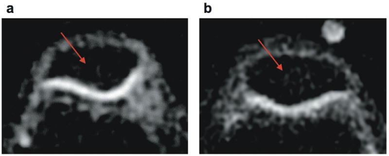
(a) Detail of standard-resolution (1.3×1.3×4.0 mm³, voxel volume of 6.8 μl) sodium image of patellar cartilage (cartilage SNR = 9). (b) Detail of high-resolution (1.0×1.0×2.0 mm³, voxel volume of 2 μl) sodium image of patellar cartilage (cartilage SNR = 8). The displayed FOV is 7×5 cm². The cartilage is distinguishable even without the aid of an anatomical proton image given its relatively high sodium content. The high-resolution image (b) shows a thinner cartilage profile given the smaller partial volume effects, yet the image quality in panel (a) is clearly better reflecting the higher SNR. This difference can be seen in the sections inside the patellar signaled by the red arrow, where image (b) exhibits more noise than panel (a).

References

- 1.Bashir A, Gray ML, Hartke J, Burstein D. Nondestructive Imaging of Human Cartilage Glycosaminoglycan Concentration by MRI. Magn Reson Med. 1999;41:857–865. doi: 10.1002/(sici)1522-2594(199905)41:5<857::aid-mrm1>3.0.co;2-e. [DOI] [PubMed] [Google Scholar]
- 2.Reddy R, Insko EK, Noyszewski EA, Dandora R, Kneeland JB, Leigh JS. Sodium MRI of Human Articular Cartilage In Vivo. Magn Reson Med. 1998;39:697–701. doi: 10.1002/mrm.1910390505. [DOI] [PubMed] [Google Scholar]
- 3.Wheaton AJ, Borthakur A, Shapiro EM, et al. Proteoglycan Loss in Human Knee Cartilage: Quantitation with Sodium MR Imaging-Feasibility Study. Radiology. 2004;231:900–905. doi: 10.1148/radiol.2313030521. [DOI] [PubMed] [Google Scholar]
- 4.Shapiro EM, Borthakur A, Gougoutas A, Reddy R. 23 Na MRI Accurately Measures Fixed Charge Density in Articular Cartilage. Magn Reson Med. 2002;47:284–291. doi: 10.1002/mrm.10054. [DOI] [PMC free article] [PubMed] [Google Scholar]
- 5.Hilal SK, Maudsley AA, Ra JB, et al. In Vivo NMR Imaging of Sodium-23 in the Human Head. J Comput Assist Tomogr. 1985;9:1–7. doi: 10.1097/00004728-198501000-00001. [DOI] [PubMed] [Google Scholar]
- 6.Clayton DB, Lenkinski RE. MR Imaging of Sodium in the Human Brain with a Fast Three-Dimensional Gradient-Recalled-Echo Sequence at 4 T. Academic Radiology. 2003;10:358–365. doi: 10.1016/s1076-6332(03)80023-5. [DOI] [PubMed] [Google Scholar]
- 7.Boada FE, Shen GX, Chang SY, Thulborn KR. Spectrally Weighted Twisted Projection Imaging: Reducing T2 Signal Attenuation Effects in Fast Three-Dimensional Sodium Imaging. Magn Reson Med. 1997;38:1022–8. doi: 10.1002/mrm.1910380624. [DOI] [PubMed] [Google Scholar]
- 8.Irarrazabal P, Nishimura DG. Fast Three Dimensional Magnetic Resonance Imaging. Magn Reson Med. 1995;33:656–662. doi: 10.1002/mrm.1910330510. [DOI] [PubMed] [Google Scholar]
- 9.Gurney PT, Hargreaves BA, Nishimura DG. Design and Analysis of a Practical 3D Cones Trajectory. Magn Reson Med. 2006;55:575–582. doi: 10.1002/mrm.20796. [DOI] [PubMed] [Google Scholar]
- 10.Liao JR, Pelc NJ. Image Reconstruction of Generalized Spiral Trajectories. Proc 4th Meeting ISMRM. 1996:359. [Google Scholar]
- 11.Liao JR, Pauly JM, Pelc NJ. MRI Using Piecewise-Linear Spiral Trajectory. Magn Reson Med. 1997;38:246–252. doi: 10.1002/mrm.1910380213. [DOI] [PubMed] [Google Scholar]
- 12.Mao W, Smith MB, Collins CM. Exploring the Limits of RF Shimming for High-Field MRI of the Human Head. Magn Reson Med. 2006;56:918–922. doi: 10.1002/mrm.21013. [DOI] [PMC free article] [PubMed] [Google Scholar]
- 13.Van de Moortele PF, Akgun C, Adriany G, et al. Destructive Interferences and Spatial Phase Patterns at 7 T with a Head Transceiver Array Coil. Magn Reson Med. 2005;54:1503–1518. doi: 10.1002/mrm.20708. [DOI] [PubMed] [Google Scholar]
- 14.Recht M, Bobic V, Burstein D, et al. Magnetic Resonance Imaging of Articular Cartilage. Clin Orthop and Rel Res. 2001;2001:S379–S396. doi: 10.1097/00003086-200110001-00035. [DOI] [PubMed] [Google Scholar]
- 15.Recht MP, Resnick D. MR Imaging of Articular Cartilage: Current Status and Future Directions. Am J Roentgenol. 1994;163:283–290. doi: 10.2214/ajr.163.2.8037016. [DOI] [PubMed] [Google Scholar]
- 16.Disler DG, Peters TL, Muscoreil SJ, et al. Fat-Suppressed Spoiled GRASS Imaging of Hyaline Cartilage: Technique Optimization and Comparison with Conventional MR Imaging. Am J Roentgenol. 1994;163:887–892. doi: 10.2214/ajr.163.4.8092029. [DOI] [PubMed] [Google Scholar]
- 17.McCauley TR, Disler DG. MR Imaging of Articular Cartilage. Radiology. 1998;209:629–640. doi: 10.1148/radiology.209.3.9844653. [DOI] [PubMed] [Google Scholar]
- 18.Beatty PJ, Nishimura DG, Pauly JM. Rapid Gridding Reconstruction with a Minimal Oversampling Ratio. IEEE Trans Med Imaging. 2005;24:799–808. doi: 10.1109/TMI.2005.848376. [DOI] [PubMed] [Google Scholar]
- 19.Gudbjartsson H, Patz S. The Rician Distribution of Noisy MRI Data. Magn Reson Med. 1995;34:910–914. doi: 10.1002/mrm.1910340618. [DOI] [PMC free article] [PubMed] [Google Scholar]
- 20.Hayes CE, Axel L. Noise Performance of Surface Coils for Magnetic Resonance Imaging at 1.5 T. Medical Physics. 1985;12:604. doi: 10.1118/1.595682. [DOI] [PubMed] [Google Scholar]
- 21.Duyn JH, Yang Y, Frank JA, van der Veen JW. Simple Correction Method for k-Space Trajectory Deviations in MRI. J Magn Reson. 1998;132:150–153. doi: 10.1006/jmre.1998.1396. [DOI] [PubMed] [Google Scholar]
Associated Data
This section collects any data citations, data availability statements, or supplementary materials included in this article.