Abstract
This paper presents a new deformable model using both population and patient-specific statistics to segment the prostate from CT images. There are two novelties in the proposed method. First, a modified scale invariant feature transform (SIFT) local descriptor, which is more distinctive than general intensity and gradient features, is used to characterize the image features. Second, an online training approach is used to build the shape statistics for accurately capturing intra-patient variation, which is more important than inter-patient variation for prostate segmentation in clinical radiotherapy. Experimental results show that the proposed method is robust and accurate, suitable for clinical application.
Keywords: Deformable model, shape statistics, segmentation, SIFT, prostate CT images
1. INTRODUCTION
Segmentation of the prostate from CT images is an important and challenging task for prostate cancer radiotherapy. The treatment is usually planned on a planning CT on which the prostate and nearby critical structures are manually contoured. The treatment is delivered in daily fractions over a period of several weeks. In modern adaptive radiation therapy (ART), a new CT image is acquired before selected individual treatments to enable adjustment of the treatment, and these images must be manually segmented. So, for one patient under treatment, we always have a manual segmented image for building the therapy plan, and the remaining problem is how to segment a series of following treatment images automatically.
The main difficulty for segmentation is the poor contrast between the prostate and the surrounding tissues, and the high variability of prostate shape. Deformable model based methods address these challenges via their ability to incorporate a priori information extracted from a training set and their flexibility to represent object shapes. They have thus been increasingly important for prostate segmentation. Two key questions need to be resolved in designing these methods:
How to select the image features and design the objective function to accurately and robustly match the deformable surface onto the object in an image.
How to build a compact statistical shape model to capture the shape variation more accurately.
The first point aims to characterize image features richly and to design the objective function to guide the model deformation. Approaches to this problem, specific to the domain of medical image segmentation, have included correlation of pixel intensities acquired along profiles normal to the object boundary [1], the quantile histograms of pixel intensities [2], and the probability distributions of photometric variables [3]. On the other hand, various features have been designed in computer vision, such as scale invariant feature transform (SIFT) [4], PCA-SIFT [5], steerable filters [6] and so on. Among these local descriptors, SIFT has been validated as one of the best performing feature sets in a recent comparative study [7] and has been successfully applied in medical object segmentation [8]. So, in our method, SIFT is used to capture image features for guiding the prostate segmentation.
For the second point, active shape models (ASM) [1] and m-reps [9] have supplied compact forms to capture the shape variability, including both inter- and intra-patient variation. In this work, we use a point-based shape model similar to ASM.
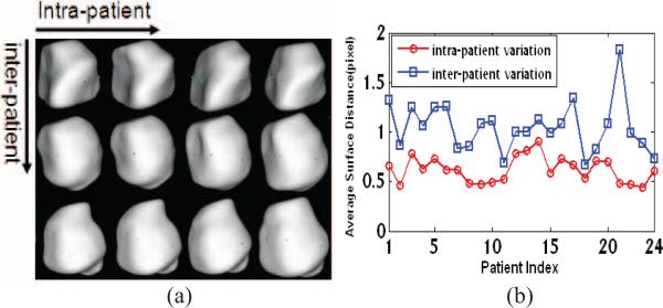
An important advantage of working with multiple images of the same patient is that the shape variation is generally much less than that between patients. This is evident in the prostate shapes of different patients shown in Fig. 1(a), where the prostates of the same patient always look more similar. We can quantify this observation using our training set of 24 anonymous patients by comparing the inter-patient average shape distance and intra-patient average shape distance (see Fig. 1(b)). So we can say that the inter-patient variation always dominates the final results of principal component analysis (PCA) in ASMs or principal geodesic analysis (PGA) in m-reps because it is larger than intra-patient variation. This makes it hard for ASMs or m-reps to capture the intra-patient variation accurately.
Fig. 1.
Comparison between intra-patient and inter-patient variation. (a) Prostate shapes of three patients at four time points. Shapes in each row are from the same patient; shapes in different columns are from different time points. (b) The average surface distances (ASD) among 24 patients. For one patient, the intra-patient ASD is the mean of distances between each shape and the mean shape of that patient, and the inter-patient ASD is the distance between the mean shape of that patient and the total mean shape of all patients.
On the other hand, for segmentation of daily treatment images, the variation within one patient is more important than the variation between patients. If, as we assume, we already have one accurate segmentation for a given patient, and if the intra-patient variation is captured accurately, the segmentation of the following images will become easier.
Others have suggested methods to eliminate the effect of inter-patient variation. Several groups have used some images coming from one patient for training, and then segmented the other images of this same patient [2,3]. Results were good, but this kind of method is limited for clinical application because there are usually not enough images of the patient under therapy to be used in the training. To overcome this problem, [10] assumes intra-patient variation is stationary across patients and pools training statistics on residues from the mean of each patient. In that approach, when a patient image is being segmented, the mean comes from the previous images of the patient being treated, and the residue model comes from the training set. When there are few images of the patient under therapy to use for training, the stationarity assumption is reasonable because there is no better choice. However, as more and more images are acquired, it makes sense to build a more accurate residue model by using the current patient's images. Based on this idea, this paper proposes an online training mechanism. At the beginning, we use the shape and appearance of the planning image as the mean shape and the mean appearance, with the residue derived from the training set as our residue model. As more images are segmented, the shape and appearance statistics are updated online, and the patient-specific information takes a larger and larger role as the number of segmented images increases.
2. METHOD
2.1. Description
Our method consists of two major parts: online training and deformable segmentation. For both of these steps, all the comparisons are made in a specified benchmark space, which we define to be the space of the planning image for the patient being treated. All images and surfaces are transformed to this benchmark space before further operation. The surfaces are transformed rigidly by a least-squares fit to the known surface already provided in the planning image. The image being segmented has a known position in the planning frame of reference, determined in the clinic.
• Online training
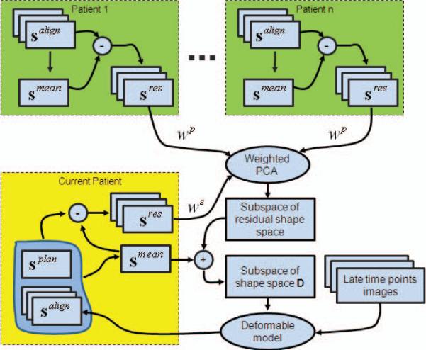
First, for a given patient, each manually generated surface of the training set is mapped to the benchmark space, yielding a surface that we denote salign. The mean shape sres of the patient is calculated, and residual shapes sres are obtained by subtracting the mean shape smean from aligned shape salign. This process is performed for the training patients and for the prior images in the patient under treatment.
Second, a weighted PCA is done to all sres with weight factor Ws for the current patient and Wp for the training set. By adjusting parameters Ws and Wp , we can control the relative weights between the patient-specific and population information flexibly.
Last, after performing weighted PCA, a reasonable residual shape space is obtained. Then, by just shifting this space using the smean of the current patient, we can get a reasonable shape space D for the current patient. Thus, D is available to guide the deformable model to segment the later time images of the current patient. In the segmentation step, we use the mean shape of the current patient as the model shape, denoted as smdl . Fig. 2 demonstrates the main procedures of online training.
Fig. 2.
Demonstration of main procedures of online training. In this figure, the blocks with green represent the population information, and the yellow one represents the patient-specific information.
It should be noted that the training is dynamic: along with each new treatment image that is segmented, smean and sres of the current patient are changed. At the same time, we decrease Wp and increase Ws gradually. Thus, as more subsequent images of the current patient are acquired, the patient-specific shape statistics collected online gain more influence.
• Deformable segmentation
The segmentation is implemented on the space of the planning image. When a new treatment image is acquired, it is rigidly transformed onto the space of the planning image of the same patient according to the pelvic bone by using the FLIRT software package. Thus, we can obtain a pose-normalized image, denoted as Inorm. It is worth noting that the model shape smdl, i.e., smean of the current patient, is in the same space with Inorm. Thus, smdl should be close to the prostate in the Inorm. For a more accurate initialization, smdl is shifted and rotated in a small scope while checking the energy function defined in Section 2.3; when this function reaches its minimum, a good initialization is obtained.
For our deformable segmentation model, we introduce SIFT features to build the appearance model (as detailed in Section 2.3). The training strategy of the appearance model is similar with that described above for the shape model. A new energy function is proposed based on these shape and appearance statistics. By optimizing this function, the initialized shape is deformed to match the pose normalized image Inorm and get a deformed shape. Then this shape is transformed to the original space of Inorm , and the final segmentation result is obtained. The energy function is detailed in Section 2.3.
2.2. SIFT Local Descriptor
SIFT features have been proven to be one of the best to represent distinctive image locations [7]. Generating SIFT features involves four major steps: (1) scale-space peak selection; (2) key point localization; (3) orientation assignment; (4) key point descriptor calculation. The first two steps detect the key points in the scale space, annd they are not required in this study since we already have the surface points along the boundaries of prostate. Therefore, we use the last two steps to compute the SIFT features for each surface point. Our approach is same as that in [8]. The dominant orientation for each point is computed based on all the gradients inside the local neighborhood around that point, and the SIFT features are computed from the histograms of gradients.
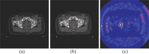
Now, we demonstrate the performance of the SIFT as a distinctive feature for prostate CT images. Fig. 3 shows that SIFT features are able to detect the corresponding points in the prostate CT images. In this figure, the SIFT features of the red crossed point in one treatment image as shown in Fig. 3(a) are compared with the SIFT features of all the points in another treatment image as shown in Fig. 3(b), by using a Euclidean distance measure between two SIFT feature vectors. As indicated by the color-coded map in Fig. 3(c), there are only a very small number of points in Fig. 3(b) similar to the red crossed point in Fig. 3(a).
Fig. 3.
Demonstration of SIFT features for correspondence detection in two different treatment images of the same patient. The SIFT features of the red crossed point in (a) is compared with the SIFT features of all the points in (b). The resultant similarity map is color-coded and shown in (c), with yellow representing high similarity. The red crossed point in (b) is the corresponding point detected, which has the highest similarity within the circular neighborhood in (c).
2.3. Deformable Segmentation Algorithm
For the deformable segmentation algorithm, we look for a surface s* by minimizing the following equation.
| (1) |
The energy term ESIFT is a distance measure between SIFT features, and minimizing it requires that the SIFT features of each surface point from the model image match the SIFT features of the corresponding point in the current treatment normalized image Inorm. For each point pi on the surface, its SIFT feature vector Vi consists of 128 elements [8]. ESIFT is defined as follows.
| (2) |
Here v̵i(l) represents the l-th element of the average SIFT feature vector of the i-th surface point in the model image space, and vi(l) is the l-th element of the SIFT feature vector of the corresponding point in the image Inorm. The quotient value σi(l) is the standard deviation estimated from the training samples. N is the total number of surface points in the deformable surface s.
Notice that the statistics of SIFT features, i.e., the average SIFT feature vectors and the standard deviation of each element, are used for feaature matching according to Eq. (2). The use of the statistics of SIFT features tends to be more robust in feature matching and less biased than the use of SIFT features from a single image. Similar to the use of the shape statistics, the average SIFT feature vector v̵i come from the current patient, while the standard deviation σi is a weighted combination of the standard deviation of the current patient and that of the training data. The weight factor is dependent on the number of images we have captured and processed from the same patient. This is consistent with the use of the patient-specific shape statistical model in our deformable segmentation procedure.
For solving Eq. (1), an iterative optimization strategy is used to compute the deformed surface by alternately miinimizing the energy term and correcting the new surface into the reasonable shape space D as described in Section 2.1. At the t-th iteration step:
First, the deformable surface st is updated via a local search around its current location, so that the newly updated surface st′ has a better match to the SIFT features of the testing image, which yields a smaller ESIFT(st′).
Second, the population-based and patient-specific shape statistics are used to constrain the newly updated deformable surface st′. A reasonable surface is obtained by finding the nearest surface to st′ in the reasonable shape space D.
Third, a new deformable surface st′ and a reasonable surface are combined by a weighted average using to get the final surface st+1 of this iteration step. The parameter ω is used to adjust the strength of the shape constraint. In this paper, ω is decreased from 0.8 to 0 according to an exponential function in the whole iterative segmentation procedure.
3. EXPERIMENT
Our data consists of 24 patient image sets, each with 12 daily CT scans of the male pelvic area taken during a course of radiotherapy. The images have an in-plane resolution of 512×512 with voxel dimensions of 0.98mm×0.98mm and an inter-slice distance of 3mm.
We are also provided expert manual segmentations of the prostate in every image. We consider the patients separately, i.e., segmenting the images from one patient in a leave-one-patient-out study. For one patient, the first treatment image is regarded as the planning image and the remaining 11 images are segmented for evaluation, so there are a total of 11×24=264 test images.
Two quantitative measures are used to evaluate the performance of the algorithms, i.e., the Dice similarity coefficient (DSC) [11] and the average surface distance (ASD) between the automated and manual segmentation results. A DSC value of 0.7 or greater is generally considered to be a high level of coincidence between segmentations [12].
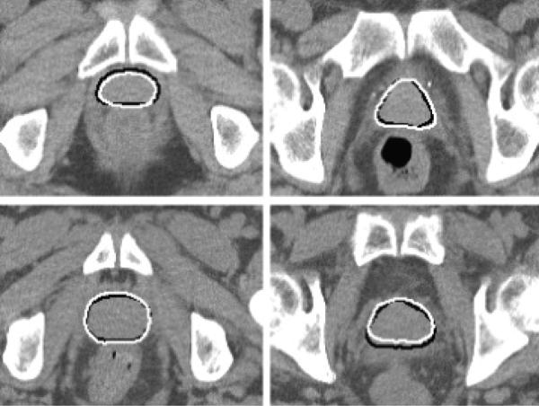
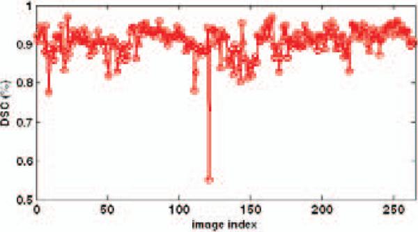
Table 1 shows the average DSC and average ASD of all 264 segmentation results using our method. It can be seen that the mean of average DSC for the prostate is 90.5%, and the mean of average ASD is 1.90 mm. Fig. 4 shows some results with the DSC around 90%. One can see that when the DSC attains 90%, the contours of the prostate given by our method are very close to those drawn by an expert. Fig. 5 shows the DSC of each image. It can be seen that only one image out of 264 has a DSC value less than 0.7, indicating the robustness of our method.
Table 1.
Average DSC and average ASD between the manual and automated segmentations of all 264 images.
| Mean ± std | Min | Median | Max | |
|---|---|---|---|---|
| Average DSC (%) | 90.5 ±4.0 | 55.1 | 91.2 | 96.9 |
| Average ASD (mm) | 1.90±0.71 | 0.84 | 1.76 | 8.35 |
Fig. 4.
Segmentation results for two slices of the 3rd treatment image of the first patient (top) and the third patient (bottom). The DSCs of these two results are 90.4% and 90.8%, respectively. The white contours show the results of our method, and the black contours show the results of manual segmentation.
Fig. 5.
DSCs of all 264 images.
Our results are comparable to those of [2,3], if slightly less accurate. More importantly, our method is the only one which is suitable for the clinical application among these three methods. For our method, only a segmented planning image is required, not a set of training images of the current patient as the methods presented in [2,3]. This point is very important for clinical application.
4. CONCLUSIONS
We have presented a new deformable model for segmenting the prostate in serial CT images by using both population-based and patient-specific statistics. The patient-specific statistics are learned online and incrementally from the segmentation results of previous treatment images of the same patient. In particular, for initial treatment images, the population-based shape statistics plays the primary role for statistically constraining the deformable surface. As more and more segmentation results are obtained, the patient-specific statistics start to constrain the segmentation and gradually take the major role for the statistical constraining. In order to facilitate the correspondence detection during the deformable segmentation procedure, the SIFT local descriptor is used to characterize the image features around each surface point. Compared to other generic features, SIFT features are relatively distinctive and thus make the correspondence detection across different treatment CT images more reliable. Experimental results show that the proposed method is robust and accurate, suitable for the clinical application.
5. ACKNOWLEDGEMENTS
This research was supported by the grants from National Natural Science Funds of China (No. 30800254 and No. 30730036).
5. REFERENCES
- 1.Cootes TF, Edwards GJ, Taylor CJ. Active Appearance Models. IEEE Transactions on Pattern Analysis and Machine Intelligence. 2001;23:681–685. [Google Scholar]
- 2.Stough JV, Broadhurst RE, Pizer SM, Chaney EL. Regional appearance in deformable model segmentation. presented at Information Processing in Medical Imaging (IPMI); 2007. [DOI] [PubMed] [Google Scholar]
- 3.Freedman D, Radke RJ, Zhang T, Jeong Y, Lovelock M, Chen GTY. Model-Based Segmentation of Medical Imagery by Matching Distributions. IEEE Transactions on Medical Imaging. 2005;24:281–292. doi: 10.1109/tmi.2004.841228. [DOI] [PubMed] [Google Scholar]
- 4.Lowe DG. Distinctive Image Features from Scale-Invariant Keypoints. International Journal of Computer Vision. 2004;60:91–110. [Google Scholar]
- 5.Ke Y, Sukthankar R. PCA-SIFT: a More Distinctive Representation for Local Image Descriptors. presented at IEEE Computer Society Conference on Computer Vision and Pattern Recognition (CVPR).2004. [Google Scholar]
- 6.Freeman WT, Adelson EH. The Design and Use of Steerable Filter. IEEE Transactions on Pattern Analysis and Machine Intelligence. 1991;13:891–906. [Google Scholar]
- 7.Mikolajczyk K, Schmid C. A Performance Evaluation of Local Descriptors. IEEE Transactions on Pattern Analysis and Machine Intelligence. 2005;27:1615–1630. doi: 10.1109/TPAMI.2005.188. [DOI] [PubMed] [Google Scholar]
- 8.Shi Y, Qi F, Xue Z, Chen L, Ito K, Matsuo H, Shen D. Segmenting Lung Fields in Serial Chest Radiographs using both Population-based and Patient-specific Shape Statistics. IEEE Transactions on Medical Imaging. 2008;27:481–494. doi: 10.1109/TMI.2007.908130. [DOI] [PubMed] [Google Scholar]
- 9.Fletcher PT, Lu C, Pizer SM, Joshi S. Principal Geodesic Analysis for the Study of Nonlinear Statistics of Shape. IEEE Transactions on Medical Imaging. 2004;23:995–1004. doi: 10.1109/TMI.2004.831793. [DOI] [PubMed] [Google Scholar]
- 10.Pizer SM, Broadhurst RE, Jeong J-Y, Han Q, Saboo R, Stough JV, Tracton G, Chaney EL. Intra-Patient Anatomic Statistical Models for Adaptive Radiotherapy. presented at MICCAI Workshop From Statistical Atlases to Personalized Models: Understanding Complex Diseases in Populations and Individuals.2006. [Google Scholar]
- 11.Dice LR. Measures of the amount of ecologic association between species. Ecology. 1945;26:297–302. [Google Scholar]
- 12.Zou KH, Warfield SK, Baharatha A, Tempany C, Kaus MR, Haker SJ, Wells WM, Jolesz FA, Kikinis R. Statistical validation of image segmentation quality based on a spatial overlap index1 scientific reports. Academic Radiology. 2004;11:178–189. doi: 10.1016/S1076-6332(03)00671-8. [DOI] [PMC free article] [PubMed] [Google Scholar]


