AUTOMATED RELIABLE LABELING OF THE CORTICAL SURFACE

Abstract

Accurate and reliable labeling of regions of interest (ROIs) within structural magnetic resonance images (MRIs) is an important step in group analysis. Group registration does not always yield accurate alignment of homologous regions. We present an approach that distinguishes itself from other algorithms by being concerned with a label which is of the highest fidelity, while leaving ambiguous regions unlabeled. Regions that are not deemed to be reliably labeled are not included in group statistics. We will present results showing that our method is an improvement over traditional multi-atlas voting schemes. We conclude with a pilot study of longitudinal trends of cortical thickness in normal aging.

1. INTRODUCTION

Recently, there have been several studies observing structural changes within specific regions of interest (ROIs) in MR brain images that are associated with both normal aging and neurological disorders [1–5]. These regional studies are either longitudinal (with respect to the individual) or cross-sectional (exploring the population as a whole) and are carried out with either a trained anatomist who manually labels structures [3, 5] or an automated labeling approach [2, 6]. Anatomists can disagree on their labels, they tend to take a very long time to label the images, and they are highly variable as individuals and across anatomists. A popular automated approach is the use of average map techniques (AMTs) [4, 7]. AMTs align cortical surface models from multiple subjects and display results on a single representation of the cortical surface with anatomical labels. The optimal approach for regional cortical analysis remains unclear; it is our belief that more accurate, consistent and detailed automatic labeling approaches are needed to propel scientific studies.

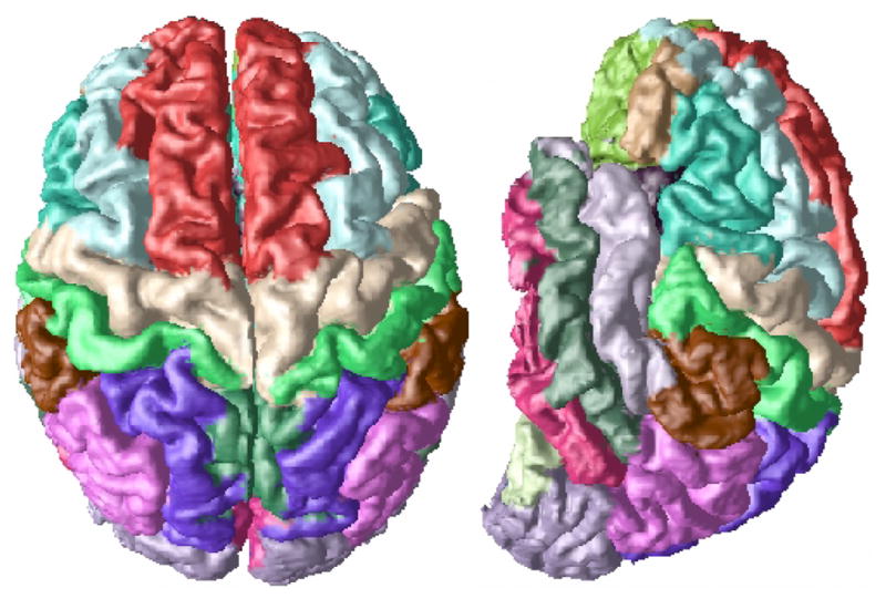
Our method is a multiple-atlas based cortical surface segmentation using a non-rigid registration algorithm based on the Adaptive Bases Algorithm (ABA) [9]. The atlases we use are manual gyral labels, Fig. 1 shows the labels on a cortical surface representation of the gray matter (GM) and cere-brospinal fluid (CSF) interface. Atlas based segmentation has been widely used for many applications [10–12]. It has been noted that with such methods there is always an increasing marginal improvement in the segmentation of the subject with each additional atlas that is used [13]. Non-rigid registration is a computationally intensive task, so any marginal improvement in the segmentation of the subject is offset by the amount of time required to garner the improvement. We will therefore combine multiple atlas registrations in a novel way to achieve improved results while avoiding unnecessary registration steps and wasted computation. In brief, our method will use what we term a reliability map, pre-computed on the atlases, to determine the labels on the subject. We do this by registering atlases with the subject and then combining the reliability maps and the labels of the atlases within the subject space to determine the labels. Our methodology is volume based, however we show results with a cortical surface representation because of the gyral basis of the labels.

Fig. 1.

Gyri-based labeling, shown on its cortical surface extracted by CRUISE [8].

In the following section, we will describe our algorithm in detail. Then we will provide results describing the accuracy of our method in comparison to a traditional multi-atlas voting scheme.

2. METHOD

Instead of generating coarse regions of interest (ROIs) [2], the purpose of our labeling is to give as many correct labels as possible. With voxels of the CSF/GM interface where there is some degree of ambiguity, we will err on the side of caution and leave the voxel unlabeled.

2.1. Reliability Map

The atlases we use to build our reliability map are T1-weighted magnetization prepared rapid gradient echo (MP-RAGE) data with two sagittal acquisitions being averaged to increase the contrast-to-noise ratio. Originally the data contained 33 labels per hemisphere, some of these labels were determined to be inconsistently identified. Such labels were merged with an appropriate adjacently labeled region, to form a superset of 20 labels per hemisphere, Table 1 shows a list of the labels. We used 17 such atlases to build our reliability map; a more detailed description of the acquisition and how the subjects were originally labeled is available in [14].

Table 1.

LH AC and RH AC denote the left and right hemisphere annual change, which is in mms per year.

Gyral Label	LH AC	RH AC
Superiortemporal	−0.0340***	−0.0344***
Superiorfrontal	−0.0315***	−0.03200***
Middletemporal	−0.0284***	−0.0153**
Supramarginal	−0.0280***	−0.0188***
Inferiorfrontal	−0.0269***	−0.0222***
Inferiorparietal	−0.0256***	−0.0250***
Parsorbitalis	−0.0239***	−0.0243***
Middlefrontal	−0.0227***	−0.0281***
Superiorparietal	−0.0222***	−0.0192***
Inferiortemporal	−0.0199***	−0.0177**
Postcentral	−0.0192***	−0.0130***
Precentral	−0.0161***	−0.0169***
Cingulate Region	−0.0161***	−0.0152***
Lingual	−0.0154***	−0.0108**
Precuneus	−0.0149***	−0.0124**
Lateraloccipital	−0.0132***	−0.0140***
Orbitofrontal	−0.0119**	−0.0112**
Fusiform	−0.0119*	−0.0072
Cuneus	−0.0072***	−0.0056*
Parahippocamal	−0.0034	−0.0094

^*corresponds to a p value less than 0.05,

^**a p value less than 0.01 and

^***a p value less than 0.001.

A reliability map associated with an atlas brain, , has values [0, 1] on each voxel v of , describing how reliably this voxel can be mapped to a subject brain. We create a reliability map for each atlas brain in the following manner:

Given N atlases, , , …, with corresponding labels ℒ_i(v) for the voxel v within . We obtain by registering against each of , …, , using the Adaptive Bases Algorithm (ABA). ABA registration maximizes mutual information with an underlying deformation field modeled on radially symmetric basis functions. We denote by , registered to , i = 2, …, N. ℒ_1i(v) is derived by deforming ℒ₁(v) by the corresponding deformation field. We then define , as an evaluation of the alignment of ℒ_1i(v) against ℒ_i(v), by

$${\mathcal{R}}_{{\mathcal{A}}_1}(v)=\frac{\sum _{i=2}^N\delta ({\mathcal{L}}_{1i}(v),{\mathcal{L}}_i(v))}{N-1},$$

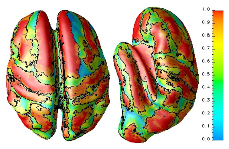
where, δ(a, b) is the Kronecker delta. A reliability value of 1 at a voxel means that the voxel has been mapped into the correct region for the N − 1 atlases. For each atlas we can compute this reliability map, relative to the other N − 1 atlases, before we try to label a subject data set. Fig. 2 shows an example of a reliability map that has been mapped to the GM/CSF interface from the 3D reliability map.

Fig. 2.

Reliability map shown on a partial inflated GM/CSF interface. The partial inflation enables viewing of deep sulcal regions. The black contours correspond to a reliability value of 0.8.

2.2. Labeling

For each atlas we have labels, ℒ_i(v), and the reliability map, , for all voxels v of . We then proceed to label a given subject, , using M atlases, with M < N, as follows:

1. Register the M atlases to and compute a voting score on each voxel that receives a given label. Let denote the result of transforming the labels ℒ_i(v) into using the corresponding deformation field and denotes the transformed reliability map. is the voting score that v receives the label j and is defined as,

   $$\mathcal{V}(v\mid j)=\sum _{i=1}^M\delta ({\mathcal{L}}_{i\mathcal{S}}(v),j){\mathcal{R}}_{i\mathcal{S}}(v),$$

   where j = 1, …, K, with K being the total number of labels in the atlas. For each voxel choose a candidate label, l, defined as, l = argmax {j : }.

2. For the candidate label, compute the average reliability value,

   $$\mathcal{R}(v)=\frac{{\displaystyle \sum _{i=1}^M}\delta ({\mathcal{L}}_{i\mathcal{S}}(v),l){\mathcal{R}}_{i\mathcal{S}}(v)}{{\displaystyle \sum _{i=1}^M}\delta ({\mathcal{L}}_{i\mathcal{S}}(v),l)}.$$

Assign the voxel v with the label l if ℛ(v) is larger than a threshold t, otherwise we leave the voxel unlabeled. More formally,

$${\mathcal{L}}_{\mathcal{S}}(v)=\{\begin{array}{ll}l,\hfill & \text{if}\mathcal{R}(v)\ge t,\hfill \\ 0,\hfill & \text{otherwise}.\hfill \end{array}$$

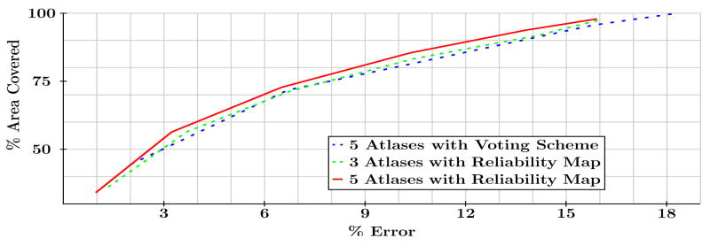
We will discuss how to choose t in the next section. We choose M so as to reduce the number of registrations required without affecting the accuracy of the results, see Fig. 3 for example.

Fig. 3.

% Area covered plotted against the % label error for our method with 3 and 5 atlases and for VS with 5 atlases. Our approach with 3 atlases is indistinguishable from the VS method with 5 atlases.

3. RESULTS

As an initial experiment we compare our algorithm against some ground truth atlases. From the population of 17 data sets that built our reliability map we draw an additional 17 subjects, different from the atlas data but acquired and labeled in an identical fashion.

For comparison we implemented a voting scheme (VS) [15] approach which registered M′ MP-RAGE atlas subjects to the 17 subjects to be labeled and assigned labels based on a majority voting scheme with thresholding. Fig. 3 shows the performance curves of the two labeling schemes were we have varied the threshold of the voting scheme and the threshold t in our approach to create these curves. Lowering the thresholds gives larger labeled surface area while diminishing the quality of those labels. Our approach when compared to VS with the same number of atlases (5) improved the covered area by 5% at the same error level. Our method with M = 3 is almost identical to VS with more atlases, M′ = 5.

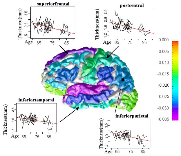
We demonstrate the usefulness of these reliably labeled regions by considering the effects of aging on the thickness of the cerebral cortex. We use the same data as [1], in which the authors semi-automatically labeled 4 sulcal regions, per hemisphere, on 35 subjects (16 men and 19 women) from the Baltimore Longitudinal Study of Aging (BLSA) [16], with subjects ages ranging from 50 to 84 years. Five acquisitions for each subject, with an approximate one year interval between scans, were labeled using our approach. Our reliability map is the same as used in the previous experiment, with a threshold t = 0.80. Thickness measurements were taken in each of our ROIs based on [17]. We then access the relationship between the ROIs median thickness and age, in order to match the statistical analysis used in [1], we used a simple linear regression model. Annual changing rates of thickness in millimeters per year are shown in Fig. 4.

Fig. 4.

Thickness trends for four ROIs. The color bar on the right is the scale for the change in thickness based on a simple linear regression model. Areas in white are unlabeled and are not accessed as part of the regression.

The previous work on this data could only identify two regions which showed statistically significant changes in thickness, in contrast we have 37 regions which show significant changes. The regions and the change in thickness are shown in Table 1, significance of the p-value is also denoted. The thinning rate for the postcentral and precentral gyrus corresponds with the results from the earlier study for the ROI referred to as the central sulcus. The thinning trends also agree with the common belief that there is more gray matter loss in the association cortex than the primary sensory cortex. In particular the prefrontal, entorhinal and temporal cortices are the most severely affected by aging [18, 19].

4. DISCUSSION AND CONCLUSION

We have presented a fully automated gyral labeling scheme which is an improvement over the traditional voting scheme approach. Our algorithm also has computational benefits over other multi-atlas approaches. By incorporating the reliability map we can reduce the number of registrations required while not impacting the quality of the results. This method shows potential for improving longitudinal based studies of aging, not just for thickness as in our experiments but for all cortical related measures that require ROIs.

References

- 1.Rettmann ME, et al. Cross-sectional and longitudinal analyses of anatomical sulcal changes associated with aging. Cerebral Cortex. 2006;16(11):1584–1594. doi: 10.1093/cercor/bhj095. [DOI] [PubMed] [Google Scholar]
- 2.Sowell ER, et al. Sex differences in cortical thickness mapped in 176 healthy individuals between 7 and 87 years of age. Cerebral Cortex. 2007;17(7):1550–1560. doi: 10.1093/cercor/bhl066. [DOI] [PMC free article] [PubMed] [Google Scholar]
- 3.Raz N, et al. Regional brain changes in aging healthy adults: General trends, individual differences and modifiers. Cerebral Cortex. 2005;15(11):1676–1689. doi: 10.1093/cercor/bhi044. [DOI] [PubMed] [Google Scholar]
- 4.Salat DH, Buckner RL, Snyder AZ, Greve DN, Desikan RS, Busa E, Morris JC, Dale AM, Fischl B. Thinning of the cerebral cortex in aging. Cerebral Cortex. 2004;14(7):721–730. doi: 10.1093/cercor/bhh032. [DOI] [PubMed] [Google Scholar]
- 5.Luders E, Narr KL, Thompson PM, Rex DE, Jancke L, Toga AW. Hemispheric asymmetries in cortical thickness. Cerebral Cortex. 2006;16(8):1232–1238. doi: 10.1093/cercor/bhj064. [DOI] [PubMed] [Google Scholar]
- 6.Resnick SM, Pham DL, Kraut MA, Zonderman AB, Davatzikos C. Longitudinal magnetic resonance imaging studies of older adults: A shrinking brain. J of Neuroscience. 2003;23(8):3295–3301. doi: 10.1523/JNEUROSCI.23-08-03295.2003. [DOI] [PMC free article] [PubMed] [Google Scholar]
- 7.Gogtay N, et al. Dynamic mapping of human cortical development during childhood through early adulthood. Proc Nat Acad Sci. 2004;101(21):8174–8179. doi: 10.1073/pnas.0402680101. [DOI] [PMC free article] [PubMed] [Google Scholar]
- 8.Han X, Pham DL, Tosun D, Rettmann ME, Xu C, Prince JL. CRUISE: Cortical reconstruction using implicit surface evolution. NeuroImage. 2004;23:997–1012. doi: 10.1016/j.neuroimage.2004.06.043. [DOI] [PubMed] [Google Scholar]
- 9.Rohde GK, Aldroubi A, Dawant BM. The adaptive bases algorithm for intensity based nonrigid image registration. IEEE Trans Med Imag. 2003;22:1470–1479. doi: 10.1109/TMI.2003.819299. [DOI] [PubMed] [Google Scholar]
- 10.Fischl B, et al. Whole brain segmentation: Automated labeling of neuroanatomical structures in the human brain. Neuron. 2002;33(3):341–355. doi: 10.1016/s0896-6273(02)00569-x. [DOI] [PubMed] [Google Scholar]
- 11.Thompson PM, Toga AW. Detection, visualization and animation of abnormal anatomic structure with a deformable probabilistic brain atlas based on random vector field transformations. Medical Image Analysis. 1997;1(4):271–294. doi: 10.1016/s1361-8415(97)85002-5. [DOI] [PubMed] [Google Scholar]
- 12.Collins DL, Zijdenbos AP, Baaré WFC, Evans AC. ANIMAL + INSECT: Improved cortical structure segmentation; Information Processing in Medical Imaging: 16th International Conference, IPMI’99; Springer; 1999. pp. 210–223. [Google Scholar]
- 13.Rohlfing T, Brandt R, Menzel R, Maurer CR., Jr Evaluation of atlas selection strategies for atlas-based image segmentation with application to confocal microscopy images of bee brains. NeuroImage. 2004;21(4):1428–1442. doi: 10.1016/j.neuroimage.2003.11.010. [DOI] [PubMed] [Google Scholar]
- 14.Desikan RS, et al. An automated labeling system for subdividing the human cerebral cortex on mri scans into gyral based regions of interest. NeuroImage. 2006;31(3):968–980. doi: 10.1016/j.neuroimage.2006.01.021. [DOI] [PubMed] [Google Scholar]
- 15.Parhami B. Voting algorithms. IEEE Trans Reliability. 1994;43(4):617–629. [Google Scholar]
- 16.Shock NW, Greulich RC, Andres R, Arenberg D, Costa PT, Jr, Lakatta E, Tobin JD. Normal human aging: The Baltimore Longitudinal Study of Aging. U.S. Government Printing Office; Washington, D.C: 1984. [Google Scholar]
- 17.Han X, Xu C, Tosun D, Prince JL. Proc Work Math Meth Biomed Image Anal. Springer; 2001. Cortical surface reconstruction using a topology preserving geometric deformable model; pp. 213–220. [Google Scholar]
- 18.Kemper TL. Neuroanatomical and neuropathological changes during aging and dementia. In: Albert ML, editor. Clinical neurology of aging. Oxford University Press; 1984. pp. 3–67. [Google Scholar]
- 19.Raz N. Neuroanatomy of aging brain: evidence from structural MRI. In: Bigler ED, editor. Neuroimaging II Clinical applications. Springer; 1996. pp. 153–182. [Google Scholar]