Improved Radial GRAPPA Calibration for Real-Time Free-Breathing Cardiac Imaging

Abstract

In order to generate real-time, non-gated, free-breathing cardiac images, the undersampled radial trajectory combined with parallel imaging in the form of radial GRAPPA has shown promise. However, this method starts to fail at high undersampling factors due to the assumptions that must be made for the purposes of calibrating the GRAPPA weight sets. In this manuscript, a novel through-time radial GRAPPA calibration scheme is proposed which greatly improves image quality for the high acceleration factors required for real-time cardiac imaging. This through-time calibration method offers better image quality than standard radial GRAPPA, but it requires many additional calibration frames to be acquired. By combining the through-time calibration method proposed here with the standard through-k-space radial GRAPPA calibration method, images with high acceleration factors can be reconstructed using few calibration frames. Both the through-time and the hybrid through-time/through-k-space methods are investigated to determine the most advantageous calibration parameters for an R=6 in vivo short-axis cardiac image. Once the calibration parameters have been established, they are then used to reconstruct several in vivo real-time, free-breathing cardiac datasets with temporal resolutions better than 45ms, including one with a temporal resolution of 35ms and an in-plane resolution of 1.56mm².

INTRODUCTION

The use of cardiac magnetic resonance imaging (MRI) to non-invasively assess heart function has increased in recent years due to advances in imaging speed and image reconstruction methods [1-6]. The most commonly employed technique is gated and segmented cine imaging, which assumes a regular heart beat and limited patient motion. However, this method fails when the cardiac motion is not steady (arrhythmias or physiological variation), or when the patient cannot comply with breath-hold commands. In such cases, the examination must either be repeated, or the physician must use the limited data that can be acquired. Thus, real-time cardiac imaging, which does not require ECG gating or breath-holds, has become a subject of great interest.

The challenge in real-time cardiac imaging is in balancing the fundamental trade-off between temporal and spatial resolution. In order to adequately capture cardiac motion, the total image acquisition time should be on the order of 50 ms or less, a timing which corresponds to a frame rate of 20 frames per second. Using the conventional steady-state free precession (SSFP) sequence with a TR of approximately 2.5 ms and standard Cartesian sampling, the number of phase encoding lines which can be acquired is limited to fewer than 20. The spatial resolution is therefore also constrained by the temporal limitation unless post-processing schemes are employed.

Parallel imaging in the form of SENSE [7-8] and GRAPPA [9] can be used to facilitate real-time cardiac imaging by reducing the number of phase encoding lines required for a given spatial resolution [7]. For instance, in one of the earliest works to use SENSE for cardiac imaging, a maximum reduction factor of 3.2 was employed, yielding image matrices of 128×116 after SENSE reconstruction with a temporal resolution of 27ms/frame. Other works have demonstrated that acceleration factors of up to 6 or 7 are possible using a 32-channel receiver coil [10,11], but further acceleration in 2D imaging is generally not possible because of the SNR loss due to the geometry factor. Higher acceleration factors have been demonstrated in 3D by accelerating in both the phase and partition encoding directions [12]. For the standard versions of these parallel imaging methods, a low resolution calibration dataset must also be acquired in order to determine either the coil sensitivity map needed for SENSE or the reconstruction weights needed for GRAPPA. This can be avoided by using special formulations of SENSE/GRAPPA for dynamic imaging, namely TSENSE or TGRAPPA [13,14]. While these post-processing methods allow the acquisition of images with a spatial and temporal resolution that show cardiac anatomy and motion, the artifacts in the form of noise enhancement and residual aliasing can be prominent and detract from the overall image quality, especially for reduction factors above R=4. Methods that take advantage of the spatiotemporal correlations inherent in the semi-regular cardiac movement, such as UNFOLD or k-t BLAST, have been shown to offer even higher data reduction factors [14,16], but are plagued by temporal blurring. Thus, even when applying several different methods simultaneously (i.e., k-t SENSE or k-t GRAPPA [15-17]), robust acceleration factors of greater than R=8 are difficult to achieve in 2D cardiac imaging using standard rectilinear sampling.

Another way to acquire images rapidly is to employ non-Cartesian trajectories, such as the radial or spiral trajectory. Several authors have shown that these trajectories allow for a more efficient coverage of k-space and fewer motion artifacts, especially for cardiac imaging [18-23]. In addition, these trajectories can be undersampled with fewer malicious aliasing artifacts than Cartesian sampling. Using the radial trajectory with undersampling, acceleration factors of between 2 and 3 can be employed without any other post-processing for cardiac imaging without introducing artifacts which are detrimental to the image quality [21-23]. However, even when employing radial undersampling, it is difficult to achieve a temporal resolution of less than 50 ms while obtaining sufficient data for a clinically relevant spatial resolution and low artifact power.

The cardiac imaging option explored here is a combination of the above mentioned methods; namely, parallel imaging and non-Cartesian imaging. To this end, a novel form of radial GRAPPA is described and applied to accelerated real-time, free-breathing in vivo cardiac images. This method, introduced in its original form by Griswold, et al in 2003 [24], was first shown to be applicable for dynamic, and especially cardiac, imaging in 2004 [25]. Radial GRAPPA is advantageous due to the high acceleration factors that can be achieved without obtrusive aliasing artifacts, thereby allowing a higher temporal and spatial resolution for cardiac imaging. However, in practice, the original formulation of radial GRAPPA with high acceleration factors has proven challenging due to the calibration scheme proposed in these early works. In order to collect enough data for calibration, a fully-sampled data set must be acquired and segmented along the projection and read directions; weight sets can then be calculated using these segments and applied to the portion of the undersampled data with the same geometry. Assuming that the coil array exhibits sufficient sensitivity variation to perform the reconstruction, the segmentation necessary for the calibration can lead to either blurring (when the segments are too large) or noise enhancement (when the segments are too small). Thus, other options for the calibration of radial GRAPPA have been sought.

To answer this challenge, several techniques have been examined. For instance, by using the fully-sampled central portion of k-space acquired as part of the undersampled radial acquisition, one can synthesize estimates of the missing projections [26-29]. The undersampled data can also be used directly to calculate radial GRAPPA weights after an interpolation step [30]. While these methods no longer require a fully-sampled radial dataset, they all require segmentation of the synthesized fully-sampled estimate, which leads to the same problems described for the original formulation of radial GRAPPA. Other parallel imaging methods, namely conjugate gradient SENSE [31], PARS [32], pseudo-Cartesian GRAPPA [33], and APPEAR [34], have also been proposed for the reconstruction of undersampled non-Cartesian data. However, the undersampling factors demonstrated for these methods generally do not exceed R=4, which is not fast enough for the frame rates required for real-time cardiac imaging.

In this paper, we revisit the original radial GRAPPA method and introduce a calibration scheme which does not require segmentation or interpolation, yielding exact GRAPPA weights for each kernel geometry. This method is examined and applied to real-time free-breathing cardiac data. This exact calibration method and one that uses additional segmentation are compared to standard radial GRAPPA using highly undersampled short axis cardiac data in order to determine the optimal reconstruction parameters for this application. The conclusions drawn from these reconstructions are then applied to generate accelerated real-time, free-breathing cardiac images with temporal resolutions better than 45ms.

THEORY

Cartesian GRAPPA

The principle of radial GRAPPA is similar to standard Cartesian GRAPPA, which works as described here. In order to reduce experiment time, some phase encoding lines are skipped. Then, to reconstruct the missing data, the effects of gradient encoding are mimicked using the spatial variations in the multi-channel receiver coil used to collect the data. This is accomplished by forming a weighted linear combination of acquired points (the source points) in order to generate the missing k-space points (the target points).

In Cartesian GRAPPA, a reconstruction kernel size and geometry must be selected. This kernel describes the distribution of the source points relative to the target points, and is usually made up of points in both the phase and read direction (and partition in the case of 3D GRAPPA); 2×3 or 4×5 kernels (phase × read) are commonly used in 2D imaging. The source points are multiplied by a weight set and summed, resulting in the value of the target point for each receiver coil. Because GRAPPA is a coil-by-coil reconstruction, this process is repeated for each of the target points for each coil. Assuming a 2×3 kernel and acceleration in the ky-direction by a reduction factor of R, this process can be written as:

$${\tilde{s}}_{\mathrm{targ},i}(k_x,k_y+\Delta k_y)=\sum _{j=1}^{\mathit{NC}}\sum _{{\tau }_x}\sum _{{\tau }_y}n(i,j,{\tau }_x,{\tau }_y)\cdot s_{\mathrm{src},j}(k_x+{\tau }_x,k_y+{\tau }_y)$$

where s̃_targ,i(k_x, k_y + Δk_y) is the estimate of the target point to be reconstructed in the i^th receiver coil, s_src,j(k_x + τ_x, k_y + τ_y) represents a source point in the kernel from coil j, τ_x and τ_y indicate the positions in the kernel (for a 2×3 kernel, τ_x is [−1 0 1] and τ_y is [0 R]), and n(i,j,τ_x,τ_y) is the value of the GRAPPA weight set for the proper target and source coils and position in the kernel. Given NC independent receiver channels in the array and N_b points in the kernel (N_b=6 for the 2 × 3 kernel), the weights set is usually organized to have a size of [NC,NC·N_b]. This equation can be simplified by writing it in matrix notation:

$${\tilde{S}}_{\mathrm{targ}}=\widehat{w}\cdot S_{\mathrm{src}}$$

where S_src refers to the vector containing the kernel source points for each coil, S̃_targ is the vector containing the estimated target points for each coil, and ŵ is the GRAPPA weight set for the arrangement of source and target points selected. This GRAPPA weight set can be determined by acquiring several additional k-space lines (known as the auto-calibration signal, or ACS) such that both the target points and the source points are known:

$$s_{\mathrm{targ},i}(k_x,k_y+\Delta k_y)=\sum _{j=1}^{\mathit{NC}}\sum _{{\tau }_x}\sum _{{\tau }_y}n(i,j,{\tau }_x,{\tau }_y)\cdot s_{\mathrm{src},j}(k_x+{\tau }_x,k_y+{\tau }_y)$$

In this equation, s̃_targ,i(k_x, k_y + Δk_y) has been replaced by s_targ,i(k_x, k_y + Δk_y) to denote that the target points are known and not estimates, as in the reconstruction. The weight set can then be calculated by collecting all of the occurrences of the source and target points in the appropriate kernel arrangement through the ACS, placing them in large source and target point matrices, and performing a pseudo-inverse (pinv). The actual calculation is easiest shown using the matrix formulation:

$$\widehat{w}={\widehat{S}}_{\mathrm{ACS},\mathrm{targ}}\cdot \mathrm{pinv}\left({\widehat{S}}_{\mathrm{ACS},\mathrm{src}}\right)$$

It is important to note that in order to be able to accurately calibrate the weight set, many occurrences of the kernel through the ACS are needed to assure that the calibration equation is fully determined. At least NC·N_b occurrences of the kernel are required to make the equation exactly determined, and using more further increases the stability of the weight set.

Original Radial GRAPPA—through k-space calibration

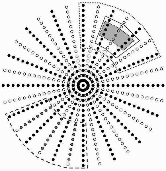
Unlike in Cartesian GRAPPA and as shown in Figure 1, a single kernel cannot be defined in an undersampled radial dataset due to the changing degree and direction of undersampling in the radial trajectory. However, there are areas in k-space where the kernels are similar, if not exactly the same. The initial formulation of radial GRAPPA makes the assumption that the weight sets for these kernels will also be similar to one another, and that the weight set for all of the data in a given segment can be calibrated using a segment from a fully-sampled dataset. Once the weights for each segment have been determined and applied to the undersampled radial data, the reconstructed radial data can be gridded to arrive at the reconstructed image.

Figure 1.

R=2 radial dataset (a single coil shown), where the black points have been acquired and the white points must be reconstructed. Although a separate fully-sampled dataset is used for the calibration, the segments that are appropriate for such a calibration are shown on the undersampled data. The 2 × 3 GRAPPA kernel is demarked with a dotted line and gray shading. For calibration, a large segment with 35 patterns (9 × 7 in the read × projection directions, surrounded by the dotted line) can be used. However, the assumption that the patterns is no longer valid. Using a smaller segment (the 6 × 3 segment, solid line) leads to patterns that are similar, but the calibration system of equations may be less overdermined (or even underdetermined). This figure also shows the difference between the original standard radial GRAPPA, and that used here. In the original version, all target points falling within a segment are reconstructed using the weights derived from that segment (bottom left, dashed segment). In this work, only a single point, in the center of the segment, was reconstructed for each segment (top right, dotted segment).

In order to perform the calibration, a fully-sampled radial dataset is used in standard radial GRAPPA. The projections acquired in the undersampled dataset must be a subset of those acquired in the calibration dataset, and the spacing between the projections must be equidistant to allow the segmentation approximation. The degree of segmentation for the reconstruction can be changed according to the size of the data matrix and the reduction factor. These through-k-space segments can be different sizes along the read and projection direction. For instance, because there is less variation in the size and shape of the kernel along the read direction than in the projection direction, it may be advantageous to use a kernel that is larger in this direction. In general, using smaller segments assures that the kernels within the segment have a similar geometry, as the approximation of parallel lines within a segment breaks down as the segment increases in size.

However, the number of kernel occurrences through the segment to be used as the ACS must be at least as large as the number of points in the kernel times the number of receiver coils. Thus, for increasing acceleration factors, where the segments should be kept small so that the kernel geometry is similar, care must be taken to ensure that the number of kernel occurrences in the segment is large enough to allow an accurate determination of the weights. For instance, using a base matrix size of 128×128, an undersampled radial acquisition with 32 projections (or R=4 with respect to the Cartesian case), and a reference radial scan with 128 projections, dividing the undersampled radial data into 64 total segments (of size 16 projection × 16 read) and using a 2 × 3 kernel results in only 168 occurrences of the kernel in each segment. One can calculate how many occurrences there are by examining how many times the 2×3 kernel fits into the segment; there are 12 occurrences along the projection direction for R=4 and 14 in the read direction (not 16 and 16 because of the size of the kernel in both directions), leading to a total of 168 occurrences of the kernel. Therefore, with a 15 channel receiver coil and a kernel size of 6 points, the calibration equation would be only slightly overdetermined, leading to weights which are highly influenced by noise in the data and which may not accurately represent the coil sensitivities. It is also important to note that these segments are rather large, each encompassing 45° in the radial k-space, and the approximation of a constant kernel orientation and size no longer holds. Moving to a larger segment to increase the number of occurrences of the kernel in the segment necessarily leads to further inaccuracies.

These issues have lead to several constraints when performing standard radial GRAPPA. Firstly, small kernels (2×3) are generally used to maximize the number of kernel occurrences through the segment for the calibration. Secondly, large segments are chosen for the same reason, although the central approximation of radial GRAPPA is made invalid by the use of such large segments. This second problem is especially detrimental with large reduction factors, which often cannot be calibrated and reconstructed properly. These constraints have limited the use of radial GRAPPA when performing the calibration with this through-k-space scheme.

In the original formulation of radial GRAPPA, once the segments are defined and the weights for each segment determined, all of the missing points within that segment are calculated using the same weight set. However, it is also possible to perform a separate calibration for each missing point by centering a segment of a given size around that specific point. This means that many more weight sets must be determined, but the segments more accurately reflect the acceleration distance and degree and the reconstruction is improved as compared to the case where all of the points within a segment are reconstructed with a single weight set.

Through-Time Radial GRAPPA Calibration

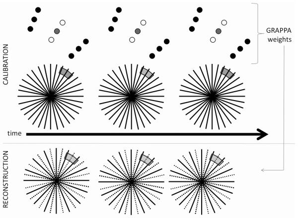
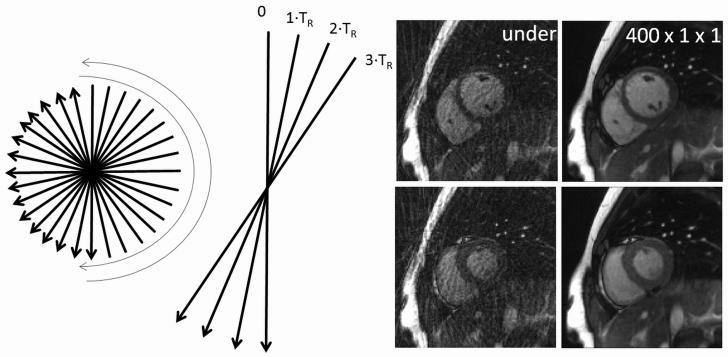
Due to the difficulties inherent in using the k-space segmentation calibration scheme described above, a new method was examined for the calibration of the radial GRAPPA weights. In addition to the accelerated scan, a set of fully-sampled radial scans are acquired and employed for the GRAPPA calibration. Then, instead of using multiple regions in k-space to collect enough information for calibration, multiple repetitions in time can be used, as depicted in Figure 2. In this way, no segmentation is required, and each missing point can be calibrated using a through-time kernel that fits precisely to the spatial harmonics of the acquired points. Because most of the residual artifacts in radial GRAPPA occur due to the segmentation scheme, it is expected that this through-time calibration method leads to better image quality at higher acceleration factors. Although this method potentially requires the acquisition of several fully-sampled datasets, these data can be acquired even when significant motion (i.e. cardiac, breathing) is present. This is due to the fact that the projections used for the calibration of each kernel are acquired in a sequential fashion, such that little motion occurs during the time required for their acquisition (~(R+1)·T_R) (see Figure 3). Thus, as long as the motion between sequential k-space projections is minimal, it is irrelevant that the images in the calibration phase contain motion (and motion artifacts).

Figure 2.

A schematic of the through-time radial GRAPPA method. Top: Several fully sampled radial datasets are acquired sequentially; here, single patterns which occur only once in k-space appear several times throughout the multiple repetitions. These repetitions (specific pattern of source and target points shown above) are used to calibrate the specific GRAPPA weight set for that pattern. Bottom: Once the weights for the specific pattern have been calculated, they can be applied in the appropriate k-space location in undersampled data. The same process is repeated for each missing point in the undersampled radial trajectory.

Figure 3.

Left: the metronome radial trajectory used in this work to avoid off-resonance artifacts in the True-FISP sequence due to large jumps in k-space. Radial projections are acquired sequentially first in one direction, and then in the opposite direction. Center: although significant cardiac and respiratory motion can occur during the acquisition of an entire k-space, little motion occurs between the acquisition of adjacent projections, as very little time passes between one line and the next. Right: Example undersampled images (left) for the 24-projection in vivo dataset in diastole and systole, and the corresponding reference images (right) reconstructed using the through-time radial GRAPPA method with 400 calibration frames and no k-space segmentation.

The major drawback of a purely through-time calibration is that many fully-sampled radial datasets are required. For instance, if through-time calibration were used instead of the segmentation in the example in the previous section, a total of 168 fully-sampled datasets would be required. This may not be acceptable in clinical applications.

Hybrid Through-Time/Through-k-Space Radial GRAPPA Calibration

As stated above, the main problem with a purely through-time radial GRAPPA calibration is the number of fully-sampled radial frames which must be acquired to determine the weight sets. One simple way to reduce the number of fully-sampled frames needed is to employ a hybrid through-time/through-k-space method, where small segments are employed to boost the number of times the kernel appears for the calibration. Here, the extension of the pure through-time calibration method using different sizes of segments is examined and it is demonstrated that the introduction of small segments may preserve a high quality reconstruction with fewer calibration frames than a pure through-time calibration.

METHODS

In vivo cardiac data were acquired with healthy volunteers in compliance with our institution's IRB on a Siemens 1.5T Espree scanner (Siemens Medical Solutions, Erlangen, Germany) and a standard 12-channel cardiac receiver coil. A radial bSSFP sequence was employed. In order to prevent eddy current artifacts, a metronome-like radial projection ordering was developed, which allowed projections adjacent in time to also be adjacent in k-space (this trajectory is shown schematically in Figure 3). This sequence was used for the collection of calibration as well as undersampled data. The fully-sampled data were made up of 400 frames, with the following parameters (also listed in Table 1): FoV = 200mm², base matrix size = 128², spatial resolution = 1.56×1.56 mm², independent receiver channels = 12, projections/frame = 144, readout points = 256, TE/TR = 1.46ms/2.92ms, bandwidth = 1000 Hz/pixel, flip angle = 45°. A total of 100 undersampled frames were collected using similar parameters, but the number of projections was decreased to 24 per frame, corresponding to an acceleration factor of R=5.3 with respect to the Cartesian case. This leads to a frame rate of 14.3 frames/s. It is important to note that the projections in the accelerated data must be a subset of the fully-sampled data, which is why a total of 144 projections were acquired for the calibration data although a 128² matrix was reconstructed (24 divides evenly into 144, but not 128). All data, both calibration and undersampled, were acquired without cardiac gating during free-breathing. Examples of undersampled images (in diastole and systole) are shown on the right-hand side of Figure 3 to demonstrate the severity of the artifacts.

Table 1.

Parameters for the various in vivo experiments described in this manuscript.

	Figures 3-5	Figure 6	Figure 7	Figure 8	Figure 9	Figure 10
Base Matrix	128	128	128	128	128	128
Calibration Proj	144	132	128	128	140	144
Undersampled Proj	24	22	16	16	14	12
Acceleration Factor (wrt Cartesian)	5.3	5.8	8	8	9.1	10.7
Acceleration Factor (wrt Nyquist)	8.4	9.1	12.6	12.6	14.4	16.8
TR (ms)	2.92	NA	2.86	2.7	2.86	2.92
TE (ms)	1.5	NA	1.43	1.35	1.43	1.46
FoV (mm2)	200	NA	300	350	300	200
BW (Hz/pixel)	1000	NA	1000	1000	1000	1000
Spatial Resolution (mm2)	1.56	NA	2.34	2.73	2.34	1.56
Temporal Resolution (ms)	70.08	NA	45.76	43.2	40.04	35.04
Number of Calibration Frames	varied	200	75	25	25	75
Calibration Scan Time (s)	varied	NA	27.46	8.64	10.01	31.54

The standard radial GRAPPA method was implemented as described in [24], with a slight modification. Unlike the original formulation of radial GRAPPA, the segments were centered on each missing point; while this greatly increases the calibration and reconstruction time because a separate weight set is calculated for each missing point, the reconstruction quality is improved. Despite this difference from the original method, the technique of using pure k-space segmentation and a single frame for the calibration will be known throughout this work as “standard radial GRAPPA.” For the through-time calibration method and the hybrid through-time/through-k-space method, the calibration dataset included several fully-sampled images, denoted with each reconstruction. As in the standard radial GRAPPA, the segment was centered on the missing point, such that the target point was always at the center of the segment used for calibration. It should be noted that the number of source points per coil was set at six in order to minimize the number of variables to be examined in this analysis; this means the weight set for each target point and receiver coil contained a total of 72 values (12 coils × 6 source points per coil). A standard 2 × 3 (projection × read) kernel was selected. Because no “truth” image is available, the image reconstructed through-time radial GRAPPA with the largest number of through-time kernel occurrences (400 repetitions) was used as the reference. These reference images in diastole and systole are shown in Figure 3.

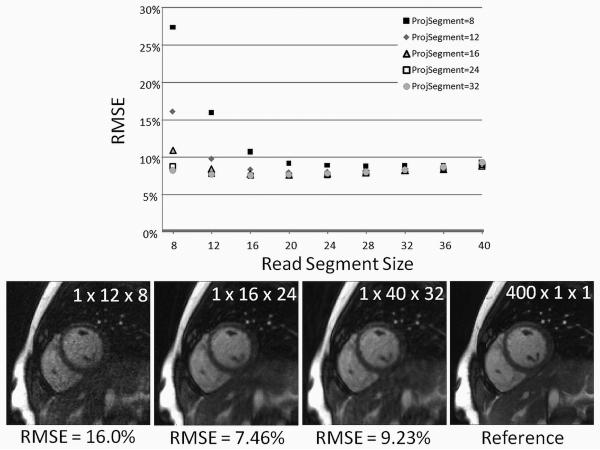
Several different reconstructions were performed for this in vivo dataset to determine the effects of different calibration schemes. First, a series of experiments was conducted to determine the effects of changing the segment size when using a single frame for calibration. In order to investigate this effect, reconstructions for the undersampled dataset were performed using one calibration frame and varying the segment size in both the read and projection directions. The k-space segments were set to sizes of [8,12,16,24,32] in the projection direction, and [8,12,16,20,24,28,32,36, 40] in the read direction. The reconstructed images were then compared with the reference simulated images, and the RMSE calculated and plotted as a function of the segment sizes.

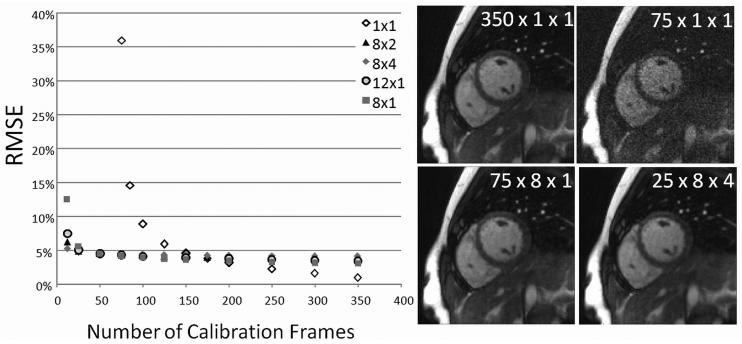
Secondly, the effect of using only a through-time calibration (with no through-k-space segmentation) with different numbers of calibration frames was examined. This analysis shows how changing the number of occurrences of the kernel effects the reconstruction. The number of calibration frames was set to [75,85,100,125,150,175,200,250,300,350]. The minimum number of frames was set to 75, as there are 72 values in the weight set for each target point; fewer calibration frames would lead to underdetermined weight sets. Each of these reconstructions using purely through-time radial GRAPPA was assessed using the reference image.

In order to reduce the number of calibration frames needed, a small amount of k-space sharing can be reintroduced to the through-time calibration, leading to the hybrid through-time/through-k-space method. Experiments were performed using the simulated data to determine whether this k-space segmentation can lead to better results (for a given number of calibration frames) than through-time GRAPPA. To this end, segment sizes of [1,2,4,8,12] were employed in both the read and projection directions along with different numbers of calibration frames. The effects of the different segment sizes were examined, and the RMSE values were compared to the through-time and standard radial GRAPPA methods to determine whether this hybrid scheme leads to improved radial GRAPPA reconstructions.

Due to the through-time nature of the calibration, it could be possible that some object information is retained in the weight sets and transferred from the calibration dataset to the undersampled dataset. To investigate whether this contrast transfer occurs, a two modified Shepp-Logan phantoms with random contrast and motion of the various ovals were generated. These phantom images were modified using a simulated eight-element one-ring head coil array, where the sensitivities were derived using an analytic integration of the Biot-Savart equations. Examples of these calibration datasets can be seen in Figure 6. Undersampled data of similar contrast to one of the calibration datasets were generated using 22 projections for the 128² image and the same coil sensitivities. It is important to note that the undersampled images appeared in neither calibration dataset. In a first step, one calibration dataset was used to reconstruct the undersampled image with a similar contrast; then the other calibration dataset (with a different contrast) was used for the reconstruction. For both reconstructions, 200 time frames were employed, and no through-k-space segmentation was used. The results of these reconstructions were then compared visually to determine whether the contrast from the calibration data affected the outcome of the reconstructions.

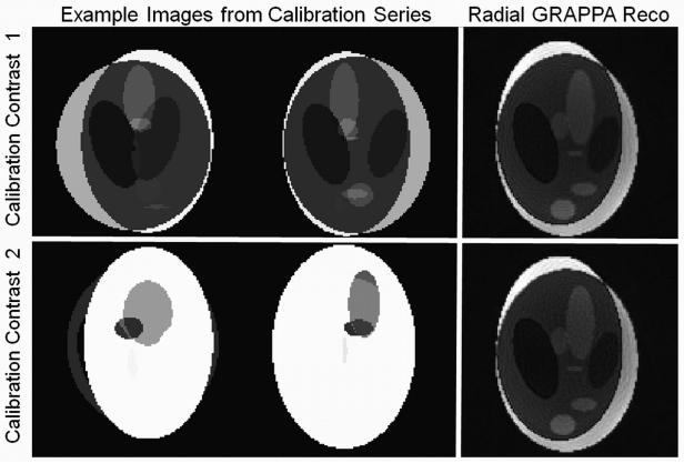
Figure 6.

Top left: Example calibration images with one contrast. Bottom left: Example calibration images with a different contrast. Top right: Image reconstructed from 22 projections with the first set of calibration data where the contrast is similar. Top bottom: Image reconstructed from 22 projections with the second set of calibration data where the contrast is different. Note that the images reconstructed with the two different contrast calibration datasets appear similar.

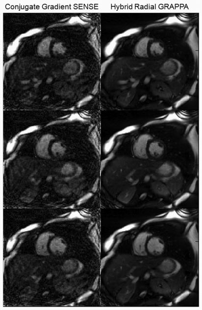
In order to demonstrate the advantage of using hybrid radial GRAPPA over CG SENSE, images were reconstructed using both methods. To this end, both a 128-projection dataset and a 16-projection dataset were acquired as the calibration and undersampled data (acquisition details given in Table 1). In the hybrid radial GRAPPA reconstruction, 75 calibration frames were employed with a segment size of 4×1 in the read and projection directions. For the CG SENSE reconstruction, coil sensitivity maps were calculated using the adaptive combine method [35] on the image generated by averaging the 75 calibration frames. The hybrid radial GRAPPA method was implemented as described here, and the CG SENSE method as described in [8].

After the results of these extensive reconstructions were examined, several additional datasets with increased frame rate and acceleration factor were acquired. The acquisition and reconstruction parameters for this datasets are given in Table 1. The goal of this study was to show that the new radial GRAPPA calibration methods can be used to reconstruct images with high temporal resolutions (35 ms to 43.2 ms) accurately during free breathing conditions with clinically acceptable calibration scan times. Reconstructions were performed using hybrid GRAPPA with parameters as suggested from the results of the analysis described above.

RESULTS

Figure 4 shows a plot of the RMSE of the images reconstructed with standard radial GRAPPA in comparison to the reference image for different segment sizes. Additionally, several example images are shown to demonstrate the image quality. As can be seen, the RMSE decreases initially with increasing segment size, indicating that larger segments lead to better reconstructions. However, as the segment further increases in size, the reconstructions begin to have a higher RMSE and worse image quality. For this dataset, the optimal reconstruction in terms of RMSE was generated using a projection segment containing 16 occurrences of the kernel and a read segment including 24 points (RMSE = 7.46%).

Figure 4.

Top: A plot of the RMSE of various reconstructions vs. read segment size for several different projection segment sizes when using standard radial GRAPPA. The best reconstruction (with the lowest RMSE, 7.46%) is the 16 × 24 (read × projection) segment size. Bottom: Example reconstructions using different segment sizes and standard radial GRAPPA. When using only a single time frame and a segment size of 12 × 8 (left), the reconstruction appears noisy and has a high RMSE. Increasing the segment size decreases this noise, but leads to blurry images with residual artifacts. The best standard radial GRAPPA image is shown in the center left, and for comparison the reference image is included on the right.

Figure 5 shows a plot of the RMSE for the 24-projection in vivo through-time radial GRAPPA reconstructions when using different numbers of calibration frames. As the number of calibration frames increases, the RMSE decreases monotonically, as expected. As this weight calculation matrix becomes less overdetermined, the reconstruction error increases, and the images contain more noise. In particular, the RMSE when employing 125 frames (5.90%) is still lower than the reconstructions with the lowest RMSE for the standard radial GRAPPA (7.46%).

Figure 5.

A plot of the RMSE vs. the number of calibration frames for through-time radial GRAPPA (segments of 1×1, shown in white diamonds) and hybrid radial GRAPPA. As the number of calibration frames decreases, the RMSE for through-time radial GRAPPA increases. By using small k-space segments in hybrid radial GRAPPA, this RMSE increase can be tempered. Right top: Example images reconstructed using through-time radial GRAPPA; as the number of calibration frames decreases, the image quality also decreases. Right bottom: Example images reconstructed using hybrid radial GRAPPA. Images with improved quality using fewer calibration frames can be reconstructed using this method as compared to the through-time method.

The RMSE values of images reconstructed using the hybrid through-time/through-k-space approach and different segment sizes are plotted in Figure 5. Employing the hybrid method leads to improved reconstructions as compared to the through-time method when fewer than 150 time frames are available for calibration. However, if more than 150 fully-sampled frames can be acquired, the through-time calibration leads to lower RMSE values than the hybrid method. The only significant differences between the different segment sizes in the hybrid through-time/through-k-space method occurs when very few frames are used for calibration.

Figure 6 demonstrates that images reconstructed using a calibration dataset with a different contrast do not take on the contrast of the calibration dataset. Both the image reconstructed using similar contrast calibration data and that reconstructed using different contrast calibration data exhibit slight SNR losses and residual blurring, but they do not appear to have different contrast behaviors. Thus, the through-time radial GRAPPA calibration method can be used to reconstruct undersampled images that differ significantly from the data used for the calibration.

Figure 7 shows several images in different cardiac phases resulting from the hybrid radial GRAPPA reconstruction as well as the CG SENSE reconstruction. While the hybrid radial GRAPPA images no longer contain aliasing artifacts, the CG SENSE images show both residual aliasing as well as additional artifacts introduced due to the mismatch between the coil sensitivity map and the undersampled image.

Figure 7.

Left: Representative images reconstructed using CG SENSE. Right: Representative images reconstructed using hybrid radial GRAPPA.

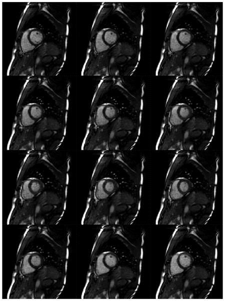
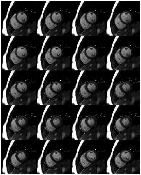
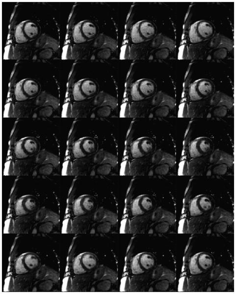
The results of the additional in vivo cardiac studies are shown in Figures 8 through 10. In Figure 8, an in vivo dataset with 16 projections (R=8 with respect to Cartesian) was reconstructed using 25 calibration frames and the hybrid calibration method with segments sizes of 8×4. The resulting temporal resolution was 43.2ms/frame (23.1 frames/s), and the spatial resolution was 2.73mm². The calibration scan lasted 8.64 sec, followed by the acquisition of 100 accelerated time frames in 4.32 seconds, so the entire free-breathing, non-gated scan lasted slightly less than 13 seconds. Figure 9 shows images reconstructed from a 14-projection dataset (R=9.1 with respect to Cartesian) also using the hybrid method with 25 calibration frames and segments of size 8×4. Again, the calibration lasted approximately 10 seconds, and the entire scan (calibration and acquisition of accelerated data) was less than 15 seconds. The frame rate of this scan was 25 frames/s, and the spatial resolution 2.34 mm². Finally, Figure 10 shows an example of a 12-projection dataset (R=10.7 with respect to Cartesian) with a temporal resolution of 35 ms (28.5 frames/s). The FoV was chosen to be 200mm², yielding a spatial resolution of 1.56mm². Due to the high spatial resolution and acceleration factor, slight residual artifacts can be seen in the reconstructions, which were performed using hybrid radial GRAPPA with 75 calibration frames and 8×1 sized segments. The calibration phase lasted 31.5 sec, and the total scan was slightly more than 35 sec. During all acquisitions, the volunteers were instructed to breathe freely, and no ECG gating was employed.

Figure 8.

Example images reconstructed from data containing 16 projections/frame with a spatial resolution of 2.73mm² and a temporal resolution of 43.2ms/frame. Hybrid radial GRAPPA was used with 25 calibration frames (requiring a calibration scan time of 8.64s), and 8×4 sized k-space segments.

Figure 10.

Example images reconstructed from data containing 12 projections/frame with a spatial resolution of 1.56mm² and a temporal resolution of 36ms/frame. Hybrid radial GRAPPA was used with 75 calibration frames (requiring a calibration scan time of 32.4s), and 8×1 sized k-space segments.

Figure 9.

Example images reconstructed from data containing 14 projections/frame with a spatial resolution of 2.34mm² and a temporal resolution of 40ms/frame. Hybrid radial GRAPPA was used with 25 calibration frames (requiring a calibration scan time of 9.94s), and 8×4 sized k-space segments.

DISCUSSION

The reconstructions performed here show that using a through-time calibration method in conjunction with radial GRAPPA can greatly improve the quality of highly undersampled radial images. The standard radial GRAPPA uses a single fully-sampled frame and through-k-space segments for calibration. By increasing the size of the segment in k-space, both in the read and projection directions, the reconstruction quality improves (RMSE decreases). This improvement comes from the fact that using larger k-space segments leads to a more overdetermined system of equations for the weight set. However, as the segment size increases, the source points within the kernel no longer have the same geometry. This leads to weights that do not properly reflect the spatial harmonic relationships between the source points and the target points, and the reconstruction quality decreases. For the in vivo dataset reconstructed here, the optimal segment size (which is large enough for an overdetermined calibration matrix yet not so large that the assumptions of radial GRAPPA break down), was 16 × 24 (read × projection). This reconstruction yields a RMSE of 7.46%. Although this is the best reconstruction (as determined by RMSE) that can be obtained using standard radial GRAPPA, the images appear blurry due to the relatively large k-space segment size. Decreasing the size of the segment leads to sharper images (albeit considerably noisier), and increasing the segment size further decreases the spatial resolution (yielding blurrier images).

Instead of relying on kernels which are similar, but not exactly the same in k-space, as in standard radial GRAPPA, through-time radial GRAPPA uses a single pattern in k-space through multiple frames. This way of calibrating makes no assumptions about the symmetry of k-space, leading to improved reconstruction quality. One drawback of the through-time radial GRAPPA method is that many fully-sampled frames are required for the calibration in order to generate an overdetermined system of equations for the GRAPPA weights. Figure 5 shows that as the number of calibration frames decreases, the quality of the reconstructed image decreases. The SNR of the images decreases (see Figure 5), as the calibration equations are less overdetermined, and noise in the individual source points begins to influence the values in the weight sets. Thus, when using purely through-time radial GRAPPA, it is advantageous to acquire many fully-sampled frames. The reference images used here employed 400 frames, which led to calibration equation systems which were 5.5 times oversampled. However, when employing fewer frames (125, or 1.7 times oversampled), the RMSE of the images reconstructed with through-time radial GRAPPA is still lower than those reconstructed using standard radial GRAPPA.

The main drawback to through-time radial GRAPPA is the large number of fully-sampled calibration frames required for the reconstruction. Since this data can be acquired in a completely free breathing acquisition, we believe that this will only really be a limitation in cases where one wishes to rapidly change slice orientation, such as in interventional imaging, or when moving to 3D radial-type acquisitions. One alternative to using a completely through-time calibration is to form small k-space segments, as in standard GRAPPA, in a hybrid through-time/through-k-space radial GRAPPA. Because some through-time calibration is still employed, the segments do not have to be as large as those in standard GRAPPA, allowing the assumption of similar kernel configurations inside the segment to be better fulfilled. Figure 5 shows that by increasing the k-space segment from 1×1 (read × projection) to 8×1 and using only 75 calibration frames, the RMSE of the reconstruction can be decreased from 5.9% to 3.5%. Thus, when using numbers of calibration frames which are on the order of the size of the GRAPPA weight set, it is advantageous to use a small amount of segmentation in the read direction. However, in the 24-projection in vivo dataset examined here, segmentation in the projection direction increased the RMSE when using greater than 75 frames (note, for instance, the higher RMSE values for 8×4 or 8×2 segments than for the 8×1 segment). This indicates that the assumption of similar kernel configurations is more realistic when using a segment which is longer in the read direction than in the angular direction. However, read segments can also become too large, which can be seen in the higher RMSE values for the 12×1 segment compared with the 8×1 segment. Additionally, when a large number of calibration frames (>200) is employed, the use of the hybrid method did not improve the image quality above the through-time calibration method. This indicates that the hybrid method should only be used in cases where the system of calibration equations is close to being exactly determined, and the use of segmentation (which is always only an approximation) cannot be avoided to generate an overdetermined system.

On the other hand, when using fewer frames than values in the weight set such that the through-time method would be underdetermined, it appears to be useful to employ segments that extend in both the read and projection directions. The results in Figure 6 indicate that segmenting along the read direction alone does not allow enough equations to be collected for an accurate determination of the weights. Thus, when using very small numbers of calibration frames, segmentation in both directions must be applied; to further emphasize this point, one can imagine that in the limit of only one calibration frame, hybrid radial GRAPPA breaks down to standard radial GRAPPA, and segmentation in both directions is necessary to collect enough equations for calibration. As in standard radial GRAPPA, when the segments must be larger, the resulting images tend to be blurrier than when using small segments. However, because hybrid GRAPPA allows smaller segment sizes, the quality of the reconstructed images is higher than in standard radial GRAPPA, as reflected in a lower RMSE (5.25% vs. 7.46%). Hence, the use of some through-time calibration is clearly better than relying on a single calibration frame.

Another alternative to the calibration phase would be to use a TGRAPPA-like approach [14], where the undersampled data are acquired in an interleaved fashion such that they can be combined to form fully-sampled datasets. In this implementation, no additional calibration frames would be required, removing the need for extra calibration scans. While this T-radial GRAPPA method may improve the amount of time needed for calibration, initial results indicate that this method may suffer due to the changes that occur from frame to frame, leading to inconsistent calibration data. However, this option has not been fully explored and will be examined in future work.

The quantitative results here have been derived using an in vivo cardiac dataset containing 24 projections/frame acquired with 12 independent receiver channels. While general statements can be made about the size of segments that should be used for an optimal radial GRAPPA calibration, the optimal segment size and most efficient number of calibration frames depends on many factors, including the acceleration factor used, the underlying SNR of the data, the number and arrangement of receiver coils, etc. The SNR is especially significant when examining the number of calibration frames and kernel occurrences necessary for reconstruction, as a low SNR in the periphery of k-space can lead to inaccurate weights in any radial GRAPPA calibration method. In lower SNR datasets, more kernel occurrences would be required in order to extract the coil sensitivity information from the edges of k-space; this must be noted when adapting this work to other applications. For the real-time, free breathing cardiac application shown here, the best reconstructions (as judged visually) were generated using 400 calibration frames and no segmentation. This led to a calibration time of 168.2 seconds (400 repetitions × 144 projections × 2.92ms), which is too long for many applications. Reconstructions similar in visual quality with a modest RMSE increase were generated using 75 calibration frames (and an 8×1 k-space segmentation), yielding a calibration scan time of 31.5s. While this is an improvement over the almost 3 minute calibration time for pure through-time radial GRAPPA, it is still quite long. By moving to segmentation in the projection direction as well as the read direction, the number of calibration frames could be reduced to 25, yielding a calibration scan time of 10.5s. While the reconstruction using hybrid radial GRAPPA with segmentation in both the read and projection directions led to images that had a slightly higher RMSE than those generated using 75 calibration frames, they are visually still of high quality, and significantly better than images generated using only one calibration frame. Thus, in order to avoid having to perform a separate analysis for each undersampled image, enough calibration frames should be acquired to provide a completely determined system of calibration equations (i.e. at least 72 for the example shown here), and then the through-time calibration should be augmented using segmentation in the read direction. If this is impossible due to time constraints, segmentation should be performed in both the read and projection directions with the maximum number of calibration frames that can be acquired. It is important to note that for the cardiac application shown here, no breathholding was required, which meant that long calibration times can be employed without undue stress on the subject.

Following these calibration suggestions, several highly accelerated cardiac datasets were acquired and reconstructed using the hybrid radial GRAPPA method. These highly accelerated datasets (with temporal resolutions between 35 ms and 43.2 ms) depict real time cardiac motion, and do not rely on a regular heartbeat or breathholding. For the lower acceleration factors and spatial resolutions, the entire scan time, including the acquisition of the calibration frames, was 15 s for a single slice. For the highest spatial and temporal resolution image, the calibration scan lasted slightly over 30 s. These images could not have been generated with standard radial GRAPPA due to the high acceleration factor and the subsequent blurring and streaking in the reconstructions.

As shown in Figure 7, the hybrid radial GRAPPA yields images with less residual aliasing than CG SENSE. This is primarily due to the fact that the CG SENSE method requires a coil sensitivity map, which is difficult to accurately acquire under the free-breathing, non-gated conditions used here. Such sensitivity maps will rarely exhibit the same cardiac phase and breathing state as the undersampled data, leading to additional artifacts from the data mismatch. For this reason, the hybrid radial GRAPPA will generally offer better image quality than methods which require a coil sensitivity map, like CG SENSE.

It should be noted that the contrast of the calibration images and the undersampled images do not have to be identical. This is demonstrated in Figure 6, and has also been shown in the context of relaxometry in [36]. This is due to the fact that both through-time and through-k-space GRAPPA both attempt to access the coil sensitivity information in order to perform the GRAPPA reconstruction. Ideally, the GRAPPA weight set would contain only information about the coil sensitivity, which is the same in all portions of k-space. This information can be gathered using multiple identical kernels through k-space (as in Cartesian GRAPPA) or in identical kernels through-time. In both cases, the underlying coil sensitivities are constant. In the second case, while the underlying images are different, the coil sensitivities are still constant. It is important to note that the calibration approaches are different; through-k-space calibration involves data from different spatial harmonics, making the method potentially more stable than through-time calibration, where it is possible that the occurrences of the kernel differ only in their noise content. However, both methods should allow one to access the coil sensitivity information and perform a reconstruction that depends on parallel imaging without making use of any knowledge of the temporal dynamics of the motion. For this reason, the contrast of the calibration data should not affect the contrast of the reconstructed image. Thus, the hybrid radial GRAPPA method can be applied to acquisitions where it is difficult to obtain the desired contrast for the calibration data, such as contrast-enhanced examinations. Here, only the undersampled data must be acquired during contrast administration; the calibration data can be acquired either before or after the injection of contrast.

Although the through-time and hybrid methods have been proposed here for radial trajectories, these methods can easily be extended to other trajectories, such as spiral. Similarly, a three-dimensional version of this method can be employed for undersampled stack-of-stars trajectories. The only requirement for such a method is that the adjacent k-space points are acquired within a short temporal window.

CONCLUSION

The through-time radial GRAPPA method presented here, along with its extension, hybrid through-time/through-k-space radial GRAPPA, has been shown to yield improved images over standard radial GRAPPA. The specific application demonstrated here, real-time cardiac imaging without breathholding or cardiac gating, was performed at temporal resolutions of 36ms and spatial resolutions of 1.56mm². It was demonstrated that, if possible, enough calibration time frames should be acquired to make the calibration equation at least solvable (i.e. at least [NC × source points] frames should be used), although it is possible to use larger k-space segmentation in hybrid radial GRAPPA if this suggestion cannot be employed due to time constraints. In addition to the real-time cardiac imaging shown here, through-time radial GRAPPA can be used for other trajectories and applications, making it potentially useful in a variety of applications where a high frame rate is required.

REFERENCES

- 1.Wieben O, Francois C, Reeder SB. Cardiac MRI of ischemic heart disease at 3 T: Potential and challenges. European Journal of Radiology. 2008;65:15–28. doi: 10.1016/j.ejrad.2007.10.022. [DOI] [PubMed] [Google Scholar]
- 2.Scharf M, Brem MH, Wilhelm M, Schoepf UJ, Uder M, Lell MM. Cardiac magnetic resonance assessment of left and right ventricular morphologic and functional adaptations in professional soccer players. Am Heart J. 2010 May;159(5):911–8. doi: 10.1016/j.ahj.2010.02.027. [DOI] [PubMed] [Google Scholar]
- 3.Sandner TA, Theisen D, Bauner KU, Picciolo M, Reiser MF, Wintersperger BJ. Kardiale Funktionsanalyse mittels MRT. Der Radiologe. doi: 10.1007/s00117-010-1987-8. Epub 7 May 2010. [DOI] [PubMed] [Google Scholar]
- 4.Babar JL, Jones RG, Hudsmith L, Steeds R, Guest P. Application of MR Imaging in Assessment and Follow-up of Congenital Heart Disease in Adults. Radiographics. doi: 10.1148/rg.e40. Epub 12 May 12 2010. [DOI] [PubMed] [Google Scholar]
- 5.Liu J, Spincemaille P, Codella NC, Nguyen TD, Prince MR, Wang Y. Respiratory and cardiac self-gated free-breathing cardiac CINE imaging with multiecho 3D hybrid radial SSFP acquisition. Magn Reson Med. 2010 May;63(5):1230–7. doi: 10.1002/mrm.22306. [DOI] [PMC free article] [PubMed] [Google Scholar]
- 6.Duarte S, Bogaert J. The role of cardiac magnetic resonance in hypertrophic cardiomyopathy. Rev Port Cardiol. 2010 Jan;29(1):79–93. [PubMed] [Google Scholar]
- 7.Pruessmann KP, Weiger M, Scheidegger MB, Boesiger P. SENSE: sensitivity encoding for fast MRI. Magn Reson Med. 1999 Nov;42(5):952–62. [PubMed] [Google Scholar]
- 8.Pruessmann KP, Weiger M, Boesiger P. Sensitivity encoded cardiac MRI. J Cardiovasc Magn Reson. 2001;3(1):1–9. doi: 10.1081/jcmr-100000143. [DOI] [PubMed] [Google Scholar]
- 9.Griswold MA, Jakob PM, Heidemann RM, Nittka M, Jellus V, Wang J, Kiefer B, Haase A. Generalized autocalibrating partially parallel acquisitions (GRAPPA) Magn Reson Med. 2002 Jun;47(6):1202–10. doi: 10.1002/mrm.10171. [DOI] [PubMed] [Google Scholar]
- 10.Wintersperger BJ, Reeder SB, Nikolaou K, Dietrich O, Huber A, Greiser A, Lanz T, Reiser MF, Schoenberg SO. Cardiac CINE MR imaging with a 32-channel cardiac coil and parallel imaging: impact of acceleration factors on image quality and volumetric accuracy. J Magn Reson Imaging. 2006;23:222–7. doi: 10.1002/jmri.20484. [DOI] [PubMed] [Google Scholar]
- 11.Fenchel M, Deshpande VS, Nael K, Finn JP, Miller S, Ruehm S, Laub G. Cardiac cine imaging at 3 Tesla: initial experience with a 32-element body-array coil. Invest Radiol. 2006;41:601–8. doi: 10.1097/01.rli.0000223896.70095.49. [DOI] [PubMed] [Google Scholar]
- 12.Hardy CJ, Cline HE, Giaquinto RO, Niendorf T, Grant AK, Sodickson DK. 32-Element receiver-coil array for cardiac imaging. Magn Reson Med. 2006;55:1142–9. doi: 10.1002/mrm.20870. [DOI] [PMC free article] [PubMed] [Google Scholar]
- 13.Kellman P, Epstein FH, McVeigh ER. Adaptive sensitivity encoding incorporating temporal filtering (TSENSE) Magn Reson Med. 2001;45:846–852. doi: 10.1002/mrm.1113. [DOI] [PubMed] [Google Scholar]
- 14.Breuer FA, Kellman P, Griswold MA, Jakob PM. Dynamic autocalibrated parallel imaging using temporal GRAPPA (TGRAPPA) Magn Reson Med. 2005 Apr;53(4):981–5. doi: 10.1002/mrm.20430. [DOI] [PubMed] [Google Scholar]
- 15.Guttman MA, Kellman P, Dick AJ, Lederman RJ, McVeigh ER. Realtime accelerated interactive MR imaging with adaptive TSENSE and UNFOLD. Magn Reson Med. 2003;15:315–321. doi: 10.1002/mrm.10504. [DOI] [PMC free article] [PubMed] [Google Scholar]
- 16.Tsao J, Kozerke S, Boesiger P, Pruessmann KP. Optimizing spatiotemporal sampling for k-t BLAST and k-t SENSE: application to high-resolution real-time cardiac steady-state free precession. Magn Reson Med. 2005 Jun;53(6):1372–82. doi: 10.1002/mrm.20483. [DOI] [PubMed] [Google Scholar]
- 17.Huang F, Akao J, Vijayakumar S, Duensing GR, Limkeman M. k-t GRAPPA: a k-space implementation for dynamic MRI with high reduction factor. Magn Reson Med. 2005 Nov;54(5):1172–84. doi: 10.1002/mrm.20641. [DOI] [PubMed] [Google Scholar]
- 18.Ahn CB, Kim JH, Cho ZH. High-speed spiral-scan echo planar NMR imaging. IEEE Trans Med Imaging. 1986;5:2–7. doi: 10.1109/TMI.1986.4307732. [DOI] [PubMed] [Google Scholar]
- 19.Meyer CH, Hu BS, Nishimura DG, Macovski A. Fast spiral coronary artery imaging. Magn Reson Med. 1992;28:202–213. doi: 10.1002/mrm.1910280204. [DOI] [PubMed] [Google Scholar]
- 20.Glover GH, Pauly JM. Projection reconstruction techniques for reduction of motion effects in MRI. Magn Reson Med. 1992;28:275–289. doi: 10.1002/mrm.1910280209. [DOI] [PubMed] [Google Scholar]
- 21.Schaeffter T, Weiss S, Eggers H, Rasche V. Projection reconstruction balanced fast field echo for interactive real-time cardiac imaging. Magn Reson Med. 2001 Dec;46(6):1238–41. doi: 10.1002/mrm.1322. [DOI] [PubMed] [Google Scholar]
- 22.Boll DT, Merkle EM, Seaman DM, Gilkeson RC, Larson AP, Simonetti OP, Duerk JL, Lewin JS. Comparison of ECG-gated rectilinear vs. real-time radial K-space sampling schemes in cine True-FISP cardiac MRI. J Cardiovasc Magn Reson. 2004;6(4):793–802. doi: 10.1081/jcmr-200036124. [DOI] [PubMed] [Google Scholar]
- 23.Peters DC, Rohatgi P, Botnar RM, Yeon SB, Kissinger KV, Manning WJ. Characterizing radial undersampling artifacts for cardiac applications. Magn Reson Med. 2006 Feb;55(2):396–403. doi: 10.1002/mrm.20782. [DOI] [PubMed] [Google Scholar]
- 24.Griswold MA, Heidemann RM, Jakob PM. Direct parallel imaging reconstruction of radially sampled data using GRAPPA with relative shifts; Proceedings of the 11th Annual Meeting of the ISMRM; Toronto, Canada. 2003. p. 2349. [Google Scholar]
- 25.Griswold MA, Blaimer M, Heidemann RM, Speier P, Kannengeiser S, Nittka M, Breuer F, Mueller M, Jakob PM. Rapid Evaluation of Cardiac Function Using Undersampled Radial TrueFISP with GRAPPA; Proceedings of the 12th Annual Meeting of the ISMRM; Kyoto, Japan. 2004. p. 737. [Google Scholar]
- 26.Breuer FA, Seiberlich N, Blaimer M, Jakob PM, Griswold MA. Quantitative g-factors for radial GRAPPA; Proceedings of the 17th Annual Meeting of the ISMRM; Honolulu, Hawaii, USA. 2009. p. 2712. [Google Scholar]
- 27.Samsonov AA, Block WF, Arunachalam A, Field AS. Advances in locally constrained kspace-based parallel MRI. Magn Reson Med. 2006;55(2):431–438. doi: 10.1002/mrm.20757. [DOI] [PubMed] [Google Scholar]
- 28.Arunachalam A, Samsonov A, Block WF. Self-calibrated GRAPPA method for 2D and 3D radial data. Magn Reson Med. 2007;57(5):931–938. doi: 10.1002/mrm.21223. [DOI] [PubMed] [Google Scholar]
- 29.Huang F, Vijayakumar S, Li Y, Hertel S, Reza S, Duensing GR. Self-calibration method for radial GRAPPA/k-t GRAPPA. Magn Reson Med. 2007;57(6):1075–1085. doi: 10.1002/mrm.21233. [DOI] [PubMed] [Google Scholar]
- 30.Codella NCF, Spincemaille P, Prince M, Wang Y. A Rapid Self-Calibrating Radial GRAPPA method using Kernel Coefficient Interpolation; Proceedings of the 3rd International Third International Workshop on Parallel MRI; Santa Cruz, CA. 2009. [Google Scholar]
- 31.Pruessmann KP, Weiger M, Boernert P, Boesiger P. Advances in sensitivity encoding with arbitrary k-space trajectories. Magn Reson Med. 2001;46:638–651. doi: 10.1002/mrm.1241. [DOI] [PubMed] [Google Scholar]
- 32.Yeh EN, McKenzie CA, Ohliger MA, Sodickson DK. Parallel magnetic resonance imaging with adaptive radius in k-space (PARS): constrained image reconstruction using k-space locality in radiofrequency coil encoded data. Magn Reson Med. 2005 Jun;53(6):1383–92. doi: 10.1002/mrm.20490. [DOI] [PubMed] [Google Scholar]
- 33.Seiberlich N, Breuer F, Heidemann R, Blaimer M, Griswold M, Jakob P. Reconstruction of undersampled non-Cartesian data sets using pseudo-Cartesian GRAPPA in conjunction with GROG. Magn Reson Med. 2008 May;59(5):1127–37. doi: 10.1002/mrm.21602. [DOI] [PubMed] [Google Scholar]
- 34.Beatty PJ, Hargreaves BA, Gurney PT, Nishimura DG. A Method for Non-Cartesian Parallel Imaging Reconstruction with Improved Calibration; Proceedings of the 15th Annual Meeting of the ISMRM; Berlin, Germany. 2007. p. 335. [Google Scholar]
- 35.Walsh DO, Gmitro AF, Marcellin MW. Adaptive reconstruction of phased array MR imagery. Magn Reson Med. 2000 May;43(5):682–90. doi: 10.1002/(sici)1522-2594(200005)43:5<682::aid-mrm10>3.0.co;2-g. [DOI] [PubMed] [Google Scholar]
- 36.Kunth M, Seiberlich N, Ehses P, Gulani V, Griswold M. Improvement of Quantitative MRI using Radial GRAPPA in Conjunction with IR-TrueFISP; Proceedings of the 18th Annual Meeting of the ISMRM; Stockholm, Sweden. 2010. p. 2895. [Google Scholar]