Structural space of protein–protein interfaces is degenerate, close to complete, and highly connected

Abstract

At the heart of protein–protein interactions are protein–protein interfaces where the direct physical interactions occur. By developing and applying an efficient structural alignment method, we study the structural similarity of representative protein–protein interfaces involving interactions between dimers. Even without structural similarity between individual monomers that form dimeric complexes, ∼90% of native interfaces have a close structural neighbor with similar backbone C_α geometry and interfacial contact pattern. About 80% of the interfaces form a dense network, where any two interfaces are structurally related using a transitive set of at most seven intermediate interfaces. The degeneracy of interface space is largely due to the packing of compact, hydrogen-bonded secondary structure elements. This packing generates relatively flat interacting surfaces whose geometries are highly degenerate. Comparative study of artificial and native interfaces argues that the library of protein interfaces is close to complete and comprised of roughly 1,000 distinct interface types. In contrast, the number of possible quaternary structures of dimers is estimated to be about 10⁴ times larger; thus, an experimentally determined database of all representative quaternary structures is not likely in the near future. Nevertheless, one could in principle exploit the completeness of protein interfaces to predict most dimeric quaternary structures. Finally, our results provide a structural explanation for the prevalence of promiscuous protein interactions. By side-chain packing adjustments, we illustrate how multiprotein specificity can be attained at a promiscuous interface.

All major cellular processes in living cells (e.g., transcription and cellular communication) are dependent on protein–protein interactions. These interactions can be permanent (e.g., gluing together the components of a cellular machine) or transient (e.g., relaying signals along a biological pathway) (1). To fully understand the molecular mechanism of protein–protein interactions, it is necessary to obtain atomic structures of representative protein complexes. Indeed, because protein complexes are often biologically more relevant and because certain structurally disordered proteins can only be solved upon complexation with their partners, structural genomics is gradually shifting its focus from solving the structures of individual proteins to their complexes (2).

Protein–protein interfaces (abbreviated as protein interfaces or interfaces below) are regions where two proteins make direct physical contact. Because interfaces are directly involved in protein–protein interactions, many investigations have studied their physical and chemical properties (see refs. 3–5). Just as in the folding of individual proteins, hydrophobic interactions are dominant at protein interfaces (4).

The tertiary structures of proteins have been extensively studied (see recent refs. 6–8). One may view the collection of all possible tertiary structures as a protein structural space. Understanding the nature of this space not only advances our fundamental knowledge about proteins but has profound implications for protein structure prediction and design. It has been noted that proteins adopt a finite number of tertiary structures, based on the fact that physical principles limit the number of ways of packing secondary structures (9). Consistent with this notion, it was estimated that there are about 1,000 structural folds in protein domains (10). Recent studies suggest that the library of single-domain protein structures is likely complete, continuous, and above the percolation threshold, largely due to the packing of compact, hydrogen-bonded secondary structural elements (11–13). Because many structural properties of real proteins are reproduced by a library of compact, hydrogen-bonded homopolypeptide structures, evolution is not necessary to explain these features.

The same questions regarding the space of protein tertiary structures can be asked about protein quaternary structures. Is it likely complete? Can one explain the observed space of structures just by the principles of physics, or does evolution need to be invoked as well? Here, we focus on quaternary structures of dimers; i.e., a complex formed by two protein monomers. To compare two quaternary structures, one needs to align the two structures. One early study, which measures the relationships of dramatically simplified dimeric protein structures, concludes that homologous proteins (with > 30% pairwise sequence identity) form structurally similar complexes (14). Based on this and data from high-throughput experiments, it was estimated that there exist about 10,000 types of protein quaternary structures, only a small fraction of which have been solved (15). However, comparison of the global structure of complexes does not differentiate similarity at an interface from that in noninterfacial regions. Rather, if one is interested in protein–protein interactions, it makes sense to compare only the interface regions directly responsible for these intermolecular interactions and study their structural space.

A simple strategy for such a comparative study is to align protein monomers from two dimeric complexes with a standard structural alignment algorithm and then compare the geometry of the interface residues (16–18). Obviously, this requires that protein monomers have similar structures; otherwise, the structural alignments are random and unreliable. A more powerful approach is to directly align the interface regions (19, 20). This could identify interesting cases where similar interfaces are observed among proteins with unrelated monomeric structures. Keskin and Nussinov have found complexes with similar interface geometry but dissimilar global structures, especially involving α-helical interfaces (21). However, in their studies, residues neighboring interfacial residues (that may not be in the interface) are considered in alignments, and the sequential ordering of residues (the order that interfacial residues appear in the original protein sequences) is used for evaluating interface similarity. Although these requirements are useful for inferring biological relationships between two complexes, they might underestimate the geometric similarity between evolutionarily unrelated complexes.

To address these limitations, we have recently developed iAlign, a computational method for the structural comparison of protein–protein interfaces (20). When applied to compare interfaces following sequential orders, iAlign accurately discerns interface similarity between complexes whose monomeric structures are at least somewhat similar. Here, by iteratively employing a shortest augmenting path algorithm, we extend iAlign to nonsequential interface alignments; this is necessary for identifying geometric similarity in protein complexes whose monomeric structures are very different. In what follows, we study the geometric similarity across the structural space of known protein–protein interfaces. We first present results of comparing experimental (native) interface structure formed by proteins whose monomers adopt different structures and show that most native interfaces have a close structural neighbor with similar backbone C_α geometry and interfacial contact pattern. To understand the possible origin of this interface similarity, we build artificial complexes from a library of randomly generated, compact homopolymeric structures and compare the structure of their interfaces to native interfaces. The likely numbers of distinct interface structures and of dimeric quaternary structures are then estimated. The connectivity of protein interface space is also analyzed. Finally, an example how multispecificity is achieved through use of a structurally promiscuous interface is presented.

Results

Similarity Among Native Interfaces Across Protein Folds.

In a dimeric complex, an interfacial residue in a protein is defined if at least one heavy atom of the residue is within 4.5 Å of a heavy atom in the other protein. The protein–protein interface of the dimer is the collection of all interfacial residues. The structures of two protein–protein interfaces are compared using the program iAlign, with the nonsequential alignment mode enabled as described in Methods.

As previously (22), we select a nonredundant (pairwise sequence identity < 35%) set of 1,519 protein–protein complexes, with experimentally determined crystal structures and Structural Classification of Proteins (SCOP) annotations (23). Their protein–protein interfaces are termed “native” interfaces. Because most large interfaces are formed by multidomain proteins, we enforce an interface size cutoff of 150 amino acids to obtain a representative set of 1,374 native interfaces from mostly single-domain monomers involved in protein–protein interactions. This set is named PDB150.

Because we are interested in detecting similar interfaces formed by monomeric proteins without any significant structural relationships, for each PDB150 member, we search for its most similar match from the 1,519 nonredundant interfaces subject to the following conditions: The two complexes (i) lack protein domains within the same SCOP fold, (ii) share no significant sequence similarity [PSI-BLAST E-value > 1 (24)], and (iii) share no significantly similar monomeric structure [the best template modeling score (TM-score) for all combinations of monomers from different complexes is < 0.4 (25)]. Interface similarity is evaluated by the interface similarity score (IS-score) as reported by iAlign. Fig. 1 shows the statistics of 1,374 pairs of closest interface matches. The mean (SD) of the IS-scores is 0.317 (0.039), compared with 0.207 (0.036) of IS-scores for the best alignments among random interfaces (see Methods). About 88% of native interfaces find a match with a significant score (P-value < 0.05); these interface pairs have a mean rmsd (SD) of 3.55 (0.49) Å, a mean (SD) residue coverage f_res of 86% (10%), and a mean (SD) contact coverage f_con of 52% (9%), respectively. The values of f_res and f_con are calculated by normalizing the numbers of aligned contacts and aligned residues over the total numbers of interfacial residues and contacts of the query. These results suggest that one can find a structurally similar interface for the vast majority of native interfaces even when it is formed by monomers with unrelated structures.

Fig. 1.

Closest match to the representative set of 1,374 protein–protein interfaces, with rmsd scatter plots of residues aligned between two interfaces versus (A) fraction of aligned residues f_res and (B) fraction of aligned contacts f_con. Each point is color-coded according to interface similarity measured by the IS-score. Histograms of rmsd, f_res, f_con, and IS-score are shown in bar plots surrounding the scatter plots. The mean IS-score of best random interface alignments is indicated by an arrow in the IS-score histogram. The same scheme is employed in Figs. 3 and 4.

How can structurally unrelated monomers form similar interfaces? As illustrated in Fig. 2, inspection of similar interface pairs reveals three reasons for their structural degeneracy. The first is the constraint that they perform a similar function. The most well-known examples are serine protease/inhibitor complexes, such as subtilisin and trypsin-like proteases, which have structurally similar active sites for cleaving protein peptides. A common scheme is adopted by their inhibitors to block the active sites, yielding highly similar protein–protein interfaces among protease/inhibitor complexes. As shown in Fig. 2A, despite the fact that none of these proteins have a similar global structural fold (best monomer TM-score of 0.37), the two protease/inhibitor complexes have a highly significant IS-score of 0.49 (P = 1.5 × 10^-5).

Fig. 2.

Examples of similar protein–protein interface pairs identified by iAlign. Coordinates of structures were taken from the PDB. The template (cyan/orange) and target (blue/red) proteins are (A) subtilisin BPN/chymotypsin inhibitor 2 (PDB code and chain IDs: 1tm7_EI) and streptogrisin B/ovomucoid inhibitor (1sgy_EI), (B) ribokinase (1vm7_AB) and heme-degrading enzyme PC130 (1sqe_AB), (C) farnesyl pyrophosphate synthetase (1rtr_AB) and HemAT (1or6_AB), (D) aspartate racemase (1jfl_AB) and DCoH (1dcp_EF), and (E) Rop (1f4m_CD) and allene oxide cyclase (1z8k_AC). In E, interfacial alignments are illustrated separately for each side of the interface; and the C_α atoms of aligned residues are represented in spheres. For clarity, interface/noninterface regions are shown in solid/transparent colors, respectively. Molecular images were created with VMD (32).

Second, it is known that physical constraints limit the total number of distinct structural folds for protein domains (9, 12). Obviously, the same constraints may restrict the valid ways of packing pairs of proteins; this is the second reason for detecting structural similarity between unrelated interfaces. Fig. 2B–D shows three examples of β-sandwich packing, α-helical bundle packing, and a mixture of α/β packing where the interfaces are very similar; yet, the monomers in the two dimers are structurally different.

The third reason for the existence of similar interfaces between different protein structures is due to the fact that most protein interfaces are rather flat; it is relatively easy to identify similar geometric matches, especially when nonsequential arrangements of interfacial residues are allowed. One can even find similar interface geometries between pairs of complexes whose secondary structures are completely different. Fig. 2E shows an interface alignment between an all-α and an all-β complex with a 0.34 IS-score, 2.7-Å rmsd, and 89% residue coverage. The existence of comparable interface geometries across different types of secondary structures explains why some promiscuous proteins can recognize, with the same set of residues, partners in completely different folds (see the example of the histone H3 complexes below). Fig. S1 provides another two examples. Analysis of the 1,374 pairs of interfaces shows that the IS-score and the planarity of protein interfaces are correlated with a Pearson correlation coefficient of 0.49 (Fig. S2). On the other hand, interfaces for which we did not find a significant similar match usually have one side enveloped by the other or have intertwined complex structures.

Artificial Versus Native Interfaces.

The results described above strongly suggest that structural space of protein interface is dense and highly connected. To further examine whether this observation can be rationalized by the limited ways of packing relatively flat, bumpy surfaces, we generated 20,000 artificial protein–protein interfaces and compared them with native interfaces from PDB150. Because these artificial interfaces are not subject to evolutionary pressure, we can explore whether the library of interfaces just reflects the physics of packing bumpy protein structures or if evolution must be involved.

Details of interface generation are given in Methods. Briefly, we selected 244 randomly generated, compact polyvaline structures from previous work (13), converted them to all-atom models using random protein sequences, and conducted rigid-body docking for 2,000 combinations of these 244 artificial protein models. The docked models were clustered, and the top 10 cluster representatives for each docking pair, totaling 20,000 models, were chosen as the artificial protein complexes.

We first search for the closest interface match among artificial interfaces for each native interface of PDB150. Fig. 3 shows the statistics of 1,374 pairs of closest interface matches. The mean of the IS-scores is 0.291, slightly lower than the mean value of 0.317 from comparison among native interfaces themselves. Nevertheless, about 83% of native interfaces find an artificial interface match with a significant score (P < 0.05). These interface pairs have a mean (SD) rmsd of 3.50 (0.39) Å, a residue coverage f_res of 76% (15%), and a contact coverage f_con of 48% (12%), respectively. Two representative examples of similar interface alignments are shown in Fig. 3C and D; in the former, the artificial and real monomers have a similar structure and interface packing (with monomeric TM-score of 0.51 and an interface IS-score of 0.43), whereas the latter are between structurally dissimilar monomers (best monomeric TM-score is 0.35) with similar protein interfaces (0.29 IS-score).

Fig. 3.

The closest matching artificial interface to each of the native interfaces from PDB150. Scatter plots of rmsd for interfacial residues aligned between two interfaces versus (A) fraction of aligned residues f_res and (B) fraction of aligned contacts f_con. Each point is color-coded according to the IS-score. Histograms of rmsd, f_res, and f_con are shown in bar plots. Two examples are shown: (C) HI0074 (PDB and chain IDs: 1jog_AB), where the monomer structures of the artificial and real structures are similar, and (D) thrombin/antithrombin (1tb6_HI), where the closest monomer structures are dissimilar. The experimental and model complexes are shown in blue/red and cyan/orange, respectively. The Right snapshot shows the optimal interface alignment reported by iAlign; the C_α atoms of aligned residues are shown in a Van der Waals representation, and the noninterface regions are dimmed.

Next, we ask the reverse question: Can one find a similar native interface for each artificial interface? Fig. 4 shows the statistics of 20,000 pairs of closest interface matches. The mean of the IS-scores is 0.308; about 89% of artificial interfaces have a native interface counterpart with a significant score (P < 0.05). These interface pairs have a mean rmsd (SD) of 3.46 (0.34) Å, f_res of 88% (8%), and f_con of 51% (6%), respectively. Again, these results are comparable to the comparison among native interfaces, suggesting that the vast majority of artificial protein–protein interfaces have a native counterpart already deposited in the Protein Data Bank (PDB).

Fig. 4.

Closest matches found in the native interface set PDB150 to each of the 20,000 artificial protein–protein interface models.

Estimate of the Number of Distinct Dimer Structures.

The fact that most native interfaces are in the library of artificial interfaces and most artificial interfaces are in the library of native interfaces suggests that the library of interfaces is close to complete. If so, the result has profound biological and practical implications. Let us consider all geometrically possible quaternary structures of dimers. From the clusters obtained from docking simulations, we estimate that there are on average about 30 representative interaction modes (IS-score P > 0.05) between each pair of artificial protein folds. Based on previous work (25), we estimate that there are on the order of 2,000 statistically distinct monomeric protein structures below 200 residues and that each pair has 30 different quaternary arrangements. Thus, we obtain ∼60 million statistically distinct quaternary dimeric structures from docking all distinct monomer structures against each other. This enormous number suggests that the library of solved dimeric structures is not likely to be complete for quite a long time. However, from the interface geometry point of view, the results above suggest that almost all interfaces are related to a structurally similar native interface from PDB150. In fact, there are about 1,000 types of interfaces after complete linkage clustering (at an IS-score P of 0.001). This is a remarkable reduction from 60 million geometrically possible dimeric structures to 1,000 known native interfaces. Note that the estimate of number of possible quaternary structures ignores evolutionary selection, which likely dramatically reduces the number of dimeric structures utilized by nature in practice.

Connectivity of Interface Structural Space.

We further investigate the connectivity of the structural space of PDB150 following the approach previously applied to single-domain proteins (13). Because the IS-score is nontransitive between query and template, we consider a directed graph consisting of interfaces as nodes and their structural relationships as edges. A template interface is pointed to a target interface through a directed edge with a path length of one, if the corresponding IS-score is higher than a predefined threshold. Likewise, an interface I_A is at most a kth neighbor of interface I_B, if there exists a path from I_A to I_B with minimum path length ≤ k. Thus, it takes at most k-1 intermediate structures to walk from I_A to its kth neighbor I_B. Fig. 5A shows that about 80% of all directed pairs are eighth neighbors at a significant IS-score threshold of 0.27. Similarly, if one examines the largest strongly connected component (LSCC), a subgraph where all nodes are bidirectionally connected to no more than kth neighbors, 80% of interfaces belong to the LSCC at the IS-score of 0.27 and k = 8 (Fig. 5B). The relative size of LSCC gradually decreases to 1% (at k = 8) as one increases the IS-score threshold to 0.34, which appears to be a critical threshold. Below the threshold, dense connections are formed among a significant number of interfaces in the structural space, which may be considered as continuous. Note that we excluded pairs of dimers where any of the monomers are structurally similar in this analysis. Their inclusion makes the space of interfaces even more well-connected (the relative size of LSCC is 90% at an IS-score of 0.27). Thus, the connectivity of interface space is a generic feature of protein structures that does not require evolution.

Fig. 5.

Connectivity of the structural space of interfaces. (A) The fraction of at most kth neighbor pairs of interfaces versus IS-score (ISS). The fraction is calculated as n_k/[N(N - 1)], where n_k is the number of kth neighbor pairs and N is the total number of interfaces (nodes). (B) The relative size of the LSCC at different kth neighbor cutoffs.

Promiscuity Versus Multispecificity.

The degeneracy of protein–protein interface structures is consistent with the observation that many proteins have promiscuous interactions with other proteins that involve the same interface. Note that promiscuity does not necessarily conflict with multispecificity, because the latter requires consideration of the identity of the interfacial amino acids and their detailed side-chain interactions. This is illustrated by the following example.

Histone protein H3 is one of the four nucleosome core proteins. Within the core, the N-terminal domains of two H3 proteins associate as a dimer (Fig. 6A). The H3/H3 homodimeric interface is a promiscuous interface that is also recognized by the chaperon protein Asf1 (Fig. 6B), which facilitates histone deposition, exchange, and removal during nucleosome assembly/disassembly (26). Although Asf1 has a completely different structure from H3 (all-β versus all-α), Asf1/H3 and H3/H3 share very similar protein–protein interfaces with a 0.43 IS-score (P = 2.2 × 10^-4), 2.5-Å rmsd, 100% f_res, and 74% f_cons (Fig. 6C). How can H3 exhibit multispecificity to its homo partner H3 and to Asf1 at essentially the same interaction sites? One obvious way is that the aligned contacts have similar physical properties; e.g., the hydrophobic interactions involving two aligned residues, Leu109_H3 and Val94_Asf1. The latter are important for the stability of the Asf1/H3 complex as shown by mutagenesis (27). Less obvious is what happens when two aligned residues have different properties. Then, subtle side-chain conformational changes can modify the environment to enable favorable interactions in both scenarios. One example is the pair of aligned interfacial residues His133_H3 and Val92_Asf1; both contact the same set of residues from their partner H3 (Fig. 6D). Interactions between Val92_Asf1 and H3 are mainly hydrophobic (Fig. 6 D and E), whereas His133_H3 forms polar interactions with Asp123 (Fig. 6 D and F), which is screened from Val92_Asf1 by Lys122 and Leu126 but is exposed to His133_H3 after swing movements of both Lys122 and Leu126 (Fig. 6D). Thus, the plasticity of the protein’s surface side chains plays an important role in providing the multispecificity exhibited by a promiscuous protein interface.

Fig. 6.

Interface comparison between a histone H3 dimer and an Asf1/H3 complex. Cartoon representations of (A) histone H3s (mauve/green, 1tzy_CG) and (B) Asf1/H3 (orange/cyan, 2hue_AB). (C) The optimal interface alignment between two complexes. The C_α atoms of aligned residues are shown in spheres, and the interface/noninterface regions are shown in a solid/transparent ribbon representation. (D) Val92_Asf1 and His133_H3 (ball-and-stick representations) are two aligned residues that contact the same set of interfacial residues (licorice representation, color-coded by residue type) from the opposite H3 molecule. Movements of side chains of D123 and L126 in two complexes are indicated by black arrows. Surface representations of opposite interfacial residues in contact with (E) Val92_Asf1 and (F) His133_H3.

Discussion

Aloy et al. have estimated that there are ∼10,000 types of protein–protein interactions, based on the data from high-throughput experiments and the assumption that proteins with more than 30% sequence identity share similar interaction modes (14, 15). Although their estimate is reasonable for categorizing homologous protein interfaces, it does not necessarily mean that there exist 10,000 protein interface structures with unique geometries. Because two nonhomologous protein domains may have a similar structure (9, 12), one might expect that a similar phenomenon is observed for protein interfaces. Indeed, as demonstrated above, it is quite common to observe structurally similar interfaces among complexes formed separately by structurally unrelated monomers. For 89% of the 1,347 interfaces in a representative library, when interfaces formed by monomers with related structures are excluded, one can on average find a direct structural neighbor that has a 3.6-Å rmsd with 89% residue coverage and 53% contact coverage. Moreover, about 80% of interface pairs are completely connected by a path of at most seven intermediate structures at a significant structural similarity level. In this sense, the structural space of interfaces is continuous and highly connected.

The degeneracy of protein interfaces could have three origins. First, a common function constraint (e.g., protease/inhibitor complexes) may lead to convergence in interface space even though the participants of complexes do not share individually a common global fold (thus, it is unlikely that they evolved from a common ancestor). Second, physical constraints, such as the limited ways of packing hydrogen-bonded secondary structures within each monomer, give rise to similar interfaces. The same physical principles are also responsible for the degeneracy of single-domain, monomer protein structures (9, 12). Third, protein interfaces are more flat compared to globular protein folds, and residues contributing to the same interfacial geometry need not follow the same order in the protein’s sequence.

Comparison of computationally generated artificial protein interfaces and experimentally determined native interfaces further suggests that the crowded structural space of protein interfaces is mainly the consequence of packing compact, hydrogen-bonded secondary structure elements within each monomer that results in relatively flat interacting surfaces. Because the order of the residues in the monomer is irrelevant from the point of view of creating an equivalent interface, the resulting surface geometries are highly degenerate. For 83% of native interfaces, one can identify an artificial interface with a average rmsd of 3.5 Å, 76% residue coverage, and 48% contact coverage. Conversely, for each artificial interface, one can locate a native interface with an average rmsd of 3.5 Å, 88% residue coverage, and 51% contact coverage. The slight difference in residue coverage is mainly due to large native interfaces (> 100 residues), especially with intertwined structures, that cannot be recovered by rigid-body docking of compact single-domain monomers used to generate the library of artificial interfaces. Comparison of artificial versus native interfaces also argues that the structural space of protein interfaces is close to complete in terms of geometric similarity and can be explained solely due to physics and does not require evolution or functional constraints. Geometrically complementary interfaces are a generic feature of protein structures, which evolution takes advantage of to yield specific constellations of interacting residues that give rise to stable quaternary structures.

The observation that the vast majority of artificial interfaces have native-like geometries may provide a structural explanation for why there exist many nonspecific protein interactions; e.g., as seen in high-throughput yeast two-hybrid experiments (e.g., ref. 28). In a crude view, docking artificial protein models simulates nonspecific encounters between proteins. Beause forming a native-like interface is quite likely, the probability of finding a physically favorable yet biologically irrelevant association is high. The same reasoning might explain the structural basis for promiscuous proteins, which recognize multiple partners with essentially the same set of interfacial residues. To achieve specificity, specific sequence information is required both to select a compatible protein scaffold and to fine-tune the side-chain packing. Thus, it is possible to possess multispecificity with small local geometric adjustments within a promiscuous interface.

A final implication of this study is that the library of interfaces is close to complete, despite that fact that the library of quaternary dimer structures is not. Considering that there exist tens of millions of possible quaternary dimeric structures among all possible protein folds, the reduction of their interfaces to about 1,000 types is remarkable. A promising way of predicting protein–protein interactions is to dock the protein and then filter the docked conformations by only allowing native-like interfacial geometries. The subset of interaction poses is then ranked by a sequence-dependent energy term. Here, the challenge is to rank the possible interactions to minimize the false positive rate. Work in this direction is in progress.

Methods

Interface Similarity Measure.

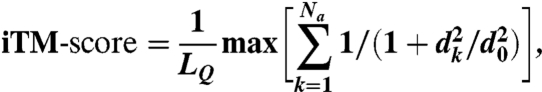
We previously introduced two scoring functions, the iTM-score and IS-score, to quantify the similarity between two aligned protein–protein interfaces (20). Although the iTM-score considers the match of backbone C_α atom geometry, the IS-score incorporates both the geometry of C_α atoms and the patterns of interfacial contacts. Given a query interface with residues i = 1…L_Q, a template interface (from a library of structures) with residues j = 1…L_T, and an alignment (k = 1…N_a) between the query and the template, the iTM-score is

[1]

where d_k is the distance in angstroms between the C_α atoms from the kth aligned residue pair, and the empirical scaling factor d₀ ≡ 1.24(L_Q - 15)^1/3 - 1.8 for a sequential alignment (29) and d₀ ≡ 0.7(L_Q - 15)^1/3 - 0.1 for nonsequential alignment. The constants in d₀ were obtained by fitting the distribution of C_α distances in random alignments to ensure that mean of scores of random interfaces is length-independent (Fig. S3). The IS-score is defined as

[2]

where

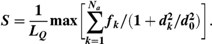[3]

Here, the contact overlap factor f_k ≡ (c_k/a_k + c_k/b_k)/2, where a_k and b_k are the numbers of interfacial contacts of the template and query interface at the kth position of the alignment, respectively, and c_k is the number of pairs of overlapping interfacial contacts at the same position. A pair of interfacial contacts overlap if the residues forming these contacts are aligned in the two pairs of chains. To make the IS-score length-independent, 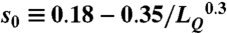is introduced (Fig. S3). For a perfect alignment between two identical structures, both the iTM-score and IS-score give the maximum score of one.

Alignment Algorithm.

Previously, we described the heuristic algorithm implemented in iAlign for finding the optimal sequential alignment between two interfaces (20). Briefly, the algorithm originally has two phases. In the first, several guessed solutions are generated by gapless alignments, secondary structure comparison, and fragment alignments. Starting from these guessed alignments, dynamic programming is iteratively applied in the second phase. Here, to identify a nonsequential alignment between two interfaces, iAlign continues to the third phase by iteratively searching for an optimal nonsequential alignment, which we have converted to the linear sum assignment problem (LSAP). To solve LSAP efficiently, we use the shortest augmenting path algorithm (30), which has a polynomial time complexity of O(N³), where N = max(L_T,L_Q). For details, see SI Methods.

Statistical Significance.

The statistical significance of IS-scores from nonsequential alignments is estimated by comparing about 1.8 million random protein–protein complex pairs and deriving an appropriate statistical model as described in SI Methods.

Library of Artificial Protein–Protein Interfaces.

From the monomeric proteins in PDB150, we chose 244 single-domain proteins with less than 300 residues and < 30% pairwise sequence identity. Using these 244 proteins as queries for the structural comparison program TM-align (25), we scanned a library of polyvaline structures previously generated with the protein structure prediction package TASSER (13). Corresponding to each query monomer, the highest TM-score–ranked polyvaline structure was selected. We name these query/polyvaline pairs as matched native/artificial monomer pairs. The mean monomer TM-score of these 244 matched monomer pairs is 0.43, which is significant but still much less than a typical TM-score > 0.5 between protein monomeric structures from the same SCOP fold. Note that we later excluded any artificial/native interface match if these interfaces are from two complexes sharing at least one of these structurally similar native/artificial monomer pairs. The selected polyvaline structures were subsequently converted to all-atom models by mutating their sequences to randomly chosen permutations of an arbitrary sequence (Escherichia coli asparagine synthetase, PDB_chain: 12as_A). From these structures, 1,756 random heteropairs and 244 homopairs are generated, totaling 2,000 pairs. For each pair, rigid-body docking is conducted with FTDock (31), and the top 2,500 docking models ranked according to shape complementarity were clustered. For each docking pair, the top 10 cluster representative protein–protein complex models were retained. Extracting interfaces from these docking models gives a total of 20,000 artificial protein–protein interfaces.

References

- 1.Nooren IMA, Thornton JM. Diversity of protein–protein interactions. EMBO J. 2003;22(14):3486–3492. doi: 10.1093/emboj/cdg359. [DOI] [PMC free article] [PubMed] [Google Scholar]
- 2.Russell RB, et al. A structural perspective on protein–protein interactions. Curr Opin Struct Biol. 2004;14:313–324. doi: 10.1016/j.sbi.2004.04.006. [DOI] [PubMed] [Google Scholar]
- 3.Janin J, Bahadur RP, Chakrabarti P. Protein–protein interaction and quaternary structure. Q Rev Biophys. 2008;41:133–180. doi: 10.1017/S0033583508004708. [DOI] [PubMed] [Google Scholar]
- 4.Jones S, Thornton JM. Principles of protein–protein interactions. Proc Natl Acad Sci USA. 1996;93:13–20. doi: 10.1073/pnas.93.1.13. [DOI] [PMC free article] [PubMed] [Google Scholar]
- 5.Keskin Z, Gursoy A, Ma B, Nussinov R. Principles of protein–protein interactions: What are the preferred ways for proteins to interact? Chem Rev. 2008;108:1225–1244. doi: 10.1021/cr040409x. [DOI] [PubMed] [Google Scholar]
- 6.Petrey D, Honig B. Is protein classification necessary? Toward alternative approaches to function annotation. Curr Opin Struct Biol. 2009;19:363–368. doi: 10.1016/j.sbi.2009.02.001. [DOI] [PMC free article] [PubMed] [Google Scholar]
- 7.Sadreyev RI, Kim BH, Grishin NV. Discrete-continuous duality of protein structure space. Curr Opin Struct Biol. 2009;19:321–328. doi: 10.1016/j.sbi.2009.04.009. [DOI] [PMC free article] [PubMed] [Google Scholar]
- 8.Valas RE, Yang S, Bourne PE. Nothing about protein structure classification makes sense except in the light of evolution. Curr Opin Struct Biol. 2009;19:329–334. doi: 10.1016/j.sbi.2009.03.011. [DOI] [PMC free article] [PubMed] [Google Scholar]
- 9.Finkelstein AV, Ptitsyn OB. Why do globular-proteins fit the limited set of folding patterns. Prog Biophys Mol Biol. 1987;50:171–190. doi: 10.1016/0079-6107(87)90013-7. [DOI] [PubMed] [Google Scholar]
- 10.Chothia C. Proteins—1000 families for the molecular biologist. Nature. 1992;357:543–544. doi: 10.1038/357543a0. [DOI] [PubMed] [Google Scholar]
- 11.Kihara D, Skolnick J. The PDB is a covering set of small protein structures. J Mol Biol. 2003;334:793–802. doi: 10.1016/j.jmb.2003.10.027. [DOI] [PubMed] [Google Scholar]
- 12.Zhang Y, Hubner IA, Arakaki AK, Shakhnovich E, Skolnick J. On the origin and highly likely completeness of single-domain protein structures. Proc Natl Acad Sci USA. 2006;103:2605–2610. doi: 10.1073/pnas.0509379103. [DOI] [PMC free article] [PubMed] [Google Scholar]
- 13.Skolnick J, Arakaki AK, Lee SY, Brylinski M. The continuity of protein structure space is an intrinsic property of proteins. Proc Natl Acad Sci USA. 2009;106:15690–15695. doi: 10.1073/pnas.0907683106. [DOI] [PMC free article] [PubMed] [Google Scholar]
- 14.Aloy P, Ceulemans H, Stark A, Russell RB. The relationship between sequence and interaction divergence in proteins. J Mol Biol. 2003;332:989–998. doi: 10.1016/j.jmb.2003.07.006. [DOI] [PubMed] [Google Scholar]
- 15.Aloy P, Russell RB. Ten thousand interactions for the molecular biologist. Nat Biotechnol. 2004;22:1317–1321. doi: 10.1038/nbt1018. [DOI] [PubMed] [Google Scholar]
- 16.Kim WK, Henschel A, Winter C, Schroeder M. The many faces of protein–protein interactions: A compendium of interface geometry. PLOS Comput Biol. 2006;2:1151–1164. doi: 10.1371/journal.pcbi.0020124. [DOI] [PMC free article] [PubMed] [Google Scholar]
- 17.Shoemaker BA, Panchenko AR, Bryant SH. Finding biologically relevant protein domain interactions: Conserved binding mode analysis. Protein Sci. 2006;15:352–361. doi: 10.1110/ps.051760806. [DOI] [PMC free article] [PubMed] [Google Scholar]
- 18.Zhang QC, Petrey D, Norel R, Honig BH. Protein interface conservation across structure space. Proc Natl Acad Sci USA. 2010;107:10896–10901. doi: 10.1073/pnas.1005894107. [DOI] [PMC free article] [PubMed] [Google Scholar]
- 19.Tsai CJ, Lin SL, Wolfson HJ, Nussinov R. A dataset of protein–protein interfaces generated with a sequence-order-independent comparison technique. J Mol Biol. 1996;260:604–620. doi: 10.1006/jmbi.1996.0424. [DOI] [PubMed] [Google Scholar]
- 20.Gao M, Skolnick J. iAlign: A method for the structural comparison of protein–protein interfaces. Bioinformatics. 2010;26:2259–2265. doi: 10.1093/bioinformatics/btq404. [DOI] [PMC free article] [PubMed] [Google Scholar]
- 21.Keskin O, Nussinov R. Similar binding sites and different partners: Implications to shared proteins in cellular pathways. Structure. 2007;15:341–354. doi: 10.1016/j.str.2007.01.007. [DOI] [PubMed] [Google Scholar]
- 22.Chen HL, Skolnick J. M-TASSER: An algorithm for protein quaternary structure prediction. Biophys J. 2008;94:918–928. doi: 10.1529/biophysj.107.114280. [DOI] [PMC free article] [PubMed] [Google Scholar]
- 23.Murzin AG, Brenner SE, Hubbard T, Chothia C. SCOP—A structural classification of proteins database for the investigation of sequences and structures. J Mol Biol. 1995;247:536–540. doi: 10.1006/jmbi.1995.0159. [DOI] [PubMed] [Google Scholar]
- 24.Altschul SF, et al. Gapped BLAST and PSI-BLAST: A new generation of protein database search programs. Nucleic Acids Res. 1997;25:3389–3402. doi: 10.1093/nar/25.17.3389. [DOI] [PMC free article] [PubMed] [Google Scholar]
- 25.Zhang Y, Skolnick J. TM-align: A protein structure alignment algorithm based on the TM-score. Nucleic Acids Res. 2005;33:2302–2309. doi: 10.1093/nar/gki524. [DOI] [PMC free article] [PubMed] [Google Scholar]
- 26.English CM, Adkins MW, Carson JJ, Churchill MEA, Tyler JK. Structural basis for the histone chaperone activity of Asf1. Cell. 2006;127:495–508. doi: 10.1016/j.cell.2006.08.047. [DOI] [PMC free article] [PubMed] [Google Scholar]
- 27.Mousson F, et al. Structural basis for the interaction of Asf1 with histone H3 and its functional implications. Proc Natl Acad Sci USA. 2005;102:5975–5980. doi: 10.1073/pnas.0500149102. [DOI] [PMC free article] [PubMed] [Google Scholar]
- 28.Uetz P, et al. A comprehensive analysis of protein–protein interactions in Saccharomyces cerevisiae. Nature. 2000;403:623–627. doi: 10.1038/35001009. [DOI] [PubMed] [Google Scholar]
- 29.Zhang Y, Skolnick J. Scoring function for automated assessment of protein structure template quality. Proteins. 2004;57:702–710. doi: 10.1002/prot.20264. [DOI] [PubMed] [Google Scholar]
- 30.Derigs U. The shortest augumenting path method for solving assignment problems—Motivation and computational experience. In: Monma CL, editor. Algorithms and Software for Optimization. Vol 4. Basel: Baltzer; 1985. pp. 57–102. [Google Scholar]
- 31.Gabb HA, Jackson RM, Sternberg MJE. Modelling protein docking using shape complementarity, electrostatics and biochemical information. J Mol Biol. 1997;272:106–120. doi: 10.1006/jmbi.1997.1203. [DOI] [PubMed] [Google Scholar]
- 32.Humphrey W, Dalke A, Schulten K. VMD: Visual molecular dynamics. J Mol Graphics. 1996;14:33–38. doi: 10.1016/0263-7855(96)00018-5. [DOI] [PubMed] [Google Scholar]
Associated Data
This section collects any data citations, data availability statements, or supplementary materials included in this article.