Analyzing effective connectivity with fMRI

Abstract

Functional neuroimaging techniques are used widely in cognitive neuroscience to investigate aspects of functional specialization and functional integration in the human brain. Functional integration can be characterized in two ways, functional connectivity and effective connectivity. While functional connectivity describes statistical dependencies between data, effective connectivity rests on a mechanistic model of the causal effects that generated the data. This review addresses the conceptual and methodological basis of established techniques for characterizing effective connectivity using functional magnetic resonance imaging (fMRI) data. In particular, we focus on dynamic causal modeling (DCM) of fMRI data and emphasize the importance of model selection procedures and nonlinear mechanisms for context-dependent changes in connection strengths.

Introduction

Functional integration in neuronal systems can be quantified in two ways, functional connectivity and effective connectivity [1-3]. While functional connectivity only describes statistical dependencies between spatially segregated neuronal events, effective connectivity rests on a mechanistic model of how the data were caused. This article reviews established techniques for characterizing effective connectivity on the basis of fMRI data, focusing on dynamic causal models (DCMs; [4, 5]).

Effective connectivity

The term effective connectivity has been defined by various authors in convergent ways. A general definition is that effective connectivity describes the causal influences that neural units exert over another [1]. More specifically, other authors have proposed that “effective connectivity should be understood as the experiment- and time-dependent, simplest possible circuit diagram that would replicate the observed timing relationships between the recorded neurons” [6]. Both definitions emphasize that determining effective connectivity requires a causal model of the interactions between the elements of the neural system of interest.

Such causal models can be defined within the general mathematical framework provided by dynamic systems theory [7-9]. A system is characterised by time-variant properties x_i (1 ≤ i ≤ n) or state variables, which interact with each other, i.e. the evolution of each state variable depends on at least one other state variable. For example, the postsynaptic membrane potential depends on which and how many ion channels are open; vice versa, the probability of voltage-dependent ion channels opening depends on the membrane potential. Such functional dependencies can be expressed quite naturally by a set of ordinary differential equations in which a set of parameters θ determine the form and strength of the causal influences between the state variables. In neural systems, these parameters usually include time constants or synaptic strengths of the connections between the system elements. Additionally, in the case of non-autonomous systems (i.e. systems that exchange matter, energy or information with their environment) we need to consider the inputs into the system, e.g. sensory information entering the brain. Representing the set of all m known inputs by the m-vector function u(t), one can define a general state equation for non-autonomous deterministic systems:

$$\frac{\mathit{dx}}{\mathit{dt}}=F(x,u,\theta )$$ (1)

A model whose form follows this general state equation provides a causal description of how system dynamics results from system structure, because it describes (i) when and where external inputs enter the system and (ii) how the state changes induced by these inputs evolve in time depending on the system's structure. Given a particular temporal sequence of inputs u(t) and an initial state x(0), one obtains a complete description of how the dynamics of the system (i.e. the trajectory of its state vector x in time) results from its structure by integration of Equation 1:

$$x\left(\tau \right)=x\left(0\right)+\underset{0}{\overset{\tau }{\int }}F(x,u,\theta )\mathit{dt}$$ (2)

Equation 2 therefore provides a general form for models of effective connectivity in neural systems. (It assumes that all processes in the system are deterministic and occur instantaneously, but can easily be extended, e.g. by using stochastic and delay differential equations, respectively [10, 11]). The framework outlined here is concerned with dynamic systems in continuous time and thus uses differential equations. The same basic ideas, however, can also be applied to dynamic systems in discrete time (using difference equations), e.g. multivariate/vector autoregressive models (MAR/VAR; [12-14], as well as to “static” systems where the system is at equilibrium at each point of observation. The latter perspective applies to regression-based system models for functional neuroimaging data, e.g. psycho-physiological interactions (PPI; [15]), or structural equation modeling (SEM; [16-19]). Readers interested in these classical approaches are referred to the original articles referenced above and to reviews that have compared these approaches (e.g. [7, 20]). Here, we focus on that framework for inferring effective connectivity from fMRI data that most closely follows Equation 2 above, i.e. dynamic causal modeling ([4, 5]).

Dynamic Causal Modelling (DCM)

An important limitation of classical models of effective connectivity like PPI, SEM or VAR is that they operate at the level of the measured signals. This is a serious problem because the causal architecture of the system that we would like to identify is located at the neuronal level which cannot be investigated directly using non-invasive techniques. In the case of fMRI data, for example, PPI, SEM and VAR are fitted to measured time series which result from a haemodynamic convolution of the underlying neuronal activity. The absence of a forward model linking neuronal activity to the measured haemodynamic data can render analyses of inter-regional connectivity problematic. For example, different brain regions can exhibit marked differences in neurovascular coupling. It has been shown that these inter-regional differences can lead to false inference about effective connectivity [21]. A similar problem exists for EEG data where changes in neural activity in different brain regions lead to changes in electric potentials that superimpose linearly. The scalp electrodes therefore record a mixture, with unknown weightings, of potentials generated by a number of different sources.

Therefore, to enable inferences about connectivity between neural units we need models that combine two things: (i) a parsimonious but neurobiologically plausible model of neural population dynamics, and (ii) a biophysically plausible forward model that describes the transformation from neural activity to the measured signal (c.f. [13, 22]). Such models make it possible to fit jointly the parameters of the neural and of the forward model such that the predicted time series are optimally similar to the observed time series. In principle, any of the models described above could be combined with a modality-specific forward model, and indeed, VAR models have previously been combined with linear forward models to explain EEG data [23]. So far, however, DCM is the only approach where the marriage between models of neural dynamics and biophysical forward models is a mandatory component.

Since its original inception for fMRI [4], a variety of DCM implementations have been introduced for additional data modalities, including event-related potentials [11, 24] induced responses [25, 26], auto- and cross-spectral densities [27, 28] and phase coupling [29] as measured by local field potential recordings or EEG/MEG. These models, all formulated under the same theoretical framework, have enjoyed considerable success in the practical analysis of neuroimaging data, resulting in more than 100 published studies (as of August 2009). In this chapter, we focus on DCM for fMRI as originally described [4] and on some recent nonlinear extensions of this model [30].

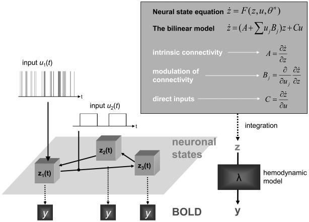
DCM for fMRI uses a simple model of neural dynamics in a system of n interacting brain regions (see Figure 1 for a schematic summary). In its classical form [4], it models the change of a neural state vector x in time, with each region in the system being represented by a single state variable (representing mean regional activity), using the following bilinear differential equation:

$$\begin{array}{cc}\hfill \frac{\mathit{dx}}{\mathit{dt}}& =F\left(x,u,{\theta }^n\right)\hfill \\ \hfill & =\left(A+\underset{i=1}{\overset{m}{\Sigma }}{u}_j{B}^{\left(i\right)}\right)x+\mathit{Cu}\hfill \end{array}$$ (3)

Note that this neural state equation follows the general form for deterministic system models introduced by Equation 2, i.e. the modelled state changes are a function of the system state itself, the inputs u and some parameters θ⁽ⁿ⁾ that define the functional architecture and interactions among brain regions at a neuronal level. The neural state variables represent a summary index of neural population dynamics in the respective regions. The neural dynamics are driven by experimentally controlled external inputs that can enter the model in two different ways: they can elicit responses through direct influences on specific regions (e.g. evoked responses in early sensory cortices; the C matrix) or they can modulate the coupling among regions (e.g. during learning or attention; the B matrices). Note that Eq. 3 does not account for conduction delays in either inputs or inter-regional influences. This is not necessary because, due to the large regional variability in hemodynamic response latencies, fMRI data do not posses enough temporal information to enable estimation of inter-regional axonal conduction delays which are typically in the order of 10-20 ms (note that the differential latencies of the hemodynamic response are accommodated by region-specific biophysical parameters in the hemodynamic model described below). This was verified by Friston et al. [4] who showed in simulations that DCM parameter estimates were not affected by introducing artificial delays of up to ± 1 second. In contrast, conduction delays are an important part of DCM for event-related potentials [11].

Figure 1.

Schematic summary of the conceptual basis of DCM. The dynamics in a system of interacting neuronal populations (left lower panel), which are not directly observable by fMRI, is modeled using a bilinear state equation (right upper panel). Integrating the state equation gives predicted neural dynamics (z) that enter a model of the hemodynamic response (λ) to give predicted BOLD responses (y) (right lower panel). The parameters at both neural and hemodynamic levels are adjusted such that the differences between predicted and measured BOLD series are minimized. Critically, the neural dynamics are determined by experimental manipulations. These enter the model in the form of external inputs (left upper panel). Driving inputs (u₁; e.g. sensory stimuli) elicit local responses directly that are propagated through the system according to the intrinsic connections. The strengths of these connections can be changed by modulatory inputs (u₂; e.g. changes in cognitive set, attention, or learning). In this figure, the structure of the system and the scaling of the inputs are arbitrary. This figure was reproduced, with permission, from Figure 1 in [36].

Given the bilinear state equation (Equation 3), the neural parameters θ⁽ⁿ⁾ = {A, B, C} can be expressed as partial derivatives of F:

$$\begin{array}{cc}\hfill & A={\phantom{\mid }\frac{\partial F}{\partial x}\mid }_{u=0}\hfill \\ \\ \hfill & B^{\left(i\right)}=\frac{{\partial }^{2}F}{\partial x\partial u_i}\hfill \\ \\ \hfill & C={\phantom{\mid }\frac{\partial F}{\partial u}\mid }_{x=0}\hfill \end{array}$$ (4)

As can be seen from these equations, the matrix A represents the endogenous (fixed) connectivity among the regions in the absence of input, the matrices B⁽ⁱ⁾ encode the change in connectivity induced by the i^th input u_i, and C embodies the strength of exogenous (direct) influences of inputs on neuronal activity. In most instances, the parameters of primary interest are the modulatory ones (i.e. the matrices B⁽ⁱ⁾) since they encode how experimentally controlled manipulations change the connection strengths in the system.

DCM for fMRI combines this model of neural dynamics with an experimentally validated haemodynamic model that describes the transformation of neuronal activity into a BOLD response. This haemodynamic model, which builds on the so-called “Balloon model” [31], consists of a set of differential equations that describe, using a set of parameters θ^(h), how changes in neural activity elicit changes in a vasodilatory signal, blood flow, blood volume and deoxyhemoglobin content [32]. The predicted BOLD signal is a non-linear function of blood volume and deoxyhemoglobin content [33]. The most recent version of this haemodynamic model is summarised by Figure 2 and described in detail by Stephan et al. [33].

Figure 2.

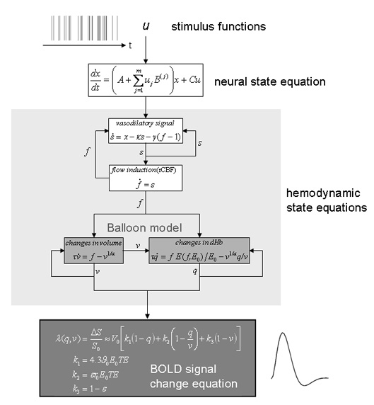
Schematic summary of the neural state equation and the hemodynamic forward model in DCM; reproduced, with permission, from Figure 1 in [33]. Experimentally controlled input functions u evoke neural responses x, modeled by a bilinear differential state equation, which trigger a hemodynamic cascade, modeled by 4 state equations with 5 parameters. These hemodynamic parameters comprise the rate constant of the vasodilatory signal decay (κ), the rate constant for auto-regulatory feedback by blood flow (γ), transit time (τ), Grubb's vessel stiffness exponent (α), and capillary resting net oxygen extraction (ρ). The so-called Balloon model consists of the two equations describing the dynamics of blood volume (v) and deoxyhemoglobin content (q) (light grey boxes). Integrating the state equations for a given set of inputs and parameters produces predicted time-series for v and q which enter a BOLD signal equation λ (dark grey box) to give a predicted BOLD response.

The combined neural and haemodynamic parameter set θ = {θ⁽ⁿ⁾, θ⁽ⁿ⁾} is estimated from the measured BOLD data, using a fully Bayesian approach with empirical priors for the haemodynamic parameters and conservative shrinkage priors for the coupling parameters. Details of the parameter estimation scheme, which rests on a fixed-form variational Bayesian algorithm, using a Laplace (i.e. Gaussian) approximation to the true posterior, can be found elsewhere [4, 34, 35].

Inference about neuronal mechanisms with DCM

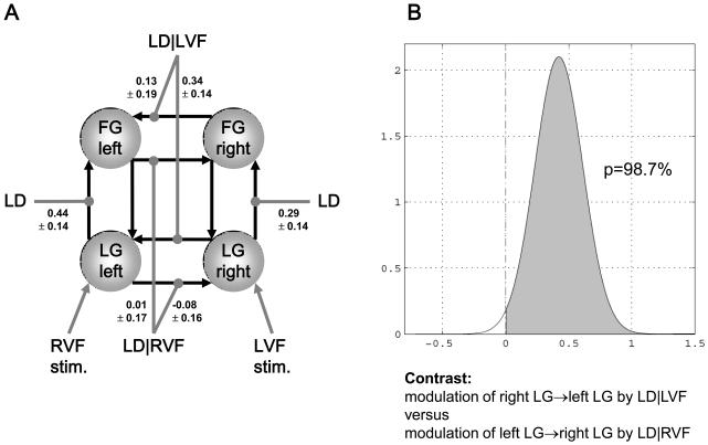
Once the parameters of a DCM have been estimated from measured BOLD data, the posterior distributions of the parameter estimates can be used to test hypotheses about connection strengths. Due to the Laplace approximation, the posterior distributions are defined by their maximum a posteriori (MAP) estimate and their posterior covariance. Usually, the hypotheses to be tested concern context-dependent changes in coupling (i.e. the matrices B⁽ⁱ⁾ in Eq. 3). An example, originally reported in [36], is given by Figure 3. Here, DCM was applied to fMRI data from a single subject, testing the hypothesis that in the ventral stream of the visual system a letter decision task increased the strength of interhemispheric connections, but only when the word stimuli were presented in the left visual field and were thus initially received by the non-dominant right hemisphere, necessitating transfer of stimulus information to the specialised left hemisphere. This hypothesis was tested by constructing a four-area model of ventral stream areas, comprising the lingual and fusiform gyri in both hemispheres (Figure 3A), and comparing the modulatory influences of task, conditional on the visual field of stimulus presentation, for interhemispheric connections in both directions. This comparison, based on the MAP estimates and the posterior covariances of the modulatory parameters, indicated that for this particular subject and for the connections between left and right lingual gyrus the hypothesised asymmetry in interhemispheric transfer existed with a probability of 98.7% (Figure 3B). Other examples of single-subject analyses can be found in [4, 20, 30, 37].

Figure 3.

This figure was adapted, with permission, from Figures 5 and 6 in [36]. It shows an example of a single subject DCM that was used to study asymmetries in interhemispheric connections during a letter decision task. LG = lingual gyrus, FG = fusiform gyrus, LD = letter decisions, LD|VF = letter decisions conditional on the visual field of stimulus presentation.

A. The values denote the maximum a posteriori (MAP) estimates of the parameters (± square root of the posterior variances; units: 1/s=Hz). For clarity, only the parameters of interest, i.e. the modulatory parameters of inter- and intra-hemispheric connections, are shown.

B. Asymmetry of callosal connections with regard to contextual modulation. The plots show the probability (98.7%) that the modulation of the right LG → left LG connection is stronger than the modulation of the left LG → right LG connection.

For statistical inference at the group level, various options exist. One commonly used approach, corresponding to a random effects analysis, is to enter the conditional estimates of interest into a classical second-level analysis, e.g. a t-test on the MAP estimates of a particular parameter across subjects (for examples, see [38-41]). An alternative approach is to use Bayesian statistics at the group level as well. This can be done by computing, for a given parameter, one joint posterior density across all subjects, treating the posterior of one subject as the prior for the next [42]. This approach can be more sensitive; its disadvantage, however, is that it corresponds to a fixed effects analysis and thus does not allow for inference beyond the particular group studied.

Bayesian model selection (BMS)

Model comparison and selection is central to the scientific process, in that it allows one to evaluate different hypotheses about the way data are caused [43, 44]. Nearly all scientific reporting rests upon some form of model comparison, which represents a probabilistic statement about the beliefs in one hypothesis relative to some other(s), given some observations or data. In other words: Given some observed data, which of several alternative models is optimal? The decision cannot be made solely by comparing the relative fit of competing models. One also needs to account for differences in complexity; i.e., the number of free parameters and the degree of their inter-dependency. This is important because as model complexity increases, fit increases monotonically, but at some point the model will start fitting noise that is specific to the particular data (i.e., “over-fitting”) and thus becomes less generalizable across multiple realizations of the same underlying generative process. Therefore, the question “What is the optimal model?” can be reformulated as “What is the model that represents the best balance between fit and complexity?” This is the model that maximizes the model evidence:

$$p(y\mid m)=\int p(y\mid \theta ,m)p(\theta \mid m)d\theta$$ (5)

Here, the numbers of free parameters (as well as the functional form of the generative model that determines their interdependencies) are subsumed by the integration. Unfortunately, this integral cannot usually be solved analytically; therefore an approximation to the (log of the) model evidence is used instead. This approximation is usually a free energy bound on the log evidence [35]; alternatively, simpler criteria like the Akaike Information Criterion [45] or the Bayesian Information Criterion [46] can be used that are blind to parameter interdependencies (see [47] for a detailed discussion). Given any of these approximations to the log evidence of two models m_i and m_j, the difference in log evidence can be transformed into a Bayes factor (BF):

$${\mathit{BF}}_{\mathit{ij}}=\frac{p(y\mid m_i)}{p(y\mid m_i)}\approx \exp (F_i-F_j)$$ (6)

BMS can be applied both to single subjects and whole groups. When the optimal model structure is expected to vary across subjects (e.g., subject-specific cognitive strategies or different pathophysiological mechanisms in a group of patients), random effects BMS is required. This method rests on a hierarchical model which is optimised to furnish a probability density on the models themselves, using variational Bayes [47]. Specifically, it estimates the parameters of a Dirichlet distribution describing the probabilities for all models considered. These probabilities then define a multinomial distribution over model space, allowing one to compute how likely it is that a specific model generated the data of a randomly chosen subject as well as the exceedance probability of one model being more likely than any other model.

BMS plays a central role for DCM. It is used routinely to select the most likely model amongst a set of alternatives before making inferences about particular parameters, e.g., [33, 38, 42, 48-54]. An alternative use of model selection is to decide about the nature of particular mechanisms without the need for any further inference about particular parameters. For example, BMS has been used to compare DCMs with non-linear versus linear BOLD equations in the haemodynamic forward model [33, 47] or to disambiguate between different possibilities how anatomical connection strength constrains effective connection strength [55]. A particularly interesting approach is to go beyond the comparison of specific models and compare two (or more) partitions of model space [47]. These partitions would typically reflect those components of model structure that one seeks inference about, e.g. whether a specific connection should be included in the model or not, whether a particular connection is modulated by one experimental condition or another, or whether certain effects are linear or nonlinear. The advantage of this method is that arbitrarily large set of models can be considered together, allowing one to integrate out uncertainty over any aspect of model structure other than the component of interest.

Nonlinear DCM for fMRI

Since its first description [4], DCM for fMRI has been extended in several ways. For example, an extension of the observation equation takes into account the slice-specific sampling times in multi-slice MRI acquisitions [56]. This enables DCM to be applied to fMRI data from any data acquisition scheme. Another variant represents each region in the model by two state variables and distinguishes between population activity of excitatory and inhibitory neurons [57]. Other work has augmented DCM with a spatial model of the regional time series to which the model is fitted [58].

Here, we focus on what we consider to be a particularly important extension of DCM for fMRI, namely the inclusion of nonlinear modulatory effects [30]. This extension was motivated by two limitations of the original bilinear neuronal state equation in DCM. First, the neuronal origin of the modulatory influence is not specified. Second, the bilinear framework may not be the most appropriate choice for modelling fast changes in effective connectivity, which are mediated by nonlinear effects at the level of single neurons. These mechanisms are instances of “short-term synaptic plasticity” (STP), an umbrella term for a range of processes which alter synaptic strengths with time constants in the range of milliseconds to minutes; e.g. NMDA-controlled rapid trafficking or phosphorylation of AMPA receptors, synaptic depression/facilitation or “early LTP”. All these processes are driven by the history of prior synaptic activity and are thus nonlinear [59].

A particularly interesting mechanism, which relies on STP, is “neuronal gain control”. Neuronal gain, i.e. the response of a given neuron N₁ to presynaptic input from a second neuron N_2, depends on the history of inputs that N₁ receives from other neurons, e.g. a third neuron N₃. Such a nonlinear modulation or “gating” of the N₂→ N₁ connection by N₃ has been shown to have the same mathematical form across a large number of experiments (for review, see [60]): the change in the gain of N₁ results from a multiplicative interaction among the synaptic inputs from N₂ and N₃, i.e. a second-order nonlinear effect. Biophysically, neuronal gain control can arise through various mechanisms that mediate interactions among synaptic inputs occurring close in time (see [30] for a discussion of these mechanisms).

Critically, the bilinear framework precludes a representation, at the neuronal level, of the mechanisms described above. As stated in the original DCM paper [4], in order to model processes like neuronal gain control and synaptic plasticity properly, one needs “to go beyond bilinear approximations to allow for interactions among the states. This is important when trying to model modulatory or nonlinear connections such as those mediated by backward afferents that terminate predominantly in the supragranular layers and possibly on NMDA receptors.”

Therefore, to enable a realistic representation of how neuronal populations modulate the gains of other populations, one needs to model nonlinear interactions amongst the n states of a given DCM. For this purpose, one can use a two-dimensional Taylor series which is of second order in the states [30]:

$$\begin{array}{cc}\hfill & f(x,u)=\frac{\mathit{dx}}{\mathit{dt}}\hfill \\ \hfill & \approx f(0,0)+\frac{\partial f}{\partial x}x+\frac{\partial f}{\partial u}u+\frac{{\partial }^{2}f}{\partial x\partial u}\mathit{xu}+\frac{{\partial }^{2}f}{\partial x^2}\frac{x^2}{2}\hfill \end{array}$$ (7)

Setting $D^{\left(j\right)}={\phantom{\mid }\frac{1}{2}\frac{{\partial }^{2}f}{\partial x_j^2}\mid }_{u=0}(1\le j\le n)$ makes Eq. 7 equivalent to:

$$f(x,u)=\frac{\mathit{dx}}{\mathit{dt}}=\left(A+\underset{i=1}{\overset{m}{\Sigma }}{u}_i{B}^{\left(i\right)}+\underset{j=1}{\overset{n}{\Sigma }}{x}_j{D}^{\left(j\right)}\right)x+\mathit{Cu}$$ (8)

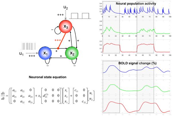
Here, the D^(j) matrices encode which of the n regions gate which connections in the system. Specifically, any non-zero entry $D_{\mathit{kl}}^{\left(j\right)}$ indicates that responses of region k to inputs from region l depend on activity in region j. Figure 4 shows a simple example, with synthetic data generated by a nonlinear DCM. This illustrates the sort of dynamics, both at the neuronal and hemodynamic level which this sort of model exhibits.

Figure 4.

An example of the neuronal and haemodynamic dynamics that can be accounted for by nonlinear DCMs. The figure is reproduced, with permission, from Figure 2 in [30]. The right panel shows synthetic neuronal and BOLD time-series that were generated using the nonlinear DCM shown on the left. In this model, neuronal population activity x₁ (blue) is driven by irregularly spaced random events (delta-functions). Activity in x₂ (green) is driven through a connection from x₁; critically, the strength of this connection depends on activity in a third population, x₃ (red), which receives a connection from x₂ but also receives a direct input from a box-car input. The effect of nonlinear modulation can be seen easily: responses of x₂ to x₁ become negligible when x₃ activity is low. Conversely, x₂ responds vigorously to x₁ inputs when the x₁→x₂ connection is gated by x₃ activity. Strengths of connections are indicated by symbols (−: negative; +: weakly positive; +++: strongly positive).

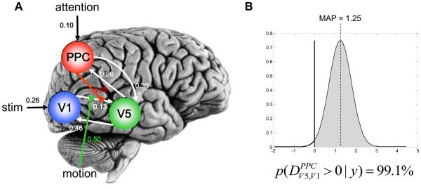
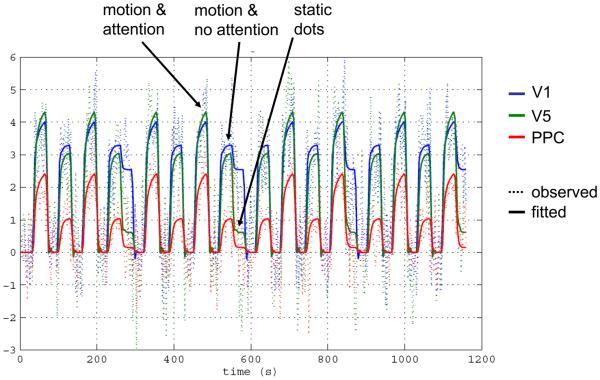
The nonlinear extension enhances the kind of dynamics that DCM can capture and enables the user to implement additional types of models. Beyond modelling how connection strengths are modulated by external inputs, one can now model how connection strengths are gated by the activity of one or several neuronal populations. This ability is critical for various applications, e.g. for marrying reinforcement learning models with DCM [7], but also for mechanistic accounts of the effects of attention. For example, nonlinear DCM was applied to a single-subject data set from a blocked fMRI study of attention to visual motion [17]. Four different models were compared [30], each of which embodied a different explanation for the empirical finding that V5 responses increased during attention to motion, compared to unattended motion. The most likely model was one in which the gain of the V1→V5 connection depended on the activity in the posterior parietal cortex (PPC), a region on which attention exerted a direct effect (this could result, for example, from cholinergic inputs from the brainstem [61]). Analysis of the posterior density of the modulatory parameter in this model indicated that nonlinear gating of the V1→V5 connection by attention could be inferred with 99.1% confidence (see Figure 5). Figure 6 shows the observed and fitted time-series of all areas and highlights the attentional gating effect on V5 activity, such that V5 activity was higher when subjects attended the moving stimuli.

Figure 5.

Application of nonlinear DCM to single subject fMRI data from an attention to motion paradigm [17]. The figure is reproduced, with permission, from Figure 7 in [30].

A. Maximum a posteriori estimates of all parameters. PPC = posterior parietal cortex.

B. Posterior density of the estimate for the nonlinear modulation parameter for the V1→V5 connection. Given the mean and variance of this posterior density, we have 99.1% confidence that the true parameter value is larger than zero or, in other words, that there is an increase in gain of V5 responses to V1 inputs that is mediated by PPC activity.

Figure 6.

Fit of the nonlinear model to the attention to motion data in Figure 5. Dotted lines represent the observed data, solid lines the responses predicted by the nonlinear DCM. The increase in the gain of V5 responses to V1 inputs during attention is clearly visible. The figure is reproduced, with permission, from Figure 8 in [30].

As a second example for the practical utility of nonlinear DCMs, we show the results from a single subject analysis of fMRI data set acquired during an event-related binocular rivalry paradigm [30]. While there is no clear consensus about the mechanisms that underlie binocular rivalry, it has been suggested that it (i) depends on nonlinear mechanisms and (ii) may arise from modulation of connections amongst neuronal representations of the competing stimuli by feedback connections from higher areas [62].

The fMRI data were acquired during a factorial paradigm in which face and house stimuli were presented either during binocular rivalry or during a matched non-rivalry (i.e. replay) condition. For the subject studied here, the conventional SPM analysis showed a rivalry × percept interaction in both the right fusiform face area (FFA) and the right parahippocampal place area (PPA): in FFA, the face vs. house contrast was higher during non-rivalry than during rivalry; conversely, in PPA the house vs. face contrast was higher during non-rivalry than during rivalry (both p<0.05, small-volume corrected). Additionally, testing for a main effect of rivalry, we replicated previous findings that the right middle frontal gyrus (MFG) showed higher activity during rivalry than during non-rivalry conditions [63].

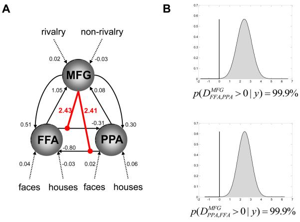
These SPM results motivated a nonlinear DCM in which the connections between FFA and PPA were modulated by the activity in the MFG (Figure 7). First, the fixed (endogenous) connection strengths between FFA and PPA were negative in both directions, i.e. FFA and PPA exerted a mutual negative influence on each other; this could be regarded as a “tonic” or “baseline” reciprocal inhibition. More importantly, however, was that during the presentation of visual stimuli this competitive interaction between FFA and PPA was modulated by activity in the middle frontal gyrus (MFG), which showed higher activity during rivalry vs. non-rivalry conditions. As shown in Figure 7, our confidence about the presence of this nonlinear modulation was very high (99.9%) for both connections.

Figure 7.

Application of nonlinear DCM to single subject fMRI data from a binocular rivalry paradigm. The figure is reproduced, with permission, from Figure 9 in [30].

A. The structure of the nonlinear DCM fitted to the binocular rivalry data, along with the maximum a posteriori estimates of all parameters. The intrinsic connections between FFA and PPA are negative in both directions; i.e. FFA and PPA mutually inhibited each other. This may be seen as an expression, at the neurophysiological level, of the perceptual competition between the face and house stimuli. This competitive interaction between FFA and PPA is modulated nonlinearly by activity in the middle frontal gyrus (MFG), which showed higher activity during rivalry vs. non-rivalry conditions.

B. Our confidence about the presence of this nonlinear modulation is very high (99.9%), for both connections.

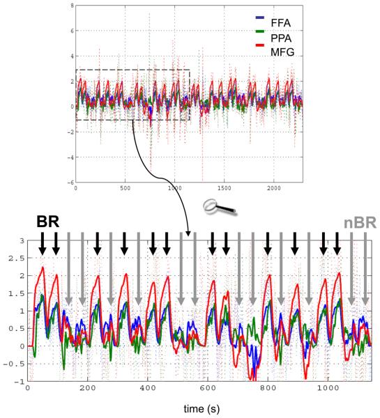
According to this model, activity levels in the MFG determine activity in FFA and PPA by controlling the influence that face-elicited activations and house-elicited deactivations of FFA have on PPA (and vice versa). For example, the positive nonlinear modulation of the FFA→PPA connection by MFG activity (see Figure 7) means that during face-perception under rivalry conditions (which elicit positive activity in the FFA and MFG, respectively) there is a positive influence of FFA on PPA, overriding the “baseline” inhibition. This means that during binocular rivalry FFA and PPA become more tightly coupled which destroys their stimulus selectivity: their activity becomes very similar, regardless of whether a face or a house is being perceived. In contrast, deactivation of MFG during non-rivalry conditions decreases the influence that FFA has on PPA during house perception; therefore responses in FFA and PPA become less coupled and their relative selectivity for face and house percepts is restored. This dynamic coupling and uncoupling, leading to less selectivity of FFA and PPA during rivalry and higher selectivity during non-rivalry, is clearly visible in Figure 8 which plots the observed and fitted responses of all three areas. Here, the short black arrows indicate blocks with binocular rivalry (when FFA and PPA show very similar time courses) and the long grey arrows denote non-rivalry blocks (when FFA and PPA activities evolve more independently). These changes in effective connectivity over time, which are controlled by the activity level in MFG, provide a nice explanation for the rivalry × percept interaction in FFA and PPA that was identified by the SPM analysis.

Figure 8.

Fit of the nonlinear model in Figure 7 to the binocular rivalry data. Dotted lines represent the observed data, solid lines the responses predicted by the nonlinear DCM. The upper panel shows the entire time series. The lower panel zooms in on the first half of the data (dotted box). One can see that the functional coupling between FFA (blue) and PPA (green) depends on the activity level in MFG (red): when MFG activity is high during binocular rivalry blocks (BR; short black arrows), FFA and PPA are strongly coupled and their responses are difficult to disambiguate. In contrast, when MFG activity is low, during non-rivalry blocks (nBR; long grey arrows), FFA and PPA are less coupled, and their activities evolve more independently. The figure is reproduced, with permission, from Figure 10 in [30].

Conclusions

In this short review, we have outlined how effective connectivity can be inferred from fMRI data using DCM. We expect that two application domains for DCM will prove to be particularly exciting and fruitful in the near future. The first domain is the integration of the neurophysiological and computational aspects of learning and decision making. For example, according to theoretical models of learning, the size of prediction errors should control synaptic plasticity, i.e. changes in the strength of synaptic connections, encoding stimulus-stimulus and stimulus-response links [64-66]. In other words, the necessity of reconfiguring neuronal circuits during learning should be inversely proportional to how well those neuronal circuits are capable of predicting sensory stimuli or outcomes of actions. This notion can be tested formally by embedding prediction errors provided by computational models of learning (such as Rescorla-Wagner or temporal difference learning models) into DCMs. A first demonstration of this approach was given by a recent study which combined DCM with a Rescorla-Wagner model and showed that during incidental audio-visual associative learning the plasticity of connections from auditory to visual cortex depended on trial-by-trial prediction errors [67]. A subsequent study extended this finding: combining nonlinear DCM and a hierarchical Bayesian learner, it showed that the degree of trial-by-trial prediction error activity in the putamen controlled the efficacy of visuomotor connections, thus gating the transfer of sensory information depending on how unexpected this information was (den Ouden et al., submitted).

The second application domain concerns the development of DCMs with clinical utility, for example as diagnostic tools. Although DCM has already been applied to some clinical questions (e.g., [39, 68, 69], the critical challenge for the future will be to develop DCMs whose parameter estimates have sufficient sensitivity and specificity to delineate subgroups of patients that are characterized by different pathophysiological mechanisms. This generic framework of model-based inference about pathophysiological processes that cannot be measured directly is likely to be particularly helpful for vaguely defined spectrum diseases. For example, our own work focuses on schizophrenia, trying to establish DCMs, in conjunction with pharmacological challenges and learning paradigms, that can detect specific abnormalities in the regulation of NMDA-dependent synaptic plasticity by neuromodulatory transmitters like dopamine or acetylcholine [70]. Hopefully, neurocomputational models of specific learning and decision-making processes (such as the work by den Ouden et al. described above) can be established whose parameters map onto well-defined physiological mechanisms of synaptic plasticity and neuromodulation. These models are not restricted to fMRI, but will also exploit electrophysiological measurements. Careful validation of these models is crucial and will require pharmacological and invasive recording studies in animals. For example, a recent rodent study demonstrated that DCM can correctly infer experimentally induced changes in spike frequency adaptation and postsynaptic efficacy of glutamatergic synapses [27].

Importantly, however, model-based inference on pathophysiology and disease status cannot only proceed on the basis of neurophysiologically interpretable parameter estimates, but could also employ BMS to compare entire models embodying different putative disease mechanisms. This inference on model structure could be particularly useful when disease subgroups differ along more than one pathophysiological dimension.

References

- 1.Friston KJ. Functional and effective connectivity in neuroimaging: a synthesis. Hum. Brain Mapp. 1994;2:56–78. [Google Scholar]
- 2.Horwitz B, Tagamets MA, McIntosh AR. Neural modeling, functional brain imaging, and cognition. Trends Cogn Sci. 1999 Mar;3(no. 3):91–98. doi: 10.1016/s1364-6613(99)01282-6. [DOI] [PubMed] [Google Scholar]
- 3.Stephan KE, Riera JJ, Deco G, Horwitz B. The Brain Connectivity Workshops: moving the frontiers of computational systems neuroscience. Neuroimage. 2008 Aug 1;42(no. 1):1–9. doi: 10.1016/j.neuroimage.2008.04.167. [DOI] [PMC free article] [PubMed] [Google Scholar]
- 4.Friston KJ, Harrison L, Penny W. Dynamic causal modelling. Neuroimage. 2003 Aug;19(no. 4):1273–302. doi: 10.1016/s1053-8119(03)00202-7. [DOI] [PubMed] [Google Scholar]
- 5.Stephan KE, Harrison LM, Kiebel SJ, David O, Penny WD, Friston KJ. Dynamic causal models of neural system dynamics:current state and future extensions. J Biosci. 2007 Jan;32(no. 1):129–44. doi: 10.1007/s12038-007-0012-5. [DOI] [PMC free article] [PubMed] [Google Scholar]
- 6.Aertsen A, Preißl H. Dynamics of activity and connectivity in physiological neuronal networks. In: HG S, editor. Nonlinear Dynamics and Neuronal Networks. VCH Publishers; New York: 1999. pp. 281–302. [Google Scholar]
- 7.Stephan KE. On the role of general system theory for functional neuroimaging. J Anat. 2004 Dec;205(no. 6):443–70. doi: 10.1111/j.0021-8782.2004.00359.x. [DOI] [PMC free article] [PubMed] [Google Scholar]
- 8.Jirsa VK. Connectivity and dynamics of neural information processing. Neuroinformatics. 2004 Sum;2(no. 2):183–204. doi: 10.1385/NI:2:2:183. [DOI] [PubMed] [Google Scholar]
- 9.Breakspear M. “Dynamic” connectivity in neural systems: theoretical and empirical considerations. Neuroinformatics. 2004;2(no. 2):205–26. doi: 10.1385/NI:2:2:205. [DOI] [PubMed] [Google Scholar]
- 10.Friston KJ, Trujillo-Barreto N, Daunizeau J. DEM: a variational treatment of dynamic systems. Neuroimage. 2008 Jul 1;41(no. 3):849–85. doi: 10.1016/j.neuroimage.2008.02.054. [DOI] [PubMed] [Google Scholar]
- 11.David O, Kiebel SJ, Harrison LM, Mattout J, Kilner JM, Friston KJ. Dynamic causal modeling of evoked responses in EEG and MEG. Neuroimage. 2006 May 1;30(no. 4):1255–72. doi: 10.1016/j.neuroimage.2005.10.045. [DOI] [PubMed] [Google Scholar]
- 12.Harrison L, Penny WD, Friston K. Multivariate autoregressive modeling of fMRI time series. Neuroimage. 2003 Aug;19(no. 4):1477–91. doi: 10.1016/s1053-8119(03)00160-5. [DOI] [PubMed] [Google Scholar]
- 13.Goebel R, Roebroeck A, Kim DS, Formisano E. Investigating directed cortical interactions in time-resolved fMRI data using vector autoregressive modeling and Granger causality mapping. Magn Reson Imaging. 2003 Dec;21(no. 10):1251–61. doi: 10.1016/j.mri.2003.08.026. [DOI] [PubMed] [Google Scholar]
- 14.Roebroeck A, Formisano E, Goebel R. Mapping directed influence over the brain using Granger causality and fMRI. Neuroimage. 2005 Mar;25(no. 1):230–42. doi: 10.1016/j.neuroimage.2004.11.017. [DOI] [PubMed] [Google Scholar]
- 15.Friston KJ, Buechel C, Fink GR, Morris J, Rolls E, Dolan RJ. Psychophysiological and modulatory interactions in neuroimaging. Neuroimage. 1997 Oct;6(no. 3):218–29. doi: 10.1006/nimg.1997.0291. [DOI] [PubMed] [Google Scholar]
- 16.McIntosh AR, Gonzalez-Lima F. Structural modeling of functional neural pathways mapped with 2-deoxyglucose: effects of acoustic startle habituation on the auditory system. Brain Res. 1991 May 3;547(no. 2):295–302. doi: 10.1016/0006-8993(91)90974-z. [DOI] [PubMed] [Google Scholar]
- 17.Büchel C, Friston KJ. Modulation of connectivity in visual pathways by attention: cortical interactions evaluated with structural equation modelling and fMRI. Cereb Cortex. 1997;7(no. 8):768–78. doi: 10.1093/cercor/7.8.768. [DOI] [PubMed] [Google Scholar]
- 18.Bullmore E, Horwitz B, Honey G, Brammer M, Williams S, Sharma T. How good is good enough in path analysis of fMRI data? Neuroimage. 2000 Apr;11(no. 4):289–301. doi: 10.1006/nimg.2000.0544. [DOI] [PubMed] [Google Scholar]
- 19.McIntosh AR, Gonzales-Lima F. Structural equation modelling and its application to network analysis in functional brain imaging. Hum Brain Mapp. 1994;2:2–22. [Google Scholar]
- 20.Penny WD, Stephan KE, Mechelli A, Friston KJ. Modelling functional integration: a comparison of structural equation and dynamic causal models. Neuroimage. 2004;23(Suppl 1):S264–74. doi: 10.1016/j.neuroimage.2004.07.041. [DOI] [PubMed] [Google Scholar]
- 21.David O, Guillemain I, Saillet S, Reyt S, Deransart C, Segebarth C, Depaulis A. Identifying neural drivers with functional MRI: an electrophysiological validation. PLoS Biol. 2008 Dec 23;6(no. 12):2683–97. doi: 10.1371/journal.pbio.0060315. [DOI] [PMC free article] [PubMed] [Google Scholar]
- 22.Stephan KE, Harrison LM, Penny WD, Friston KJ. Biophysical models of fMRI responses. Curr Opin Neurobiol. 2004 Oct;14(no. 5):629–35. doi: 10.1016/j.conb.2004.08.006. [DOI] [PubMed] [Google Scholar]
- 23.Yamashita O, Galka A, Ozaki T, Biscay R, Valdes-Sosa P. Recursive penalized least squares solution for dynamical inverse problems of EEG generation. Hum Brain Mapp. 2004 Apr;21(no. 4):221–35. doi: 10.1002/hbm.20000. [DOI] [PMC free article] [PubMed] [Google Scholar]
- 24.Kiebel SJ, David O, Friston KJ. Dynamic causal modelling of evoked responses in EEG/MEG with lead field parameterization. Neuroimage. 2006 May 1;30(no. 4):1273–84. doi: 10.1016/j.neuroimage.2005.12.055. [DOI] [PubMed] [Google Scholar]
- 25.Chen CC, Kiebel SJ, Friston KJ. Dynamic causal modelling of induced responses. Neuroimage. 2008 Jul 15;41(no. 4):1293–312. doi: 10.1016/j.neuroimage.2008.03.026. [DOI] [PubMed] [Google Scholar]
- 26.Chen CC, Henson RN, Stephan KE, Kilner JM, Friston KJ. Forward and backward connections in the brain: a DCM study of functional asymmetries. Neuroimage. 2009 Apr 1;45(no. 2):453–62. doi: 10.1016/j.neuroimage.2008.12.041. [DOI] [PubMed] [Google Scholar]
- 27.Moran RJ, Stephan KE, Kiebel SJ, Rombach N, O'Connor WT, Murphy KJ, Reilly RB, Friston KJ. Bayesian estimation of synaptic physiology from the spectral responses of neural masses. Neuroimage. 2008 Aug 1;42(no. 1):272–84. doi: 10.1016/j.neuroimage.2008.01.025. [DOI] [PMC free article] [PubMed] [Google Scholar]
- 28.Moran RJ, Stephan KE, Seidenbecher T, Pape HC, Dolan RJ, Friston KJ. Dynamic causal models of steady-state responses. Neuroimage. 2009 Feb 1;44(no. 3):796–811. doi: 10.1016/j.neuroimage.2008.09.048. [DOI] [PMC free article] [PubMed] [Google Scholar]
- 29.Penny WD, Litvak V, Fuentemilla L, Duzel E, Friston K. Dynamic causal models for phase coupling. J Neurosci Methods. 2009 Jul 2; doi: 10.1016/j.jneumeth.2009.06.029. [DOI] [PMC free article] [PubMed] [Google Scholar]
- 30.Stephan KE, Kasper L, Harrison LM, Daunizeau J, den Ouden HE, Breakspear M, Friston KJ. Nonlinear dynamic causal models for fMRI. Neuroimage. 2008 Aug 15;42(no. 2):649–62. doi: 10.1016/j.neuroimage.2008.04.262. [DOI] [PMC free article] [PubMed] [Google Scholar]
- 31.Buxton RB, Wong EC, Frank LR. Dynamics of blood flow and oxygenation changes during brain activation: the balloon model. Magn Reson Med. 1998 Jun;39(no. 6):855–64. doi: 10.1002/mrm.1910390602. [DOI] [PubMed] [Google Scholar]
- 32.Friston KJ, Mechelli A, Turner R, Price CJ. Nonlinear responses in fMRI: the Balloon model, Volterra kernels, and other hemodynamics. Neuroimage. 2000 Oct;12(no. 4):466–77. doi: 10.1006/nimg.2000.0630. [DOI] [PubMed] [Google Scholar]
- 33.Stephan KE, Weiskopf N, Drysdale PM, Robinson PA, Friston KJ. Comparing hemodynamic models with DCM. Neuroimage. 2007 Nov 15;38(no. 3):387–401. doi: 10.1016/j.neuroimage.2007.07.040. [DOI] [PMC free article] [PubMed] [Google Scholar]
- 34.Friston KJ. Bayesian estimation of dynamical systems: an application to fMRI. Neuroimage. 2002 Jun;16(no. 2):513–30. doi: 10.1006/nimg.2001.1044. [DOI] [PubMed] [Google Scholar]
- 35.Friston K, Mattout J, Trujillo-Barreto N, Ashburner J, Penny W. Variational free energy and the Laplace approximation. Neuroimage. 2007 Jan 1;34(no. 1):220–34. doi: 10.1016/j.neuroimage.2006.08.035. [DOI] [PubMed] [Google Scholar]
- 36.Stephan KE, Penny WD, Marshall JC, Fink GR, Friston KJ. Investigating the functional role of callosal connections with dynamic causal models. Ann N Y Acad Sci. 2005 Dec;1064:16–36. doi: 10.1196/annals.1340.008. [DOI] [PMC free article] [PubMed] [Google Scholar]
- 37.Mechelli A, Price CJ, Noppeney U, Friston KJ. A dynamic causal modeling study on category effects: bottom-up or top-down mediation? J Cogn Neurosci. 2003 Oct 1;15(no. 7):925–34. doi: 10.1162/089892903770007317. [DOI] [PubMed] [Google Scholar]
- 38.Stephan KE, Marshall JC, Penny WD, Friston KJ, Fink GR. Interhemispheric integration of visual processing during task-driven lateralization. J Neurosci. 2007 Mar 28;27(no. 13):3512–22. doi: 10.1523/JNEUROSCI.4766-06.2007. [DOI] [PMC free article] [PubMed] [Google Scholar]
- 39.Sonty SP, Mesulam MM, Weintraub S, Johnson NA, Parrish TB, Gitelman DR. Altered effective connectivity within the language network in primary progressive aphasia. J Neurosci. 2007 Feb 7;27(no. 6):1334–45. doi: 10.1523/JNEUROSCI.4127-06.2007. [DOI] [PMC free article] [PubMed] [Google Scholar]
- 40.Bitan T, Booth JR, Choy J, Burman DD, Gitelman DR, Mesulam MM. Shifts of effective connectivity within a language network during rhyming and spelling. J Neurosci. 2005 Jun 1;25(no. 22):5397–403. doi: 10.1523/JNEUROSCI.0864-05.2005. [DOI] [PMC free article] [PubMed] [Google Scholar]
- 41.Smith AP, Stephan KE, Rugg MD, Dolan RJ. Task and content modulate amygdala-hippocampal connectivity in emotional retrieval. Neuron. 2006 Feb 16;49(no. 4):631–8. doi: 10.1016/j.neuron.2005.12.025. [DOI] [PubMed] [Google Scholar]
- 42.Garrido MI, Kilner JM, Kiebel SJ, Stephan KE, Friston KJ. Dynamic causal modelling of evoked potentials: a reproducibility study. Neuroimage. 2007 Jul 1;36(no. 3):571–80. doi: 10.1016/j.neuroimage.2007.03.014. [DOI] [PMC free article] [PubMed] [Google Scholar]
- 43.Pitt MA, Myung IJ. When a good fit can be bad. Trends Cogn Sci. 2002 Oct 1;6(no. 10):421–425. doi: 10.1016/s1364-6613(02)01964-2. [DOI] [PubMed] [Google Scholar]
- 44.Penny WD, Stephan KE, Mechelli A, Friston KJ. Comparing dynamic causal models. Neuroimage. 2004 Jul;22(no. 3):1157–72. doi: 10.1016/j.neuroimage.2004.03.026. [DOI] [PubMed] [Google Scholar]
- 45.Akaike H. A new look at the statistical model identification. IEEE Trans. Automatic Control. 1974;19:716–723. [Google Scholar]
- 46.Schwarz G. Estimating the dimension of a model. Ann. Stat. 1978;6:461–464. [Google Scholar]
- 47.Stephan KE, Penny WD, Daunizeau J, Moran RJ, Friston KJ. Bayesian model selection for group studies. Neuroimage. 2009 Jul 15;46(no. 4):1004–17. doi: 10.1016/j.neuroimage.2009.03.025. [DOI] [PMC free article] [PubMed] [Google Scholar]
- 48.Acs F, Greenlee MW. Connectivity modulation of early visual processing areas during covert and overt tracking tasks. Neuroimage. 2008 Jun;41(no. 2):380–8. doi: 10.1016/j.neuroimage.2008.02.007. [DOI] [PubMed] [Google Scholar]
- 49.Grol MJ, Majdandzic J, Stephan KE, Verhagen L, Dijkerman HC, Bekkering H, Verstraten FA, Toni I. Parieto-frontal connectivity during visually guided grasping. J Neurosci. 2007 Oct 31;27(no. 44):11877–87. doi: 10.1523/JNEUROSCI.3923-07.2007. [DOI] [PMC free article] [PubMed] [Google Scholar]
- 50.Kumar S, Stephan KE, Warren JD, Friston KJ, Griffiths TD. Hierarchical processing of auditory objects in humans. PLoS Comput Biol. 2007 Jun;3(no. 6):e100. doi: 10.1371/journal.pcbi.0030100. [DOI] [PMC free article] [PubMed] [Google Scholar]
- 51.Leff AP, Schofield TM, Stephan KE, Crinion JT, Friston KJ, Price CJ. The cortical dynamics of intelligible speech. J Neurosci. 2008 Dec 3;28(no. 49):13209–15. doi: 10.1523/JNEUROSCI.2903-08.2008. [DOI] [PMC free article] [PubMed] [Google Scholar]
- 52.Noppeney U, Josephs O, Hocking J, Price CJ, Friston KJ. The effect of prior visual information on recognition of speech and sounds. Cereb Cortex. 2008 Mar;18(no. 3):598–609. doi: 10.1093/cercor/bhm091. [DOI] [PubMed] [Google Scholar]
- 53.Summerfield C, Koechlin E. A neural representation of prior information during perceptual inference. Neuron. 2008 Jul 31;59(no. 2):336–47. doi: 10.1016/j.neuron.2008.05.021. [DOI] [PubMed] [Google Scholar]
- 54.Kasess CH, Windischberger C, Cunnington R, Lanzenberger R, Pezawas L, Moser E. The suppressive influence of SMA on M1 in motor imagery revealed by fMRI and dynamic causal modeling. Neuroimage. 2008 Apr 1;40(no. 2):828–37. doi: 10.1016/j.neuroimage.2007.11.040. [DOI] [PubMed] [Google Scholar]
- 55.Stephan KE, Tittgemeyer M, Knosche TR, Moran RJ, Friston KJ. Tractography-based priors for dynamic causal models. Neuroimage. 2009 Oct 1;47(no. 4):1628–38. doi: 10.1016/j.neuroimage.2009.05.096. [DOI] [PMC free article] [PubMed] [Google Scholar]
- 56.Kiebel SJ, Kloppel S, Weiskopf N, Friston KJ. Dynamic causal modeling: a generative model of slice timing in fMRI. Neuroimage. 2007 Feb 15;34(no. 4):1487–96. doi: 10.1016/j.neuroimage.2006.10.026. [DOI] [PubMed] [Google Scholar]
- 57.Marreiros AC, Kiebel SJ, Friston KJ. Dynamic causal modelling for fMRI: a two-state model. Neuroimage. 2008 Jan 1;39(no. 1):269–78. doi: 10.1016/j.neuroimage.2007.08.019. [DOI] [PubMed] [Google Scholar]
- 58.Woolrich M, Jbabdi S, Behrens TE. FMRI Dynamic Causal Modelling with Inferred Regions of Interest; Abstract presented at the annual meeting of the Organsation for Human Brain Mapping; San Francisco: 2009. [Google Scholar]
- 59.Zucker RS, Regehr WG. Short-term synaptic plasticity. Annu Rev Physiol. 2002;64:355–405. doi: 10.1146/annurev.physiol.64.092501.114547. [DOI] [PubMed] [Google Scholar]
- 60.Salinas E, Sejnowski TJ. Gain modulation in the central nervous system: where behavior, neurophysiology, and computation meet. Neuroscientist. 2001 Oct;7(no. 5):430–40. doi: 10.1177/107385840100700512. [DOI] [PMC free article] [PubMed] [Google Scholar]
- 61.Sarter M, Hasselmo ME, Bruno JP, Givens B. Unraveling the attentional functions of cortical cholinergic inputs: interactions between signal-driven and cognitive modulation of signal detection. Brain Res Brain Res Rev. 2005 Feb;48(no. 1):98–111. doi: 10.1016/j.brainresrev.2004.08.006. [DOI] [PubMed] [Google Scholar]
- 62.Blake R, Logothetis NK. Visual competition. Nat Rev Neurosci. 2002 Jan;3(no. 1):13–21. doi: 10.1038/nrn701. [DOI] [PubMed] [Google Scholar]
- 63.Lumer ED, Friston KJ, Rees G. Neural correlates of perceptual rivalry in the human brain. Science. 1998 Jun 19;280(no. 5371):1930–4. doi: 10.1126/science.280.5371.1930. [DOI] [PubMed] [Google Scholar]
- 64.Friston K. A theory of cortical responses. Philos Trans R Soc Lond B Biol Sci. 2005 Apr 29;360(no. 1456):815–36. doi: 10.1098/rstb.2005.1622. [DOI] [PMC free article] [PubMed] [Google Scholar]
- 65.Montague PR, Dayan P, Sejnowski TJ. A framework for mesencephalic dopamine systems based on predictive Hebbian learning. J Neurosci. 1996 Mar 1;16(no. 5):1936–47. doi: 10.1523/JNEUROSCI.16-05-01936.1996. [DOI] [PMC free article] [PubMed] [Google Scholar]
- 66.Schultz W, Dickinson A. Neuronal coding of prediction errors. Annu Rev Neurosci. 2000;23:473–500. doi: 10.1146/annurev.neuro.23.1.473. [DOI] [PubMed] [Google Scholar]
- 67.den Ouden HE, Friston KJ, Daw ND, McIntosh AR, Stephan KE. A dual role for prediction error in associative learning. Cereb Cortex. 2009 May;19(no. 5):1175–85. doi: 10.1093/cercor/bhn161. [DOI] [PMC free article] [PubMed] [Google Scholar]
- 68.Eickhoff SB, Dafotakis M, Grefkes C, Shah NJ, Zilles K, Piza-Katzer H. Central adaptation following heterotopic hand replantation probed by fMRI and effective connectivity analysis. Exp Neurol. 2008 Jul;212(no. 1):132–44. doi: 10.1016/j.expneurol.2008.03.025. [DOI] [PubMed] [Google Scholar]
- 69.Grefkes C, Nowak DA, Eickhoff SB, Dafotakis M, Kust J, Karbe H, Fink GR. Cortical connectivity after subcortical stroke assessed with functional magnetic resonance imaging. Ann Neurol. 2008 Feb;63(no. 2):236–46. doi: 10.1002/ana.21228. [DOI] [PubMed] [Google Scholar]
- 70.Stephan KE, Baldeweg T, Friston KJ. Synaptic plasticity and dysconnection in schizophrenia. Biol Psychiatry. 2006 May 15;59(no. 10):929–39. doi: 10.1016/j.biopsych.2005.10.005. [DOI] [PubMed] [Google Scholar]