On the number of independent cultural traits carried by individuals and populations

Abstract

In species subject to individual and social learning, each individual is likely to express a certain number of different cultural traits acquired during its lifetime. If the process of trait innovation and transmission reaches a steady state in the population, the number of different cultural traits carried by an individual converges to some stationary distribution. We call this the trait-number distribution. In this paper, we derive the trait-number distributions for both individuals and populations when cultural traits are independent of each other. Our results suggest that as the number of cultural traits becomes large, the trait-number distributions approach Poisson distributions so that their means characterize cultural diversity in the population. We then analyse how the mean trait number varies at both the individual and population levels as a function of various demographic features, such as population size and subdivision, and social learning rules, such as conformism and anti-conformism. Diversity at the individual and population levels, as well as at the level of cultural homogeneity within groups, depends critically on the details of population demography and the individual and social learning rules.

1. Introduction

In evolutionary biology, demographic factors of a population include its size, the degree to which population size changes over time, or the level of population subdivision, whether by sex, age or geography. All of these are expected to affect the evolutionary dynamics of phenotypes. This is true for any phenotype and whether the sources of phenotypic variation under study are genetic [1–3], cultural [4–6] or both.

The level of standing phenotypic variation and how this changes over time, as well as the degree of similarity between randomly chosen individuals, are all expected to be functions of demographic factors. In turn, the demographic properties of a population are affected by variation in phenotypes, which leads to a coupled dynamic that has received a lot of attention in the biological literature (e.g. [7,8]). There is much less theory on how cultural variation affects demography or how demography affects cultural diversity.

How do demographic factors, such as population size, population subdivision and migration rates between subgroups, affect cultural diversity? In population genetics, population size, in partnership with rates of genetic mutation, plays a central role in the structuring of genetic diversity. Indeed, the product NU of population size (N) and mutation rate (U) was shown by Kimura & Crow [9] to be a key element of the neutral theory of genetic evolution, and it determines Ewens' [10] distribution of the number of representatives of each allele in a population, the so-called configuration distribution, which was derived in a one-trait population genetic setting (i.e. a single gene). The neutral model has come into prominence not only in population genetics, but also in ecology [11] and archaeology [12] as the null model that describes diversity in the absence of selective differences (among alleles), ecological advantage (for species) or biases in cultural transmission of artefact style.

It is natural to ask whether in cultural evolutionary models the analogous product of population size and rate of innovation emerges as a central parameter describing patterns of cultural diversity. This will be the case at least for a one-trait cultural model with random copying and no memory [12] as this is very close to the neutral model of population genetics. In this model, individuals carry a single cultural trait for which they may express one of several variants [5,6,13]. Alternatively, individuals may be regarded as either expressing or not expressing the trait. These two situations can be described in terms of a one-trait cultural model with many (the former case) or two (the latter case) variants segregating in the population, analogous to alleles in the one-gene population genetic setting. The main difference from classical population genetics is that, since the rules of cultural transmission are more flexible than Mendelian rules, the dynamics of one-trait cultural variation are expected to span a wider range [5].

But the fact that culture, particularly in humans, is acquired cumulatively during an individual's lifespan makes the issue of the interaction between population size and innovation rate more complicated. When individuals are subject to both individual and social learning (i.e. cultural innovation and transmission), each is likely to acquire and express a certain number of different cultural traits during its lifetime (e.g. lists of poisonous foods; techniques to build arrows and make a fire; methods of hunting, cultivation and domestication; modes of social organization; or mystical beliefs). The analogies between cultural evolution models and standard neutral models from population genetics may then fail. Here, the role of the cultural ‘memory’, or its opposite, cultural ‘obsolescence’, may be just as important as innovation in producing the distribution of cultural diversity [14,15]. Further, the rules of social learning themselves, such as whether a trait is copied at random from the population or with some particular preference [5,6,13], may critically affect the distribution of cultural diversity at both the individual and population levels.

Understanding why different individuals express different traits thus entails understanding the dynamics of the accumulation of cultural traits (each of which may vary), a process that may be affected by demographic factors as well as the processes of cultural innovation and transmission. In this paper, we study two aspects of the accumulation of multiple independent cultural traits in finite populations (stochastic models). First, we ask how many cultural traits are expressed at a steady state of the cultural dynamics at both the individual and population levels; that is, what is the form of the distribution of the number of traits? Second, we ask how the trait numbers and the level of cultural homogeneity across individuals within populations vary as functions of demographic factors (such as the size of the population or its degree of subdivision) and of the features of social learning rules, such as whether individuals learn from others by random copying, by conformist transmission, or by anti-conformist transmission.

2. Multi-trait cultural model

(a). Individual decision process

We consider a panmictic population of finite size N (see table 1 for a list of symbols). Each individual in this population may carry up to c distinct culturally transmitted traits. We assume that a focal individual in this population is characterized by the state vector

2.1

where o_i = 1 if this individual carries trait i, o_i = 0 otherwise. We assume that each state, absence or presence (0 or 1), of each trait changes in a probabilistic way as a result of individual and/or social learning events (collectively referred to as updating events). Denote by p_i the probability that an individual who carries trait i before updating also carries that trait after updating and by q_i the probability that an individual who does not carry trait i before updating carries that trait after updating.

Table 1.

List of symbols.

symbol	definition
N	number of individuals in the population
c	number of distinct cultural traits that an individual may acquire
oi	indicator variable taking value unity if an individual carries trait i, zero otherwise
ai	indicator variable taking value unity if at least one individual in the population carries trait i, zero otherwise
nf	number (random) of distinct cultural traits carried by an individuals at equilibrium
np	number (random) of distinct cultural traits in the population at equilibrium
p	probability that an individual who carries a focal trait before updating also carries that trait after updating
q	probability that an individual who does not carry a focal trait before updating carries that trait after updating
x(i)	probability that i individuals in the population carry a focal trait
ρf	probability that a random individual carries a focal trait
ρp	probability that at least one individual in the population carries a focal trait
ρs	probability that two individuals randomly sampled without replacement from the population both carry a focal trait
λf	expected number of distinct cultural traits carried by a random individual
λp	expected number of distinct cultural traits in the population
λs	expected number of shared cultural traits between two individuals
ϕ	proportion of shared traits between two individuals
r	probability of remembering a previously acquired trait
μ	innovation rate per trait
U	innovation rate per individual (U = cμ)
s(y)	probability that an individual adopts a focal trait from another when the frequency of other individuals in the population carrying that trait is y
β	probability of copying another individual
α	parameter tuning the conformist and anti-conformist effect
m	probability of learning a cultural trait from an outsider of a focal individual's group

Whether the cultural traits are updated synchronously (all individuals in the population update their traits in the same time period), asynchronously (one individual updates per time period), or some mixture of the two, the set of transition probabilities {p₁, q₁, p₂, q₂, …, p_c, q_c} determines the change in the cultural state t = (o₁,o₂, …, o_c) of an individual in the population to a new state t′ = (o′₁,o′₂, … , o′_c) after updating. These transition probabilities can take different forms, ranging from the case where each trait is updated independently from any other to the case where the state of any trait depends on the cultural state of all the other traits of all individuals in the population (e.g. p_i = p_i(t₁, … , t_N), q_i = q_i(t₁, … , t_N), where t_j = (o_1j,o_2j, … , o_cj) is the cultural state of the jth individual). In the latter case, the state of the total population for each cultural trait might affect the dynamics of acquisition or loss of trait i in any individual j; this would produce very complicated cultural dynamics.

For simplicity, we assume that each cultural trait evolves independently of all others. With this assumption, the transition probabilities for a particular trait, say i, are independent of the distribution of the other traits in the population, but depend on the number of individuals in the population carrying trait i (e.g. p_i = p_i(h), q_i = q_i(h), where h represents the number of individuals in the population carrying trait i). It then follows that we can track the dynamics of trait i in a finite population independently of what is occurring at other traits in exactly the same way as the simplifying assumption of linkage-equilibrium in population genetics allows one to analyse the dynamics of multi-locus genotypes under different demographic assumptions (e.g. Wright's distribution [16]).

(b). Individual and population stationary trait-number distributions

We allow the distribution of the state of each cultural trait for each individual in the population to eventually converge to stationarity. The independence of the trait-wise distributions then allows us to obtain the individual and population level stationary trait-number distributions, which we define as the distributions of the number of different cultural traits, n_f and n_p, carried at steady state by a focal individual randomly sampled from the population, and by all individuals in the population, respectively.

In order to obtain these two trait-number distributions, we note that the number (random) of cultural traits n_f carried by a focal individual is given by

2.2

which is the sum over all traits carried by an individual (recall that o_i = 1 if an individual carries trait i; 0, otherwise). Similarly, the random number of different cultural traits carried by all individuals in the population is given by

2.3

where a_i = 1 if at least one individual in the population carries the trait at locus i, and a_i = 0 otherwise.

Because the traits are independent, the stationary trait-number distributions (i.e. Pr(n_f = j) and Pr(n_p = j), where 0 ≤ j ≤ c) can be expressed in terms of products of the expectations (means) of the indicator variables appearing in equations (2.2)–(2.3) after each trait has reached its stationary distribution (e.g. E[o_i], E[a_i], where the expectations are over the stationary frequency distributions of individuals carrying trait i). These expectations give the probabilities that a single, randomly sampled individual and at least one individual in the population, respectively, carry a focal trait.

If each cultural trait were to evolve under a different dynamic from every other trait (e.g. trait-specific updating rules), then the resulting trait-number distributions would not reduce to any simple form. But if one assumes that the parameters describing the dynamics of each cultural trait are the same (i.e. p = p₁ = ⋯= p_c and q = q₁ = ⋯= q_c), then at steady state all traits have the same probability of being carried by an individual and are identically and independently distributed. We then denote by ρ_f the stationary probability that an individual carries a focal trait and ρ_p the stationary probability that at least one individual in the population carries that trait (ρ_f = E[o₁] = ⋯ = E[o_c] and ρ_p = E[a₁] = ⋯ = E[a_c]).

If we further assume that the number of cultural traits c that may possibly be carried by an individual becomes very large and that both ρ_f and ρ_p become very small as c becomes large, standard results show that the stationary trait-number distributions are Poisson: Pr(n_f = j) = 𝒫(j;λ_f) with parameter λ_f = cρ_f, which is the expected number of cultural traits carried by an individual, and Pr(n_p = j) = 𝒫(j;λ_p) with parameter λ_p = cρ_p, which is the expected number of different cultural traits in the population ([17] with c → ∞ in λ_f and λ_p, and 𝒫(j;λ) = exp(−λ)λ^j/j!). Hence, the distributions of cultural diversity at the individual and population levels are fully characterized by the two means, λ_f and λ_p, respectively, of the trait-number distributions.

The fact that both ρ_f and ρ_p become vanishingly small as c becomes large can be justified if the total innovation rate of cultural traits by an individual during a given time period is a constant. Then, it is natural to posit that the innovation rate per trait is inversely related to trait number and that both ρ_f and ρ_p will be proportional to this innovation rate (see examples below).

(c). Abundance distribution and measure of cultural homogeneity

In order to evaluate the means, λ_f and λ_p, of the trait-number distributions, we must find expressions for ρ_f and ρ_p. To obtain these, we need the stationary abundance distribution x(i), which gives the probability that i individuals in the population carry a focal trait and which ultimately depends on the transition kernels p and q. From the abundance distribution, one then has

2.4

where i/N is the probability that a randomly sampled individual from the population carries the focal trait when i individuals in the population carry that trait and x(i) is the probability of the latter event. We also have

2.5

which is the probability that at least one individual in the population carries the cultural trait.

Different individuals will carry different cultural traits and the population will be heterogeneous for the expression of these traits. In order to obtain some intuition about the level of cultural homogeneity in the population, we introduce the probability ρ_s that two individuals randomly sampled without replacement from the population both carry a focal trait. This is

2.6

which is related to the standard population genetic measure of the probability of identity between pairs of distinct individuals (Wright's fixation index [18–21]) except that here we take into account only the probability that two individuals carry the same trait and not the probability that neither carry the trait. From ρ_s we can evaluate the average number of shared traits between two individuals as λ_s = cρ_s because each trait is independent of all others. Then the proportion of shared traits among two randomly sampled distinct individuals in the population is

2.7

namely, the average number of shared traits between two individuals divided by the average number of traits per individual.

3. Invention, recollection and transmission of cultural traits

(a). Transition probabilities

Our aim now is to analyse the values that λ_f, λ_p and φ can take under various models of cultural evolution. To that end, we assume that both individual and social learning may affect the transition probabilities p(h) and q(h) of a focal trait, where h is the number of individuals in the population carrying that trait. Specifically, we assume that just before updating of a focal trait, a focal individual previously carrying that trait remembers it with probability r and if the trait is not remembered, the individual invents it de novo with probability μ. More generally, r can be interpreted as the probability that the individual retains a trait acquired previously.

If the individual neither remembers nor invents the focal trait, it may be acquired through social learning according to some social learning rule s(y), which gives the probability that an individual adopts the focal trait from another individual when the frequency of other individuals in the population carrying that trait is y. The social learning rule may include transmission schemes such as threshold responses, conformism, or anti-conformism [22]. If the individual had not carried the trait previously, it either invents it with probability μ or it copies it from the population with probability s(y).

From the above assumptions, we have for h ≥ 1

3.1

and for N > h ≥ 0

3.2

where the first term in both equations can be thought of as the probability of individually learning the focal trait, while the second term is the probability of learning the trait socially.

Because the transition probabilities, p(h) and q(h), apply to each individual in the population, they can be used to derive models of synchronous updating, asynchronous updating or a mixture of these updating processes. It is well established in the stochastic process literature that the simplest process that leads to an explicit expression for the probability x(i) that i individuals in the population carry a focal trait is asynchronous updating (e.g. [16, p. 9], [17, p. 269], [23]). We therefore assume asynchronous updating and the details of the calculation of x(i) are presented in appendix A (see equations (A 1)–(A 5)).

(b). Random copying

In order to investigate how cultural diversity depends on various social learning rules, we start by assuming the simplest frequency-dependent social learning rule; namely, random copying:

3.3

Hence, when social learning occurs, an individual copies the trait from another individual randomly sampled from the population, with probability β.

Using equation (3.3) and U = cμ, which is the total innovation rate of cultural traits per individual, we find that the mean λ_f of the individual trait-number distribution is approximated by

3.4

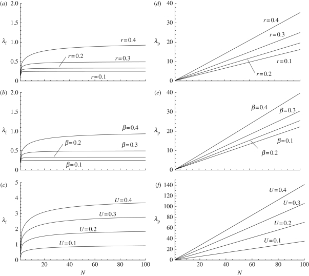
when the number of cultural traits, c, and the population size, N, are large (equations (A 8)–(A 13) of appendix A). This equation shows that λ_f tends to increase with increasing values of each parameter (U, β, r and N). The second term in equation (3.4) accounts for the effect of stochastic fluctuations in number of individuals carrying a focal trait (i.e. sampling effects). These stochastic effects are greater when there are fewer exemplar individuals in the population from whom to copy traits, which tends to decrease the number of traits carried by a focal individual. The exact expression for λ_f is graphed in figure 1, but numerical investigations suggest that λ_f is very well approximated by equation (3.4) for most parameter values.

Figure 1.

(a–c): mean number λ_f of cultural traits per individual graphed as a function of population size N for various parameter values. In (a), the innovation and the transmission rates are held constant (U = 0.1 and β = 0.5), while the recall rate, r, varies; from the top to the bottom curves, r = 0.4, 0.3, 0.2 and 0.1. In (b), the innovation and recall rates are held constant (U = 0.1 and r = 0.5), while the transmission rate β varies; from the top to the bottom curves β = 0.4, 0.3, 0.2 and 0.1. In (c), the transmission and memory rates are held constant (β = 0.1, and r = 0.5), while the innovation rate U varies; from the top to the bottom curves U = 0.4, 0.3, 0.2 and 0.1. (d–f): mean population number of cultural traits λ_p graphed as a function of population size N for exactly the same combinations of parameter values as given in (a–c).

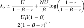
The expected number λ_p of different cultural traits in the population when it becomes large is approximated by

3.5

which increases with NU, the product of population size and the innovation rate per individual (equations (A 8)–(A 14)). When r = 0 and the third term is neglected, this equation reduces to a result established previously by Strimling et al. [24]. Hence, when individuals carry an infinite number of cultural traits (c → ∞), update their traits through social learning by random copying (e.g. according to equation (3.3)), and have no memory (r = 0), our model becomes similar to that of Strimling et al. [24]; see also equation (A 11) of appendix A. Note, however, that the model of Strimling et al. [24] is based on different biological assumptions than our model. An ‘updating’ event of cultural traits in their case actually involves a single individual dying and its replacement individual inventing new traits at rate U and adopting each trait of a randomly sampled cultural parent with probability β, which suggests that models with long-living forgetful individuals can be recast as models with short-living individuals with perfect memory. The exact expression for λ_p is graphed in figure 1, but as was the case for the individual mean, numerical investigations suggest that λ_p is generally well approximated by equation (3.5) even for population sizes as small as N = 10.

Figure 1 suggests that the average number of different traits carried by an individual can be low while at the same time the average number of different traits in the population may be very high, which suggests that the proportion of shared traits between two individuals, φ, is likely to be low. When the population size becomes large, this proportion is approximated by

3.6

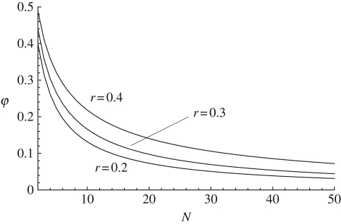
We see first that as population size increases, φ decreases and approaches zero and, second, that φ does not depend on the innovation rate U (equations (A 8)–(A 15)). Hence, it is mainly social learning that causes the homogenization of the population, and the higher the memory the higher the proportion of shared traits because individuals tend to remember invented traits, which can then be copied by others. The exact expression for φ is graphed in figure 2, and the approximation of φ given by equation (3.6) is good even for small population size when the parameters β and r are small; otherwise the approximation requires that population size is large (N > 50).

Figure 2.

Probability φ that two individuals carry at least one cultural trait in common for U = 0.1 and β = 0.5, while the recall rate, r, varies; from the top to the bottom curves, r = 0.4, 0.3 and 0.2.

While there might be high cultural diversity in the population at steady-state under the random copying social learning rule, two individuals are unlikely to share the same cultural traits when the population size becomes large (figures 1 and 2). In order to investigate the extent to which this depends on the assumptions of the learning rule (equation (3.3)), we now analyse the values that λ_f, λ_p and φ can take under other social learning rules.

(c). Beyond random copying: sensitivity to minority and biased conformist transmission

In copying the cultural traits of others in the population, individuals may express various preferences resulting in different social learning rules [22]. Here, we consider preferences that result in sensitivity to minority or biased conformist transmission. These two cases can be analysed with the following social learning rule:

3.7

When α = 1 we recover the random copying social learning rule (equation (3.3)), while for α < 1 the probability of adopting a focal cultural trait is increased at low prevalence of the trait in the population (e.g. sensitivity to minority). When α > 1 we have biased conformist transmission, and the social learning rule curves down at low prevalence (i.e. it is convex) and up at high prevalence.

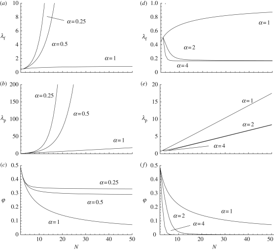
How λ_f, λ_p and φ vary as functions of the parameters for these two social learning rules is graphed in figure 3. Sensitivity to minority (α < 1) increases both λ_f and λ_p relative to the random copying rule. Each individual is then likely to carry more traits. But for a given value of population size N, the difference between the mean number of traits carried by an individual (λ_f) and the mean number of traits expressed by all individuals in the population (λ_p) decreases. Hence, the population becomes more homogeneous in the expression of cultural traits. This can also be noted from figure 3, which shows that the proportion of shared traits between two individuals, φ, no longer goes to zero as population size increases (as occurred under random copying, figure 2) but reaches a steady-state value. This is because under sensitivity to minority if there is one individual carrying a focal trait, then it is very likely to be copied by another individual in the population, thereby increasing the proportion of shared traits.

Figure 3.

(a–c): λ_f, λ_p and φ graphed as functions of population size N for the ‘sensitivity to minority’ social learning rule (equation (3.7) with α < 1) with U = 0.1, β = 0.5 and r = 0.4. From the top to the bottom curves α = 0.25, 0.5 and 1. (d–f): λ_f, λ_p and φ graphed as functions of population size N for the conformist transmission social learning rule (equation (3.7) with α > 1) with U = 0.1, β = 0.5 and r = 0.4. From the top to the bottom curves α = 1, 2 and 4 (in d and e the lines for α = 2 and α = 4 are nearly indistinguishable).

Exactly opposite patterns to those of sensitivity to minority are observed under conformist transmission (equation (3.7) with α > 1), where both λ_f and λ_p decrease relative to the random copying rule and at the same time the population becomes more heterogeneous (figure 3). Hence, as α increases, the proportion of shared traits between two individual traits decreases rapidly as population size increases (compare figure 3c and 3f). This is because in the limit of a large number of traits, the frequency of appearances of each trait will be low (as innovation per trait is very low). Under conformist transmission individuals are unlikely to copy a trait that is at low frequency in the population (say a trait carried by a single individual); hence conformist transmission will inhibit the increase in the number of individuals carrying a focal trait, thus decreasing the proportion of shared traits in the population.

(d). Culturally structured population

So far we have assumed that individuals interact at random in the population, but in reality interactions may be localized as individuals copy cultural traits from neighbours rather than from strangers [25]. In order to take such cultural viscosity into account, we now assume that the population consists of an infinite number of groups, each of finite size N. When a focal individual in a given focal group updates a focal trait, we assume that it copies a random individual from its group with probability (1 − m) and copies another individual, randomly sampled from another group, with probability m, where the parameter m can be thought of as the probability of learning from outsiders. With these assumptions, the social learning rule is now given by

3.8

where y is the frequency of individuals in the focal group (excluding the focal individual) that carry the focal trait and ρ_f = ∑_i x(i)i/N is, as before, the probability that an individual randomly sampled from the total population carries a focal trait. Here x(i) is the stationary probability that a group in the population contains i individuals that carry the focal trait, in which case the focal individual copies one of these with probability i/N (see also appendix Ab).

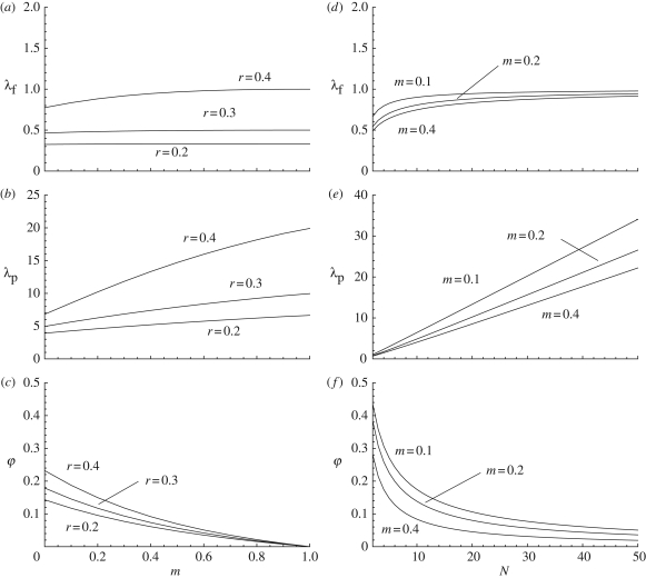
How λ_f, λ_p and φ vary as functions of the probability m of learning from outsiders (‘cultural migration’) in the presence of random copying (equation (3.3)) is illustrated in figure 4. As the rate m of cultural migration increases, the number of cultural traits expressed by a single individual or by all members in a group increases. This is because, as cultural migration increases, individuals tend to copy traits from others in the population with a fixed probability (i.e. second term in equation (3.8)), instead of copying individuals locally where the prevalence of a focal trait may fluctuate as a result of sampling effects. When m = 0, the model becomes similar to the panmictic finite population size model investigated above (equation (3.3) in equation (A 1)), which can be interpreted as the situation where a focal group of size N is completely isolated from other groups in the population (no exchange of cultural traits between groups). By contrast, when m = 1, the model becomes similar to the situation of a panmictic population of infinite size (equations (A 16)–(A 20) of appendix A), in which case there are no longer fluctuations in abundance frequencies owing to finite population size.

Figure 4.

(a–c) λ_f, λ_p and φ graphed as functions of the migration rate m for N = 20, U = 0.1 and β = 0.5 for the random copying social learning rule with migration (equation (3.8)). From the top to the bottom curves in each graph r = 0.4, 0.3 and 0.2. (d–f): λ_f, λ_p and φ graphed as functions of group size N for U = 0.1, β = 0.5 and r = 0.4. From the top to the bottom curves m = 0.1, 0.2 and 0.4.

It follows from these considerations that the proportion of shared traits between individuals decreases as the rate of ‘cultural migration’ m increases (figure 4), and, as was the case for the panmictic model, the proportion of traits shared between individuals decreases as population size increases, which also reduces the magnitude of the sampling effects. The effect of demographic factors (here N and m) on the level of cultural homogeneity φ within groups is, therefore, qualitatively similar to the effect of these factors on the probability that two individuals carry identical variants in standard neutral evolutionary models, whether the variants are genetic [1,26] or cultural [5].

(e). Norms

So far we have assumed that the cultural traits are expressed as a result of decisions taken by individuals alone. But some decisions are taken collectively; they are made not by individuals acting alone, but by groups of individuals. Suppose that the group of N individuals has to choose whether or not to adopt a cultural trait at the population level, which we call a norm. Thus a norm is interpreted as being a cultural trait that results from the aggregation of cultural traits expressed by single individuals. In reality, the aggregation process may be a function of the cultural profiles of all individuals in the population and is therefore likely to be a complicated function of the expression of several different traits by each individual.

For simplicity, suppose that a norm results from the aggregation of the expression pattern of a focal trait only. We can then define the aggregation function A(o₁,o₂, … , o_N) ∈ {0,1}, which maps the cultural pattern of the focal trait into presence or absence of the norm, where o_j is the cultural state at the focal position of the jth individual. In order to evaluate the likelihood that the norm is expressed for various transmission rules, we introduce an ε-majority rule A_ε such that A_ε = 1 if the number of individuals carrying the trait at the focal position in the population is equal to or greater than ε: that is, A_ε = 1 if ∑_{i =1}^N, o_i ≥ ε; A_ε = 0 otherwise. Given an ε-majority rule, the probability η_ε that a norm is chosen by the individuals in the population is

3.9

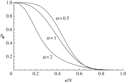
from which we can evaluate the probability of occurrence of a norm for the ε-majority rule under the sensitivity to minority and biased conformist social learning rules (the choice of the ε-majority rule and the implementation of the norm itself are other problems, whose analysis would entail modelling the games individuals are playing in the population). This is graphed in figure 5. The probability of adopting the norm is greater under sensitivity to minority than under biased conformist transmission unless the threshold ε becomes very high. This is due to the fact, already encountered, that at low prevalence the sensitivity to minority social learning rule tends to increase the prevalence of a trait in the population because individuals not carrying that trait tend to adopt it.

Figure 5.

Probability η_ε (equation (3.9)) of occurrence of an ε-majority rule for various social learning rules (equation (3.7)) as a function of the threshold frequency ε/N of individuals carrying the trait below which the norm is not chosen by the individuals in the population. The top curve is for sensitivity to minority with α = 0.5, the curve in the middle is for random copying (α = 1), and the bottom curve is for conformist transmission with α = 2. The other parameter values for all curves are U = 0.1, β = 0.5, r = 0.4 and N = 20.

4. Discussion

We have presented a model for the accumulation of independent cultural traits through individual and social learning in finite populations. This multi-trait cultural model allows us to characterize the cultural diversity at the individual and population levels at the steady state of the learning dynamics and as a function of various features of the demography and the rules of cultural transmission. Our model has features in common with multilocus population genetic models [16], and is directly related to previous models of stochastic cultural evolution. When individuals in the population carry only a single trait (c = 1), it is similar in essence to the model by Lumsden & Wilson [22]. In contrast, when individuals may carry an infinite number of cultural traits (c → ∞), social learning occurs through random copying (equation (3.3)), and individuals have no memory (r = 0), our model becomes similar to the multi-trait model of Strimling et al. [24].

Our results suggest that when individuals may invent infinitely many cultural traits, the stationary individual and population-wide distributions of the number of distinct traits are Poisson. The means of these two trait-number distributions (λ_f and λ_p) then fully characterize the cultural diversity at the individual and population levels because of our assumption of the independence of the cultural traits, which is probably the most stringent of our model. But this assumption allows us to establish a null model for the trait number distribution that is tractable and to which other results can be compared. For instance, the Poisson distribution plays a central role in population genetics as the null model of reproduction (e.g. the ideal Wright–Fisher population, [3,16,27]), and it is by reference to this model that the effects of relaxing demographic assumptions may be assessed. One could thus relax the assumption of the independence of traits, and investigate how this might affect the steady-state distribution of trait-number at both the individual and population levels. Further, memory (r) might be modelled as a decreasing function of the number of traits an individual carries, or the total innovation rate (U) might be modelled as an increasing function of this number.

The means of the trait-number distributions (λ_f and λ_p) and the proportion of traits shared between two randomly sampled individuals (φ) are critically affected by the demographic details and the social learning rules. In a panmictic population with random copying (equation (3.3)), there might be high cultural diversity in the population, while at the same time single individuals may carry only a few traits (figure 1). The population will then be culturally heterogeneous, as any two individuals are unlikely to share cultural traits in common (figure 2). While this pattern seems somewhat counterintuitive as we expect individuals within populations to share cultural traits, random copying is probably the social learning rule that makes the accumulation model presented here closest to standard neutral models of population genetics. Indeed, it was shown by Strimling et al. [24] that with a change of variable one can recover from the mean number of traits λ_p, the expected number of different variants segregating in a population in a one-trait model, a well-known result in population genetics [10,16].

When social learning does not occur by random copying, very different levels of cultural homogeneity are observed. With biased conformist transmission two randomly chosen individuals are very unlikely to share common cultural traits, even when population size is low (figure 3). In contrast, when individuals express sensitivity to a minority, single individuals carry more cultural traits, two randomly chosen individuals are very likely to share common cultural traits, and cultural homogeneity of the population is increased (figure 3). These opposite patterns follow from the fact that if there is only one individual carrying a focal trait, then it is very likely to be copied by another individual under sensitivity to minority. By contrast, that trait is very unlikely to be copied by another individual under biased conformist transmission, thus preventing an increase in number of the focal traits in the population. Although this inhibiting effect of biased conformist transmission for the accumulation of cultural traits has not been recognized in the literature, one expects it to be observed more generally as most traits are likely to appear initially as a single (or a few) copy(ies) in a population.

Introducing population subdivison by allowing individuals to learn from others outside a focal group reduces the local fluctuations in abundance frequencies owing to sampling effects in finite populations. The result is an increase in the number of different traits carried by individuals (figure 4). This, in turn, decreases the level of shared traits within groups, φ, which also decreases with group size in exactly the same way as in a panmictic population (compare figures 2 and 4). The effects of the two demographic factors, m and N, are qualitatively similar to the effect of spatial structure on the distribution of genotypes within and between groups (e.g. [1–3]). Hence, the effects of demographic factors on the trait-number distribution appear to be qualitatively equivalent to their effects on the distribution of variants of a single gene (e.g. [1–3]).

We have assumed that infinitely many cultural traits may be invented but the number of possible independent cultural traits may be finite. From a qualitative point of view, allowing for a finite number of traits should not affect the main results reported here, because the assumption that all c traits are independent of each other allowed us to derive our results from single-trait dynamics; the number of different traits carried by an individual (or by all individuals in the population) then varies directly with c, holding everything else constant.

We have not incorporated organismal birth and death into our model. Including such features should not affect the qualitative results reported here if the number of updating events occurring during the lifespan of an individual is sufficiently large that the updating process converges approximately to stationarity. It would be interesting, however, to study the accumulation of cultural traits in the presence of a few transmission rounds within the lifespan of an individual and with intergenerational effects, which would follow from including organismal birth and death.

Overall, our results suggest that the cultural diversity at both the individual and population levels (λ_f and λ_p) are increasing functions of the demographic factors, namely the population size (N) and the cultural migration rate (m), and of the organismal parameters, namely the number of cultural traits (c) an individual may possibly carry, the per trait innovation rate (μ), the memory (r), and the probability of adopting traits learned socially from others (β). Hence, in addition to the demographic parameters and the innovation rate, which are well known to play an important role in describing diversity in classical population genetic models, the memory, and the intensity of cultural transmission (as well as the mode of transmission) are also likely to affect patterns of cultural diversity at both the individual and the population levels. All of the organismal features encountered may be under partial genetic control and thus subject to genetic evolutionary change. We can speculate that such genetic control of these parameters may have implications for the evolution of modern humans from their less culturally capable predecessors, or for their success in overcoming less cultural contemporary groups.

Appendix A

(a). Stationary abundance distribution

(i). Asynchronous updating

In this appendix, we present an explicit expression for the stationary probability x(i) that i individuals in the population carry a focal trait under asynchronous updating. For this case, the updating process follows a so-called birth–death process (e.g. [16, p. 91], [17, p. 269], [23]), and the stationary distribution is given by

A 1

where x(0) is chosen so that ∑_i=0^Nx(i) = 1; b(h) is the probability that, conditional on an updating event taking place in a population with h individuals carrying a focal cultural trait, a new individual carries that trait after updating; and d(h) is the probability that, conditional on an updating event taking place in a population with h individuals carrying the cultural trait, one fewer individual carries the trait after updating ([16, eqn 2.162]).

The values of b(h) and d(h) can be obtained from equations (3.1)–(3.2) by noting that in a population with h individuals carrying the focal trait, an individual not carrying it is sampled to update its cultural loci with probability (N − h)/N, in which case it carries the focal trait after updating with probability q(h), while an individual carrying the focal trait is sampled to update its cultural loci with probability h/N, in which case it does not carry the trait after updating with probability 1 − p(h). Thus

A 2

and

A 3

and on insertion of equations (3.1)–(3.2), one has

A 4

and

A 5

Note that these equations imply that a single individual updates all its cultural traits simultaneously. Alternatively, one could assume that a single individual in the population updates one cultural trait per unit time, in which case the right-hand sides of equations (A 4)–(A 5) would be divided by c, which will not affect the stationary abundance distribution but only the rate of convergence to equilibrium.

(ii). Linear updating

Substituting equation (3.3) and equations (A 4)–(A 5) into equations (A 1), we find after rearrangement that the stationary distribution can be expressed as

A 6

which allows us to evaluate ρ_f and ρ_p by using equations (2.4)–(2.5). The resulting expressions are complicated and involve hypergeometric functions, but can be easily calculated numerically, for example with Mathematica [28]. In the absence of memory, i.e. r = 0, however, it can be shown that

A 7

which is the same probability as that found in a population of infinite size (see equation (A 20)). No such simple expression was found for ρ_p when r = 0. In order to obtain more tractable analytical expressions than equation (A 6), we will evaluate the trait-number distributions in the limit as the number of cultural traits and population size become large.

(b). Culturally structured population

In a culturally structured population with an infinite number of groups following the same updating process, groups affect each other in a deterministic way [29]. Then, x(i) gives both the probability that i individuals in a focal group carry a focal trait (and thus satisfies equation (A 6)) and the probability that a randomly sampled group in the population consists of i individuals carrying a focal trait, which may affect the transition probabilities of the state of a focal group. This is the case for the updating probabilities p(h) and q(h) given by equations (3.1)–(3.2) (with equation (3.8)) of the main text, which are now functions of the stationary distribution itself through their dependence on ρ_f. Thus we can no longer obtain an explicit expression for x(i), which is now implicitly determined (e.g. insert equation (3.8) into equations (3.1)–(3.2), then equations (3.1) and (3.2) into equations (A 4)–(A 5)). This distribution can, however, be evaluated numerically from ρ_f = ∑_ix(i)i/N, which has a closed form once equations (3.1)–(3.2), equation (3.8) and equations (A 4)–(A 5) have been inserted into equation (A 1). From this, we can then compute λ_f, λ_p and φ, which are presented in figure 4.

(c). Large population size

(i). Large population size approximation

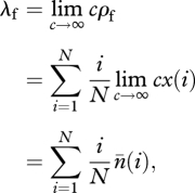
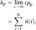
Our aim in this section is to obtain a large population size approximation for λ_f, λ_p and φ when the stationary abundance distribution is given by equation (A 6). To that end, we use the variable , which can be interpreted as the expected number of traits of popularity i in the population (a quantity introduced by [24]) in the limit of an infinitely large number of traits. With this, we have

A 8

A 9

and

A 10

where we used equations (2.4)–(2.6).

By using μ = U/c in equation (A 6), it can then be shown that the expected number of traits of popularity i in the limit of an infinitely large number of traits (c → ∞) is given by

A 11

which, when r = 0, is equation (2) of Strimling et al. [24]. The derivation of equation (A 11) from equation (A 6) by using and μ = U/c is a bit messy to check by hand but it can easily be done with a symbolic algebra system such as Mathematica [28].

A first order Taylor expansion of equation (A 11) near N = ∞ with Mathematica gives, for N > 2 and 0 < β < (N − 1)/N,

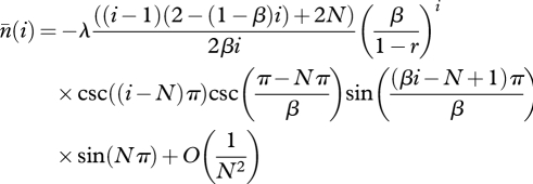A 12

where csc(·) is the cosecant function. Substituting equation (A 12) without the O(1/N²) term into equations (A 8)–(A 10) and letting N → ∞ in the summation gives

A 13

A 14

and

A 15

Substituting equations (A 13) and (A 15) into equation (2.7) gives φ ≃ β /[N(1 − β − r)] + O(1/N²). Note that N ≃ N − 1 when N is large and that Strimling et al. [24] used a different approximation in order to derive their expression for λ_p (their proposition 1).

(ii). Infinite population size

In this section, we present an equation for the dynamics of ρ_f for a focal trait when the population size becomes infinitely large. In that case, we can neglect fluctuations in the number of individuals carrying the trait during updating because the probability that a randomly sampled individual carries the trait converges to its expectation. Then, the probability p(ρ_f) that a focal individual who carries the focal trait before updating also carries that trait after updating can be written as a function of the expectation ρ_f that a randomly sampled individual from the population carries the trait. Similarly, the probability q(ρ_f) that a focal individual who does not carry the focal trait before updating carries it after updating becomes a function of ρ_f. Hence, the probability ρ′_f that a focal individual carries the trait at the focal locus just after it has updated that position can be expressed as

A 16

and given the forms of p(·) and q(·), equation (A 16) can be solved for ρ_f at equilibrium; that is when ρ′_f = ρ_f.

For our model, with random copying, the transition probabilities are, from equations (3.1)–(3.2), given by

A 17

and

A 18

Substituting equations (A 17)–(A 18) into equation (A 16) and solving for ρ_f, the equilibrium probability that an individual carries the focal trait becomes

A 19

and in the absence of memory, r = 0, this reduces to

A 20

Substituting μ = U/c into equation (A 19) and taking λ_f = lim_c→∞ cρ_f, we find that the mean of the trait-number distribution is given by λ_f = U/(1 − β− r).

References

- 1.Wright S. 1931. Evolution in Mendelian populations. Genetics 16, 97–159 [DOI] [PMC free article] [PubMed] [Google Scholar]
- 2.Gillespie J. H. 2004. Population genetics: a concise guide. Baltimore, MD: Johns Hopkins University Press [Google Scholar]
- 3.Hartl D., Clark A. G. 2007. Principles of population genetics, 4th edn Sunderland, MA: Sinauer [Google Scholar]
- 4.Cavalli-Sforza L., Feldman M. W. 1973. Models for cultural inheritance 1. Group mean and within group variation. Theoret. Popul. Biol. 4, 42–55 (doi:10.1016/0040-5809(73)90005-1) [DOI] [PubMed] [Google Scholar]
- 5.Cavalli-Sforza L., Feldman M. W. 1981. Cultural transmission and evolution. Princeton, NJ: Princeton University Press [Google Scholar]
- 6.Boyd R., Richerson P. J. 1985. Culture and the evolutionary process. Chicago, IL: University of Chicago Press [Google Scholar]
- 7.Lynch M., Gabriel W. 1990. Mutation load and the survival of small populations. Evolution 44, 1725–1737 (doi:10.2307/2409502) [DOI] [PubMed] [Google Scholar]
- 8.Lynch M., Bürger R., Butcher D., Gabriel W. 1993. The mutational meltdown in asexual populations. J. Heredity 84, 339–344 [DOI] [PubMed] [Google Scholar]
- 9.Kimura M., Crow J. F. 1964. The number of alleles that can be maintained in a finite population. Genetics 49, 725–738 [DOI] [PMC free article] [PubMed] [Google Scholar]
- 10.Ewens W. J. 1972. The sampling theory of selectively neutral alleles. Theoret. Popul. Biol. 3, 87–112 (doi:10.1016/0040-5809(72)90035-4) [DOI] [PubMed] [Google Scholar]
- 11.Hubbell S. P. 2001. The unified neutral theory of biodiversity and biogeography. Princeton, NJ: Princeton University Press [Google Scholar]
- 12.Bentley R. A., Hahn M. W., Shennan S. J. 2004. Random drift and culture change. Proc. R. Soc. Lond. B 271, 1443–1450 (doi:10.1098/rspb.2004.2746) [DOI] [PMC free article] [PubMed] [Google Scholar]
- 13.Lumsden C. J., Wilson E. O. 1981. Genes, mind and culture. Harvard, MA: Harvard University Press [Google Scholar]
- 14.Enquist M., Ghirlanda S., Jarrick A., Wachtmeister C. A. 2008. Why does human culture increase exponentially? Theoret. Popul. Biol. 74, 46–55 (doi:10.1016/j.tpb.2008.04.007) [DOI] [PubMed] [Google Scholar]
- 15.Lehmann L., Feldman M. W. 2009. Coevolution of adaptive technology, maladaptive culture, and population size in a producer–scrounger game. Proc. R. Soc. B 276, 3853–3862 (doi:10.1098/rspb.2009.0724) [DOI] [PMC free article] [PubMed] [Google Scholar]
- 16.Ewens W. J. 2004. Mathematical population genetics. New York, NY: Springer [Google Scholar]
- 17.Grimmett G., Stirzaker D. 2001. Probability and random processes. Oxford, UK: Oxford University Press [Google Scholar]
- 18.Wright S. 1951. The genetical structure of populations. Ann. Eugenics 15, 323–354 [DOI] [PubMed] [Google Scholar]
- 19.Crow J. F., Aoki K. 1984. Group selection for a polygenic behavioral trait: estimating the degree of population subdivision. Proc. Natl Acad. Sci. USA 81, 6073–6077 (doi:10.1073/pnas.81.19.6073) [DOI] [PMC free article] [PubMed] [Google Scholar]
- 20.Cockerham C. C., Weir B. S. 1987. Correlations, descent measures: drift with migration and mutation. Proc. Natl Acad. Sci. USA 84, 8512–8514 (doi:10.1073/pnas.84.23.8512) [DOI] [PMC free article] [PubMed] [Google Scholar]
- 21.Slatkin M. 1991. Inbreeding coefficients and coalescence times. Genet. Res. 58, 167–175 (doi:10.1017/S0016672300029827) [DOI] [PubMed] [Google Scholar]
- 22.Lumsden C. J., Wilson E. O. 1980. Translation of epigenetic rules of individual behavior into ethnographic patterns. Proc. Natl Acad. Sci. USA 77, 4382–4386 (doi:10.1073/pnas.77.7.4382) [DOI] [PMC free article] [PubMed] [Google Scholar]
- 23.Karlin S., Taylor H. M. 1975. A first course in stochastic processes. San Diego, CA: Academic Press [Google Scholar]
- 24.Strimling P., Sjöstrand J., Enquist M., Eriksson K. 2009. Accumulation of independent cultural traits. Theoret. Popul. Biol. 76, 77–83 (doi:10.1016/j.tpb.2009.04.006) [DOI] [PubMed] [Google Scholar]
- 25.Feldman M. W., Cavalli-Sforza L. L. 1976. Cultural and biological evolutionary processes, selection for a trait under complex transmission. Theoret. Popul. Biol. 9 238–259 (doi:10.1016/0040-5809(76)90047-2) [DOI] [PubMed] [Google Scholar]
- 26.Rousset F. 2004. Genetic structure and selection in subdivided populations. Princeton, NJ: Princeton University Press [Google Scholar]
- 27.Karlin S., McGregor J. 1968. The role of the Poisson progeny distribution in population genetic models. Math. Biosci. 2, 11–17 (doi:10.1016/0025-5564(68)90003-5) [Google Scholar]
- 28.Wolfram S. 2003. Mathematica, 5th edn Cambridge, UK: Cambridge University Press [Google Scholar]
- 29.Chesson P. L. 1981. Models for spatially distributed populations: the effect of within-patch variability. Theoret. Popul. Biol. 19, 288–325 (doi:10.1016/0040-5809(81)90023-X) [Google Scholar]