Geographic boundary analysis in spatial and spatio-temporal epidemiology: Perspective and prospects

Abstract

Geographic boundary analysis is a relatively new approach that is just beginning to be applied in spatial and spatio-temporal epidemiology to quantify spatial variation in health outcomes, predictors and correlates; generate and test epidemiologic hypotheses; to evaluate health-environment relationships; and to guide sampling design. Geographic boundaries are zones of rapid change in the value of a spatially distributed variable, and mathematically may be defined as those locations with a large second derivative of the spatial response surface. Here we introduce a pattern analysis framework based on Value, Change and Association questions, and boundary analysis is shown to fit logically into Change and Association paradigms. This article addresses fundamental questions regarding what boundary analysis can tell us in public health and epidemiology. It explains why boundaries are of interest, illustrates analysis approaches and limitations, and concludes with prospects and future research directions.

1. Introduction

“A boundary is that which is an extremity of anything”

Euclid’s Elements: Book 1

Why employ boundary analysis? Three reasons are paramount. First, boundaries are where the values of a variable are changing rapidly, and are often of direct scientific interest since they are zones of dynamic geographic change (e.g. edges of neighborhoods defined by socio-economic status, employment and deprivation; zones of population mixing in population genetics; the edges of disease clusters in public health; places where environmental exposures are changing and so on). In spatial and spatio-temporal epidemiology boundary analysis may be used to identify edges of populations homogeneous in health outcomes, covariates and/or risk factors. This is useful when identifying study populations, targeting groups for health interventions, when siting health screening facilities, and for exploring relationships between environmental exposures and health outcomes (Jacquez and Greiling 2003).

Second, boundary analysis allows us to better define sample populations, increasing our ability to resolve underlying functional relationships. It is difficult to accurately assess odds ratios, fit models and assess health-environment relationships within homogeneous areas – both exposed and not-exposed groups are required in order to find an effect. A common mistake in geographic sampling design is to focus on those sub-populations with a high risk in the health outcome of interest. In these instances we shouldn’t be surprised by an inability to reveal underlying health-environment relationships, since the range of variability needed to resolve them is lacking. Consider for example Figure 1, left, which shows no relationship between the values of exposure and health outcome variables sampled from within an area homogeneous in the values of these variables – e.g. away from geographic boundaries in the health outcome. By placing samples across such boundaries the analyst is better able to capture the full range of variability in the variables, and to detect the functional relationship (Figure 1, right).

Figure 1.

Failure to sample a representative range of variability can lead one to miss health (H) environment (G) relationships. Sampling from within a geographic cluster (map not shown) will yield homogeneous values such as shown in the rectangle (left). Sampling across geographic boundaries (map not shown), which are zones of rapid change in values, results in a sample drawn from the full range of variability, as shown by the observations in circles (right). In practice one first identifies boundaries on the map of the variables and then samples across them (e.g. on both sides of and within the boundaries themselves). These graphs illustrate that zones of rapid change identified by geographic boundary analysis can be used to guide sample design.

Third, boundary analysis allows us to relax unrealistic and/or unfounded assumptions regarding the form of the functional relationships between measures of human health and its predictors. Tests for boundary overlap require that the variables whose association is being assessed covary only to the extent that change in one results in change in the other, and are less stringent about the form of the relationships between the variables. In practice boundary overlap may be assessed in several ways, including minimum average distance between health and environment boundaries (Jacquez 1995), area intersection operations (Maruca and Jacquez 2002), and the direct overlap of the boundaries themselves. None of these approaches make assumptions regarding the functional form of the underlying health environment-relationship. Contrast overlap analysis with approaches such as the Pearson product-moment correlation coefficient, which assumes a linear dependence between the variables. Boundary overlap does not make assumptions regarding the form of the model of dependence. This is a critical assumption to relax since relationships of biological interest are often non-linear and may not even be monotonic.

Boundary analysis informs spatial pattern analysis, which is classified for convenience into Value, Change, and Association questions. These 3 questions are similar to those identified as important to ask of an atlas map by epidemiologists (see Pickle 2009); these in turn are similar to Bertin’s classification of visualization tasks (Bertin 1974). Value questions have to do with the values of the variables surveyed, and how they are arranged in geographic space. Value questions are explored using disease mapping through spatial point distributions, choropleth maps (Richards, Berkowitz et al. 2010) and related techniques. This in many ways is the point of departure for spatial epidemiology, with examples such as Snow’s Cholera map (Snow 1855) and disease Atlases [see (Pickle 2009) for a review]. Value questions are the domain of disease clustering, which seeks to identify spatially contiguous areas of high or low disease occurrence. This includes techniques for case-control data (Cuzick and Edwards 1990), case count and population at risk data (Takahashi, Yokoyama et al. 2004; Tango and Takahashi 2005; Kulldorff, Song et al. 2006) and disease rates (Rushton, Peleg et al. 2004).

Change questions have to do with higher order properties of spatial response surfaces, such as gradients (how values change through geographic space). Boundary analysis is the dual of cluster analysis, in that the former seeks to identify geographic areas where the health outcome (e.g. disease risk) is changing rapidly (e.g. where the spatial response surface has large derivatives), while the latter seeks to identify local populations with high relative risks (e.g. where the derivative is near zero and disease risk is high). Methods for detecting boundaries date back at least to 1951 (Womble 1951), and include geostatistical (Goovaerts 2008), Bayesian (Lu and Carlin 2005), wavelet (Csillag, Boots et al. 2001), distribution-based (Jacquez, Kaufmann et al. 2008), difference (Monmonier 1973), as well as distribution-free approaches (Hall 2008). Several methodological reviews are available for readers who wish to become more familiar with these techniques (Fortin 1994; Jacquez, Maruca et al. 2000; Kent 2006).

Association questions seek to relate spatial pattern in one variable or set of variables to the pattern in another set of variables, and include diverse methods such as boundary overlap (Jacquez 1995), map area intersection (Sadahiro and Umemura 2001; Maruca and Jacquez 2002; Robertson, Nelson et al. 2007), spatial regression modeling (Mantel 1967; Greenland and Robins 1994; Dormann 2007; Fotheringham 2009), geostatistical analysis (Goovaerts 2009) and Bayesian disease mapping (Ma, Lawson et al. 2007; Lawson and Banerjee 2008). As noted above, tests for boundary overlap evaluate association by determining the extent to which features on spatial response surfaces coincide.

This paper is a perspective on some of the issues and problems in boundary analysis in public health. It begins with a description of technological and societal trends, alternative approaches to pattern recognition, and then focuses on statistical approaches that support probabilistic assessment of how unusual a pattern is under a specified null hypothesis. Value, Change, and Association questions are then described in detail. This perspective is illustrated with a motivating example: the pattern of leukemia incidence in 8 counties in New York State. This pattern is related to the location of sites contaminated with TriChloroethylene (TCE), using a step-wise approach involving Value, Change and Association questions. The importance of pattern recognition in extracting knowledge from the burgeoning information stream made possible by emerging technologies is described, as is the role of pattern analysis in scientific inquiry. The author concludes with a discussion of current needs such as improved null spatial models, and speculates on the future of the field.

2. Technological and Societal Trends

Recent advances in remote sensing are providing hyperspectral imagery at the sub-1 meter scale for most locations on earth, and on weekly and even daily sampling intervals (Gail 2007; Plaza, Benediktsson et al. 2009). The analysis of remotely sensed imagery such as LandSat is beginning to be used to assess environmental health risks in cancer (Maxwell, Meliker et al. 2010), and is an important tool in the quantification of models for vector-born and infectious diseases (Gorla 2007). The emerging field of proteomics is elucidating relationships between the human genome and the production of enzymes and proteins, and is ultimately expected to increase our understanding of individual-level response to all manner of environmental exposures, including nutrients, pathogens, and toxic compounds (Verma 2009). The emergence of ubiquitous computing and data acquisition through wireless devices, internet2, agent-based computing (e.g. bots), the sensorweb (Churcher and Foley 2009) and the miniaturization of sensors is making it possible to monitor our environment in real time, and to simultaneously distribute this information to almost any location on the earth for processing, visualization and decision-making (Lahra and Kooistra 2010). Societal and regulatory trends, while always uncertain, seem to be towards a democratization of information, and an emerging consensus regarding the public’s “right to know” about industrial and governmental activities that impact the environment and human health. This is leading to the online availability of data describing industrial discharges into both air and water, and to the increased availability of public health information (not withstanding countervailing needs to protect confidentiality). Finally, the miniaturization of mechanical devices (e.g. MEMS, nano-medicine) will soon make possible the automation of interventions in individuals, in human populations (e.g. through drug and vaccine administration), and in the environment (e.g. clean-up bots) (Vinogradov 2010).

Technological and societal trends seem to lead to a data-rich future comprised of high spatial and temporal resolution data, available on temporal scales ranging from near real-time to weeks and months. Pattern recognition plays an integrative role because of its ability to identify objects and relationships in the stream of geotemporally referenced data. Without automated pattern recognition, we will not be able to make sense of the data cascade from the expanding array of satellites, airborne imaging platforms, bots, and miniaturized sensors; and will not be aware of important environmental changes, let alone capable of timely and effective response. Boundary analysis methods and approaches can be automated and applied to screen larger data sets to identify changes of importance to human health and the environment through space and time.

3. Statistical Pattern Recognition

There are several approaches to pattern analysis, including visual inspection, symbolic dynamic filtering (SDF), Bayesian Filters and Artificial Neural Networks (Ripley 1996; Rao, Ray et al. 2009), among others. Inferential approaches are used frequently in spatial epidemiology as they support tests of hypotheses and the evaluation of spatial structure in health outcomes, covariates, and risk factors (Rogerson and Yamada 2004; Rushton, Peleg et al. 2004; Richardson and Guihenneuc-Jouyaux 2009). This paper is primarily concerned with boundary analysis as a tool in statistical pattern recognition.

Statistical pattern recognition proceeds by calculating a statistic (e.g. spatial cluster statistic, boundary metric, etc.) that quantifies a relevant aspect of spatial pattern (Hastie, Tibshirani et al. 2009). The value of this statistic is then compared to the distribution of that statistic’s value under a null spatial model. This provides a probabilistic assessment of how unlikely an observed spatial pattern is under the null hypothesis (Waller 2008).

Both analytical (e.g. based on distribution theory) and randomization approaches are used to generate null distributions of spatial pattern statistics. The analytical approach assumes the underlying variables are sampled from a known distribution; it determines the distribution of the test statistic under the null hypothesis using that assumption (Jacquez, Kaufmann et al. 2008). This often entails conditions such as complete spatial randomness, or CSR, that have been widely criticized as untenable (Waller 2008; Goovaerts 2009). Randomization uses resampling techniques to generate an empirical null distribution, and thus has the advantage of being “distribution-free”. This has a cost in that randomization conditions strongly on the data, and inference is restricted only to the data being examined (Manly 2007).

4. Kinds of questions

Pattern recognition contributes in several areas of the scientific and analytic process. It plays an important role in data summarization and description by identifying salient features and structures in the data. It is used in hypothesis generation to stimulate explanatory conjectures regarding the origin of patterns. It is used in modeling (e.g. location-allocation models) to determine where facilities should be located, and in experimental design to specify optimal sampling strategies (e.g. to better capture spatial variance). Pattern recognition underlies some portion of cognitive theory regarding spatial thought, and can be a fundamental step in the development of scientific theory as well (for example, the theory of evolution emerged from Darwin’s recognition of spatial phenotypic variation). The author recognizes three kinds of pattern recognition questions -- Value, Change, and the search for Association.

5. Value questions

Consider some value questions often encountered in disease clustering and environmental analysis. Disease clustering is principally concerned with value questions such as “is there an excess of disease?”, and “where are disease rates significantly high?” In disease clustering several variants on pattern analysis emerge. Temporal clustering searches for excesses of disease in time series data. Spatial clustering searches for spatial clusters of disease. Space-time clustering seeks to identify clusters that occur in both space and time. These approaches usually are retrospective, working with existing data, although new surveillance techniques are being developed to determine when to “sound the alarm” as an excess of disease occurs in a stream of space-time data. Spatial scale is an important consideration in pattern recognition, and the disease clustering field recognizes general, local, and focused tests (Waller 2008). General tests search for clusters anywhere in the study area. Local tests identify where excesses occur within the study area. Focused tests seek to determine whether there is an excess of disease near putative sources, called “foci”.

Within this framework value questions include “Is there a hotspot? (global clustering)”, and “Where is the hotspot? (local clustering)”. Questions such as “Do case clusters occur around the injection well? (focused clustering)” have to do with matching spatial patterns and are association questions.

Value questions in environmental analysis include “where are heavy metals the highest?”, and “where does the toxin exceed EPA-approved maxima?” When quantifying variation in natural environments, ecologists may seek to identify patches defined by certain characteristics, such as biomass and available cover. These are all examples of Value questions.

6. Change questions

Change questions are concerned with where and how the values of a variable change through space and/or time. Several commonly used spatial techniques are founded on assumptions (e.g. stationarity, isotropy etc.) that correspond to a static worldview. The real world, however, is dynamic, and it makes sense to exploit this dynamic nature by investigating locations where variables change rapidly. Such “locations of rapid change” are known by different names depending on the field of study and method chosen. These include “edge”, “boundary”, “ecotone”, “transition zone”, “discontinuity”, and “margin”, among others. Change techniques examine zones of rapid change, the edges of phenomena, and the shape of spatial and space-time response surfaces. Consider some example questions.

In environmental fields, biotic response to change is known to be an important factor influencing habitat selection at the individual level and community structure at the ecosystem level (St-Louis 2004; Hall 2008). Hence, questions such as, “how fragmented is the environment?”, “what is the shape of the boundary?” and “where is the ecotone?” have direct ecological implications for imputing biotic relationships and for quantifying ecosystem dynamics (Kent 2006).

As the field of disease clustering has evolved the need to estimate the underlying risk function has become pressing. Corresponding Change questions include “where is the margin of the at risk population? ”, “what is the shape of the risk function? ”, “Where do disease rates change rapidly? ”, “Are there patches of disease outcomes?”, “How are the patches arranged? (e.g. homogeneous areas & global boundaries)” and “What is the shape of the disease cluster?”

7. Association questions

Association questions ask whether two or more geotemporally-referenced variables covary. Conventional approaches such as correlation and regression may be adjusted to accommodate spatial and temporal dependencies (Clifford, Richardson et al. 1989; Dutilleul 1993) but are not pattern-matching techniques. Within the framework of pattern recognition, association questions ask “are the space-time patterns in two or more variables similar?” This may be accomplished by determining, for example, whether areas of high values overlap significantly for 2 or more variables. It may also be addressed by determining whether boundaries overlap, whether the shape of the spatial response surfaces are similar, and whether objects defined on these response surfaces (e.g. hills, valleys, saddles) tend to coincide or repel. While conventional correlation/regression approaches and their analogs such as ANOVA are familiar, they do impose models of dependence that may or may not be appropriate in a given situation. Pattern-matching approaches are less stringent about the form of the relationships between the variables. They require that the variables whose association is being assessed covary only to the extent that change in one results in change in the other. Hence, assumptions regarding the form of the model of dependence aren’t necessary. This is a critical assumption to relax since relationships of biological interest are often non-linear and frequently are not even monotonic. Consider some examples illustrative of the ubiquity of non-linear relationships.

Toxicity curves

Toxicity curves, such as LD50, describe the time required for 1/2 of a population to die at a series of different doses of a toxic compound. As the dosage increases the number of days required to death decreases, and the relationship is usually monotonic decreasing. It is often nonlinear because the shape of the curve is determined at least in part by the metabolic capacity of the individual organisms. Most of the population can tolerate low doses and few die. As the dose increases metabolic capacity is overwhelmed and the time to achieve 50% die off decreases dramatically with only small increases in dose.

Essential nutrients

Many nutrients, such as selenium, are essential components of metabolic pathways and organisms do poorly and/or die when they are entirely absent. The organism does very well when the nutrient is present in trace amounts, but quickly becomes ill and dies when it is ingested at high doses.

Population growth curves

Well-known (if somewhat prosaic) notions such as an environment’s carrying capacity are based on the logistic curve that plots population size through time. Given a resource that is renewed at a constant rate, the population grows exponentially at first until the resource begins to limit growth, and plateaus at the carrying capacity

Epidemic curves

Epidemic curves plot the number of individuals in disease states such as susceptible, infected and immune, through time. Even for simple deterministic systems these plots are almost always non-linear, changing dramatically when the epidemic takes off, and reach a plateau once the endemic phase is achieved.

Space-time lags

Testing for association between a putative risk factor and subsequent disease is much more complicated when an appropriate time lag between exposure and disease must be determined. A major analytic problem is estimating an appropriate temporal lag. Rothman (Rothman 1981) defined the empirical induction period to be comprised of an induction period, within which critical exposures may occur, and a latency period between onset of disease (e.g. cancer) and diagnosis. Notice the induction period may be brief (e.g. as for infection transmission events) or on the order of years and decades (e.g. cancer, where accumulating genetic mutations mediated by environmental exposures and underlying mutation rates may be offset by DNA repair mechanisms). When information sufficient to specify a process-based model based on the mechanisms underlying disease progression is available, the temporal lag process may be estimated as the residency times in compartmental models, and has been shown to often follow an Erlang distribution (Jacquez 2002).

Non-linearity is thus the norm rather than the exception, and we frequently do not know even the form of the functional relationship, especially when working with observations on spatial systems that are subject to lags and discontinuities, and which violate assumptions of ergodicity, stationarity, and isotropy. How can one evaluate association questions when the form of the association is unknown, and when variables covary only over certain value ranges, or only at certain locations?

The answer is to evaluate association using pattern matching. Within the context of pattern recognition, association questions ask whether patterns quantified on two or more variables “match” -- by occurring nearby, and/or by having similar shapes. Example association questions include “Are the clusters of cases associated with the locations of hazardous waste sites?”, and “Is spatial pattern in health outcomes associated with:

• The environment? (exposure, behavior, neighborhood context, etc.),

• Population? (demography, marriage, birth, ethnicity etc.) and

• Genetics? ”

8. Example: Childhood leukemia in New York State

To motivate this framework consider an example describing leukemia incidence for 1978-1982 for 8 counties (Cayuga, Onondoga, Madison, Tompkins, Cortland, Chenango, Tioga, Broome) in upstate New York. Leukemia is a rare disease, and 592 cases occurred in a population of 1,057,673 in 790 census tracts or blocks (Figure 2). Waller (Waller, Turnbull et al. 1992) found a significant relationship between leukemia incidence and distance to a Monarch Chemical site that contaminated the groundwater with TCE. The population sizes are based on the 1980 U.S. census, and the data are publicly available (Waller 1994). The data analyzed are the incident case counts, populations at risk, and the incident number of cases per 1,000 population (the rate). We use the term “risk” to refer to an underlying, but unobservable leukemia risk. We observe the rate, but recognize that it is comprised of an underlying risk plus noise that is attributable to small local population sizes and observational error. Our goal is to determine whether exposure to TCE in groundwater increased leukemia risk in this population, and address this goal in a series of Value, Change and Association questions.

Figure 2.

Spatial distribution of 592 leukemia cases shown as incidence per 1000 in New York State census units. Sites of 11 TCE sources shown as blue squares.

Question 1: What is the geographic distribution of areas defined by self-similarity in leukemia incidence (considering all ranges of values, not just high or low clusters or outliers)? Here we seek an exhaustive partitioning of the study area such that leukemia incidence within each partition (e.g. patch or sub-area) is relatively homogeneous compared to leukemia incidence in surrounding partitions. Identifying sub-populations defined by similar values in a health outcome is critical when designing sampling frames and ultimately can inform our understanding of the causes and correlates of underlying disease processes. Notice this is distinct from “disease clustering” as it is often practiced, which seeks to identify only high and/or low clusters, and sometimes outliers (lone high/low values that are also called “spatial anomalies”. This is a value question that will be addressed by a spatial partitioning of the study area into regions homogeneous in leukemia incidence.

Question 2: Is there clustering of high leukemia incidence anywhere in the study area? This Value question will be addressed using a test for general clustering.

Question 3: Where is leukemia risk significantly elevated? This Value question will be addressed using a local cluster test.

Question 4: Is there excess leukemia incidence near the Monarch site? This Association question will be addressed using a focused cluster test.

Question 5: Where are zones of rapid change in leukemia incidence? This Change question will be addressed using boundary detection.

Question 6: Are zones of rapid change in leukemia incidence associated with locations of the hazardous waste sites? This Association question will be addressed using boundary overlap.

9. Results

Question 1: What is the geographic distribution of areas defined by self-similarity in leukemia incidence (considering all ranges of values, not just high or low clusters or outliers)? This question was addressed using a spatially constrained clustering algorithm that proceeds in an iterative fashion to produce an exhaustive spatial partitioning such that the variance within each partition is small relative to the variance among partitions. Each of the 789 census units are initially treated as their own partition, so at the start one has 789 “clusters”. The first iteration seeks to identify those two adjacent census units that are more similar to each other than any other two adjacent census units. Once these are identified, they are considered members of the same self-similar partition, and we now have 788 clusters. The next iteration seeks to identify those two adjacent partitions (either single census units or census unit cluster that were formed in earlier iterations) that are most homogeneous, and these are grouped, resulting in 787 clusters. This process continues until a pre-defined minimum number of clusters is achieved, or until there is only one cluster (something of a reductionist extreme, but a plausible outcome nonetheless should there be absolutely no spatial pattern whatsoever).

But what is the “best” number of partitions? In order to select an appropriate partitioning that best “fits” the spatial structure of leukemia incidence a goodness of fit index (Gordon 1999) was calculated for a range of number of partitions. This index contrasts the variability between clusters to that within clusters, using Sum of Squares Error terms (Equation 1).

$$G=\left(\frac{{\mathit{SSE}}_B}{k-1}\right)∕\left(\frac{{\mathit{SSE}}_W}{n-k}\right)$$ (Equation 1)

Here SSE_B is the between-cluster Sum of Squares Error, SSE_W is the within-cluster SSE, k is the number of clusters, and n is the number of objects (e.g. cenus units) in the model. Larger values of G correspond to increased goodness of fit, where the differences between clusters are greater than those within. Spatially constrained clustering was accomplished using BoundarySeer (TerraSeer 2009).

The largest increase in goodness of fit occurs when increasing from 214 to 215 clusters (Figure 3, top). The goodness of fit for 215 clusters exceeds the goodness of fit observed for only 3 clusters, which identified two high outliers in leukemia incidence (66 and 30 cases/1000, within small at-risk populations of 5 and 11, respectively, and thus the high values are attributed to the small denominators) against an overall background of 0.581 cases/1000. 215 clusters thus best fits the underlying pattern of spatial variability in the dataset. Inspection of the 2 partitions encompassing the IBM Monarch, Endicott and Singer sites found an incidence of ~0.86 and ~1.31 cases per thousand population, respectively (Figure 3, bottom). Next, we determine whether there is a statistically significant clustering of cases relative to the null hypothesis of uniform leukemia risk over the study area.

Figure 3.

Exhaustive spatially constrained partitioning of leukemia incidence (cases / 1000). The variance in leukemia incidence within each partition (cluster) is homogeneous when compared to the variance among the partitions. A local peak in G occurs at 3 clusters, corresponding to two high outliers within small populations, imposed on a background comprised of all other census units (not shown). This is likely attributable to increased variance in the local rates due to the small denominators, and it makes sense to explore for patterns occurring at larger spatial scales. A substantial increase in goodness of fit (G) occurs when increasing from 214 to 215 clusters (top), indicating 215 partition does a substantially better job of describing geographic variation in leukemia incidence than does 214 clusters. These partitions are mapped (bottom), with TCE sites (blue squares) and leukemia incidence superimposed on the partitions.

Question 2: Is there clustering of high leukemia incidence anywhere in the study area? This Value question is addressed using Besag and Newell’s general clustering test (Besag and Newell 1991), which scans the data for collections of cases that appear to be unusual clusters. To do so, it centers a circular window on each region in turn. This window is then expanded to include neighboring regions until the total number of cases in the window reaches a user-specified threshold, k. Then, the population size inside the window is compared to that expected under the average disease frequency. Besag and Newell’s test was applied to search for clusters of size 8 (global P=0.106) and 20 (global P=0.001) cases using ClusterSeer (TerraSeer 2009) (Figure 4). Selection of these 2 cluster sizes is arbitrary since in this instance we have no prior knowledge regarding how many cases might comprise a cluster. After adjusting for multiple comparisons, the probability of observing P=0.106 and P=0.001 under the null hypothesis of uniform leukemia risk within the study area is statistically significant (Bonferroni P=0.002). But where are the clusters occurring?

Figure 4.

Besag and Newell’s test for clustering using k=20 cases. This approach stabilizes the numerator by “borrowing” cases and the proportionate populations (denominators) from adjoining areas to achieve the target number of cases. Circle size and color indicates probability of local clustering: P<0.01 red; P<0.05, salmon. TCE sites indicated by blue squares

Question 3: Where is the leukemia rate significantly elevated? This Value question is addressed using Turnbull’s test for local clustering (Turnbull, Iwano et al. 1990), which assesses clustering of cases within populations of a defined size R. Populations within the study area are scanned for clusters of cases. A circular window is centered on each region in turn and expanded to include neighboring regions until the total aggregated population within the window equals R. These circular windows may overlap and the counts within the windows will not be independent. This method is most powerful when the population size at elevated risk is known a priori, so that pattern (clustering) is assessed at a relevant scale. Using a population radius of 10,000, Turnbull’s test was not significant, indicating that at no place in the study area were an excess number of leukemia cases found within local population sizes of 10,000 individuals. This indicates either an absence of local clustering, or that clustering occurs at a different population scale than that selected (10,000). This seems likely since there is evidence of both global clustering and focused clustering (below). Repeating the test at a population scale of 5,000 (Figure 5), yielded highly significant local clusters that largely confirm those found by Besag and Newell’s test.

Figure 5.

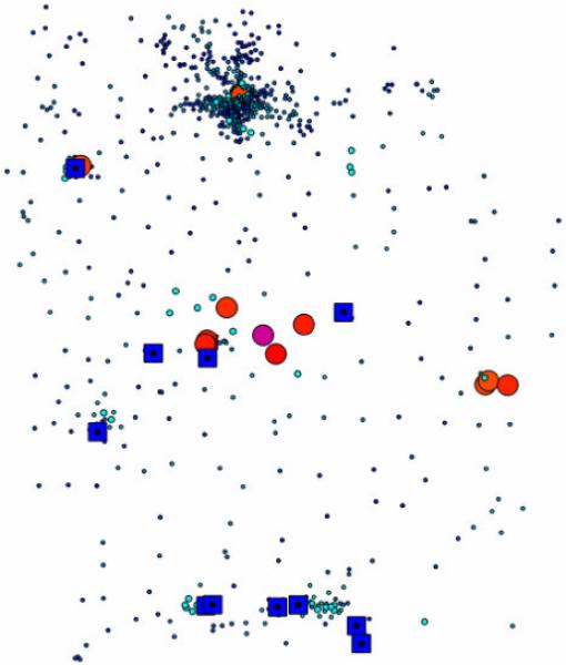
Turnbull’s test for clustering using population radius of 5,000. Circle size and color indicates probability of local clustering: P<0.0001, purple; P<0.001, Red; P<0.01 orange; P>0.01, shades of blue. TCE sites indicated by blue squares.

This illustrates the iterative nature of pattern exploration in which a test may be repeated using different parameter values. Within a formal hypothesis testing framework one can adjust for the multiple testing using the False Discovery Rate (Benjamini 1995; Castro 2006), or show results using adjusted alpha levels such as is accomplished In Figure 5, where only local clusters with p-values <0.001 are colored red.

Question 4: Is there excess leukemia near the Monarch site? This Association question is addressed using a focused method known as the score test. Developed independently by Lawson and Waller, the score test evaluates the pattern of disease frequency around a point focus (Lawson 1989; Waller, Turnbull et al. 1992). The null hypothesis is no clustering relative to the focus, and the alternative hypothesis is that risk increases as one gets closer to the focus. Each region is scored for the difference between observed and expected disease counts, weighted by degree of exposure (proximity) to the focus. The score test is highly significant for the Monarch site (P<0.001) and the alternative hypothesis of increased leukemia risk as distance to the Monarch site decreases is accepted. But is the shape of this risk surface linear, or does it have areas where risk changes rapidly over small distances? This is explored in Question 5.

Question 5: Where are zones of rapid change in leukemia incidence? This Change question is addressed using boundary detection. Methods for delineating local boundaries were originally proposed by Womble and are based on the gradient magnitude of spatial response surfaces (Womble 1951). Locations where variable values change rapidly (e.g. gradients are high) are more likely to be part of a boundary. The local boundaries in leukemia incidence are shown in Figure 6. Using subgraph statistics (Oden 1993; Fortin 1994), these boundaries are found to be significantly longer than expected under the null hypothesis that leukemia incidence occurred at random throughout the study area. But are these boundaries in leukemia associated with the locations of the hazardous waste sites?

Figure 6.

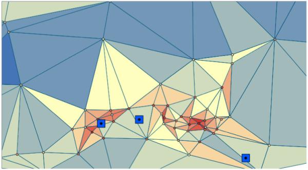
Local zones of rapid change in leukemia incidence found using the Womble method. Reds indicate higher rates of change (derivatives of the leukemia incidence spatial response surface) on the Delaunay network connecting the sampling locations (cenus unit centroids). The TCE sites are shown as blue squares, and are, from left to right, IBM Endicott, Monarch and Singer. Whether or boundaries in leukemia incidence are geographically associated with the locations of the TCE sites is evaluated using boundary overlap statistics (see text).

Question 6: Are zones of rapid change in leukemia incidence associated with hazardous waste sites? This association question is addressed using boundary overlap. Overlap statistics examine whether boundaries in two or more variables coincide, or overlap, to a significant extent (Jacquez 1995). They also can be used to explore whether boundaries are proximate to geographic features such as power lines, rivers, and hazardous waste sites. This approach to overlap analysis is globa1 and is not sensitive to local pockets of association between boundary locations. One of its salient advantages is its ability to evaluate associations between data of different formats, and for which the number of observations vary and are taken at different locations (Hall and Maruca 2001; Hall 2008). Overlap analysis did not find a statistically significant association between the Womble boundaries and the locations of the hazardous waste sites as shown in Figure 6.). This indicates that elevated risk near the TCE sites does not have substantial inflection points (e.g. changes in slope that would correspond to an elevated 2^nd derivative or boundary) as distance from the TCE sites increases. Since this is a global test, it also is possible that pockets of local association are being missed.

Recall our earlier partitioning of leukemia incidence found ~0.86 and ~1.31 cases/1000 population near the Monarch site, which is not excessive given the distribution of incidence in the data set. The overall picture after evaluating these 6 value, change and association questions is that, while incidence indeed increases as distance to the Monarch site decreases, the overall incidence in the direct vicinity of the site is well within the distribution of leukemia incidence observed over the study area.

10. Discussion

This example illustrates how boundary analysis may be used within the framework of Value, Change, and Association questions to yield new insights, extract information, increase knowledge and generate hypotheses regarding the origins and correlates of spatial pattern. Each of the concepts presented has direct extension to the space-time domain, and the application of these techniques to space-time data is an important research direction, as discussed below.

Automated pattern recognition

As the stream of geotemporally referenced data increases we will need automated pattern recognition techniques for assessing how unusual patterns are relative to some expectation (e.g. null model), and for determining whether an observed pattern or set of patterns is associated with (matches) some other pattern. Automation of these techniques will enable systematic evaluation of the burgeoning stream of space-time data. One example of this is the automated detection of patches of disturbed soils from remotely sensed imagery in order to detect mines and the passing of vehicles and small units (Goovaerts, Jacquez et al. 2005). The increasing availability of environmental data from the Sensorweb, sensor networks, and remote imaging technologies, coupled with data streams from over the counter and pharmacy purchases makes possible near real-time surveillance of population as well as individual-level exposures. When working with health data the identification of disease outbreaks using syndromic and health surveillance techniques for analyzing data streams from pharmacies, clinics and hospitals is an important research problem (Dembek, Carley et al. 2005; Kaufmann, Pesik et al. 2005; Lawson, Fitzhugh et al. 2005; Ritzwoller, Kleinman et al. 2005; Berger, Shiau et al. 2006; Cooper, Verlander et al. 2006; Hope, Durrheim et al. 2006).

Neutral models for statistical pattern recognition in human health

Null models play a critical role in statistical pattern recognition, where they specify the “background” against which spatial pattern is evaluated. Most pattern recognition tests used in spatial epidemiology account for heterogeneity in population size, with the local Moran statistic being a notable exception that does not account for impacts of heterogeneous population sizes on the test statistic. Some practitioners advocate the application of empirical Bayesian smoothing to account for rate instability, but this introduces spurious autocorrelation and results in false positives. Almost all socio-demographic and health data evince spatial structure such that nearby areas tend to have similar values. This is expected when artificial spatial partitions (e.g. zipcodes, census boundaries, etc.) are superimposed upon a variable whose value varies continuously through the geographic space. It then is desirable to account for underlying spatial autocorrelation under the null model, rather than employing ‘Complete Spatial Randomness’ (Waller and Gotway 2004). Only when such neutral models are available can we make probabilistic statements regarding observed spatial patterns. For a target map from a real-world system (e.g. map of disease incidence rates), the problem is to generate a set of realizations – simulated maps – with spatial and multivariate characteristics expected under a reasonable null hypothesis. When searching for clusters, such a neutral hypothesis might describe the spatial pattern expected in the absence of clusters – one that will be markedly different from CSR. When searching for boundaries, the neutral hypothesis might describe the spatial pattern expected in the absence of boundaries. A signature (e.g. correlogram, variogram etc.) can be used to quantify spatial pattern under the neutral hypothesis. The problem then is to simulate a set of realizations whose signatures are consistent with this “neutral” signature. Clusters and boundaries are then revealed that are the geographic trace of generating processes above and beyond those giving rise to the neutral signature. Geostatistical approaches to specifying such “neutral models” are proving fruitful, but more research is needed on this important problem (Goovaerts and Jacquez 2004; Goovaerts 2009).

Data fusion

An important and occasionally pernicious problem is that of data fusion – how can we undertake statistical analyses for data that occur in different formats (e.g. vector and raster) and/or at different spatial scales (e.g. census units vs. zipcodes) without introducing spurious autocorrelation via aggregation or kernel smoothing? Techniques such as boundary overlap evaluate association by working with higher order properties of the data (e.g. boundaries) and by incorporating the specifics of the data format (e.g. arrangement of sample locations) into the neutral model. This makes possible statistical analyses that effectively “fuse” diverse formats without compromising the resolution of the data and that do not introduce spurious spatial dependency via spatial filters.

The future

The present state of spatial data analysis follows what has been called the 80-15-5 rule. We spend about 80% of our effort locating and collecting spatial data and reading them into our software systems; 15% of our effort pre-processing (e.g. georectification, atmospheric correction etc) the data, and about 5% of our time actually undertaking spatial analysis and modeling. Perhaps our goal should be to invert this rule, and technological and infrastructure trends seem to be moving in that direction. With internet2, data will be more easily shared and distributed; with the new generation of satellites, high spatial resolution, and hyperspectral imagery are becoming commercially available, providing spatial data that are “clean” and preprocessed. The need for spatial analysis tools in general, and for pattern recognition techniques in particular, is growing. Very fast techniques that can work with massively large, multivariate datasets are needed. One possibility is to leverage the net along the lines of the strategy being used by SETI (Search for extraterrestrial intelligence) and cloud computing to break large pattern recognition problems into logical pieces that can be processed at remote sites.

We will need to be far more effective in sharing our work, data and results. Open spatial analysis software tools and results standards are part of the solution, with the caveat that open software is not well suited to mission-critical applications since quality assurance and software validation may be haphazard or absent in open software.

We need to be able to intelligently specify alternative hypotheses descriptive of the patterns we wish to recognize. As we ask more specific questions, the alternative hypothesis is made more specific. This specialization is accomplished at the cost of a loss of power to detect other departures from the neutral hypothesis. Effective means of balancing this tradeoff are needed. The specification of alternative hypotheses that correspond to reasonable pattern recognition questions while retaining statistical power is thus an important research direction. The resulting “designer pattern recognition techniques” would be an important addition to our spatial and spatio-temporal epidemiology toolbox.

Finally, one of the biggest problems in our data-rich future will be to select between alternative approaches to pattern recognition and data analysis (e.g. distributed agents vs. neural nets vs. statistical pattern detection vs …), which represent tradeoffs between the desire to detect something (but not knowing what that “something” is) and our ability to detect specific patterns based on our prior knowledge of biological and physical systems. It is tempting to look for a magical tool that will detect the “right” pattern, without our having to tell the engine what the “right” pattern is. This extraordinarily difficult problem most likely has no solution. Ultimately the only engine capable of detecting the “right” pattern is one that is guided by careful thought founded on sound science and evidence.