Planar Steering of a Single Ferrofluid Drop by Optimal Minimum Power Dynamic Feedback Control of Four Electromagnets at a Distance

Abstract

Any single permanent or electro magnet will always attract a magnetic fluid. For this reason it is difficult to precisely position and manipulate ferrofluid at a distance from magnets. We develop and experimentally demonstrate optimal (minimum electrical power) 2-dimensional manipulation of a single droplet of ferrofluid by feedback control of 4 external electromagnets. The control algorithm we have developed takes into account, and is explicitly designed for, the nonlinear (fast decay in space, quadratic in magnet strength) nature of how the magnets actuate the ferrofluid, and it also corrects for electro-magnet charging time delays. With this control, we show that dynamic actuation of electro-magnets held outside a domain can be used to position a droplet of ferrofluid to any desired location and steer it along any desired path within that domain – an example of precision control of a ferrofluid by magnets acting at a distance.

2. Introduction

We consider an initial ferrofluid control problem: the precise manipulation of a single drop of ferrofluid by four external electromagnets. Precision control is achieved by feedback: we sense the location of the droplet by a camera and imaging software and then correctly actuate the electromagnets at each time to move it from where it is to closer to where it should be (Figure 1). Repeating this magnetic correction at each time quickly forces the droplet to the desired stationary or moving target and allows us to precisely control its position over time.

Figure 1.

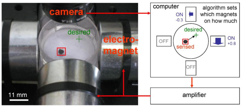
Feedback control of 4 electromagnets can accurately steer a single ferrofluid droplet along any desired path and hold it at any location. Here a camera, computer, amplifier, and the 4 electromagnets are connected in a feedback loop around a petri-dish containing a single droplet of ferrofluid. The camera observes the current location of the droplet; the computer, using the optimal nonlinear control algorithm developed below, computes the electromagnet actuations required to move the droplet from where it is to where it should be; and the amplifier applies the needed voltages to do so. This loop repeats at each time to steer the droplet.

Control design, the mathematical development of the algorithm that determines how to turn on the magnets to create the needed position correction at each time, is challenging. It is recognized that each magnet can only pull the fluid towards it; any single magnet cannot push a magnetic fluid [1, 2]. Further, the available pulling force drops rapidly with the ferrofluid distance from each magnet [3] (see Figure 2 and our derivation in Appendix 3.1 in the supplementary material (www.<fill-in-web-link>)). This makes it difficult to move a ferrofluid droplet left when it is close to the rightmost magnet (the other three magnets must pull it from a long distance, and not over-pull it once it approaches them). Our control algorithm accounts for these difficulties, both for the pulling only nature of each magnet and for the rapid drop off in magnetic force with distance, and it does so in an optimal (minimal electrical power) and smooth fashion. This is done by first finding the set, or manifold, of all electromagnet actuations that will create the desired droplet motion, and then within this manifold picking the minimum power solution. Significant effort has been devoted to insuring that the numerical computations of the optimum are accurate and robust, and a sophisticated nonlinear filter has been integrated into the control to yield smooth magnet actuations that can be implemented experimentally. Our method takes into account electromagnet strength limitations and it corrects for electromagnet dynamics, their charging time lag, by a high-pass temporal filter inserted into the control loop. These innovations provide a scalable control method that can be extended to larger and stronger magnets in the future.

Figure 2.

The magnetic field created by the first magnet and the resulting force on a superparamagnetic particle at any location in the petri dish. The plot is colored by the magnetic field intensity squared on a log scale (log|H²|), and the resulting force directions, according to equation (4) below, are shown by the black arrows at each location. The particle is always attracted to regions of highest magnetic field intensity, i.e. here to the on right magnet. (This, and subsequent theory plots, are shown in non-dimensional variables and magnetic strength units for simplicity of presentation.)

Our interest here is to enable strong magnets to manipulate magnetic particles to deeper targets. As such, we are interested in control algorithms that optimally exploit the capabilities of bigger magnets and that account for their charging time delays. We believe that the algorithms we have designed and demonstrated here can be scaled up to high strength magnets. Compared to our prior work of manipulating single [8, 9] and multiple particles [10] by electric fields and electroosmotic flows [11, 12], which can both pull and push particles, the specific challenges that arise for magnetic control of a single ferrofluid droplet with larger magnets are: 1) The pull only nature of the magnetic actuation. 2) The sharp drop off in magnetic force with distance from the magnet: applying a needed magnetic field when the droplet is far away can easily and dramatically over-pull the droplet as it gets slightly closer to that magnet. 3) The maximum strength constraints of the magnets which provided a hard stop to the amount of control authority available. This makes the minimum electrical power control both reasonable and desirable. 4) The nonlinear cross-coupling between magnets (turning on two magnets at once is not the same as the sum of turning on each magnet individually). A control law based on single magnet actuations will have degraded performance on the diagonals between magnets. Our method works effectively over the entire spatial domain. 5) The related need to switch magnet actuation smoothly in time from one set of magnets to another as the ferrofluid droplet moves through its domain (our control design achieves this). 6) The need to correct for electromagnet coil charging time delays. This last aspect is crucially important for deeper control using larger and stronger magnets that will have longer charging times.

Design and demonstration of control algorithms for minimum power precision control of magnetic particles and fluids is also relevant for magnetofection [13], single particle manipulation (magnetic tweezers) [14–17], lab-on-a-chip systems that include magnetic particles or fluids [18, 19], as well as magnetic drug delivery [20–31]. Magnetofection, the delivery of magnetic particles into cells by an applied magnetic force, could benefit from the approach described here – our technique could be used to position a droplet of magnetic particles above a small region of target cells, and then a magnetic field applied at the bottom could draw the particles into those target cells only. For magnetic particle manipulation, or magnetic tweezers, our methods show how to achieve precision control with the lowest possible electromagnetic powers thus allowing micro-fabricated magnets [16, 19, 32–36], that have a practical limit on how big a magnetic field they can produce, to be placed further apart and to control magnetic particles over a larger spatial domain. Since magnetic tweezing forces scale with particle volume [35, 37], minimum power control should allow more effective manipulation of smaller objects since it will enable available magnets to create manipulation forces more efficiently. Our control results could also benefit dielectrophoresis [38–40] lab-on-a-chip microfluidic applications. DEP and magnetic actuation share the same governing equations for the force on the actuated object (replace the magnetic field H⃑ in equation by the electric field E⃑). Thus the mathematics presented here applies equally to DEP control. Our optimal algorithm could allow each standard 4-electrode DEP pad to steer a single object, with minimum electrical power.

Past work in control of magnetic particles and magnetizable objects has included magnetically assisted surgical procedures, MRI control of ferromagnetic cores and implantable robots, ferrofluid droplet levitation, magnetic tweezers, and nanoparticle magnetic drug delivery in animal and human studies. Methods to manipulate a rigid implanted permanent magnet through the brain with a view to guiding the delivery of hyperthermia to brain tumors are presented in [41] and [42]. Here a point-wise optimization is stated for the magnetic force on the implant and example numerical solutions are shown which display jumps and singularities similar to the ones we had to overcome in this work. Based on market opportunities, the focus of this group changed to magnetically assisted cardiovascular surgical procedures and led to formation of the company Stereotaxis (www.stereotaxis.com/). This company now uses magnetic control to guide catheters, endoscopes, and other tools with magnetic tips for precision treatment of cardiac arrhythmias and other cardiovascular interventions. Stereotaxis catheter control algorithms are not disclosed in detail but are noted briefly in published patents [43–48]. Control of magnetizable devices and ferromagnetic cores using an MRI machine as the actuator are presented by Martel et al [49–51] who also discusses manipulation of implantable magnetic robots [52–54] and magnetic guidance of swimming magnetotactic bacteria [55, 56].

In terms of feedback control of microscopic and nanoscopic magnetizable objects, in [57] a ferrofluid is levitated by feedback control of a single upright electromagnet. Here the droplet of nanoparticles is passively attracted to the electromagnets vertical axis and active feedback is used to modulate the strength of the magnet to stabilize the drop up and down against gravity and disturbances. Two and three dimensional control of magnetic particles in microscopic devices (magnetic tweezers) is described in [14–17, 34, 37] including magnet design and feedback control methods that enable impressively precise and sensitive capabilities for manipulating magnetic microscopic objects [35, 58]. Finally, prior work in magnetic manipulation of therapeutic ferromagnetic nanoparticles (magnetic drug delivery) has progressed to animal and human clinical trials [20, 21, 27, 31, 59]. Magnetic manipulation here is currently limited to static magnets, either held externally [60–65] or implanted [66–71] – as yet there is no active feedback control in this arena.

Compared to prior work, our research here is focused on optimal control for minimum power smooth and deep manipulation of a ferrofluid, with a view towards enabling feedback control of magnetic drug delivery to reach deeper tumors in the long term (see also [4, 5, 7]). To this end, we have addressed the next major step: we have developed and experimentally demonstrated a novel and sophisticated optimal control algorithm to effectively manipulate a single ferrofluid droplet by feedback control. This algorithm was explicitly designed to address the highly nonlinear and cross-coupled nature of dynamic magnetic actuation and to best exploit available electro-magnetic forces.

3. Theory and Modeling

Magnetic fields are described by Maxwell’s equations [72]. In our case, we are changing magnetic fields slowly (compared to radio frequencies) thus the magneto-static equations are appropriate. These are

$$\nabla \times \stackrel{\rightharpoonup }{H}=\stackrel{\rightharpoonup }{j}$$ (1)

$$\nabla ·\stackrel{\rightharpoonup }{B}=0$$ (2)

$$\stackrel{\rightharpoonup }{B}={\mu }_o(\stackrel{\rightharpoonup }{H}+\stackrel{\rightharpoonup }{M})={\mu }_o(\stackrel{\rightharpoonup }{H}+\chi \stackrel{\rightharpoonup }{H}),$$ (3)

where B⃑ is the magnetic field [in Tesla], H⃗ is the magnetic intensity [Amperes/meter], j⃗ is the current density [A/m²], M⃗ is the material magnetization [A/m], χ is the magnetic susceptibility, and μ_o = 4π × 10⁻⁷ N/A² is the permeability of a vacuum. These equations hold true in vacuum and in materials (in air and liquid), for permanent magnets (magnetization M⃗ ≠ 0 ) and for electromagnets (current j⃗ ≠ 0 ). For our simple petri dish surrounded by four electromagnets configuration these equations can be readily solved using MATLAB.

The force on a single superparamagnetic particle is then [7, 26, 73, 74]

$${\stackrel{\rightharpoonup }{F}}_M=\frac{2\pi a^3}{3}·\frac{{\mu }_0\chi }{1+\chi /3}\nabla {\left|\right|\overrightarrow{H}\left|\right|}^2=\frac{4\pi a^3}{3}·\frac{{\mu }_0\chi }{1+\chi /3}{\left(\frac{\partial \overrightarrow{H}}{\partial \overrightarrow{x}}\right)}^T\overrightarrow{H},$$ (4)

where a is the radius of the particle [m], ∇ is the gradient operator [with units 1/m], and ∂H⃑/∂x⃗ is the Jacobian matrix of H⃑ with respect to the position vector x⃗ = (x, y, z). The first relation states that the force on a single particle is proportional to the gradient of the magnetic field intensity squared – i.e. a superparamagnetic particle will always experience a force from low to high applied magnetic field; it will be attracted to any single on magnet regardless of its polarity. The second relation, which is obtained by applying the chain rule to the first one, is more common in the literature and clearly shows that a spatially varying magnetic field (∂H⃑/∂x⃑ ≠ 0 ) is required to create a magnetic force.

If the applied magnetic field is sufficient to magnetically saturate the particle, then (∂H⃑/∂x⃑)^T H⃗ in equation (4) is modified to (∂H⃑/∂x⃑)^T M⃗_sat where M⃑_sat is the saturated magnetization of the particle. Since M⃑_sat lines up with H⃑, this does not change the direction of the force, only its size. In our case, the applied magnetic field never reaches the saturation limit of our particles and so equation (4) is correct as stated for any single magnetic particle.

When a magnetic force is applied, a single particle will accelerate in the direction of that force until it sees an equal and opposite fluid (Stokes) drag force. Since the Stokes force is [75–77]

$${\stackrel{\rightharpoonup }{F}}_S=-6\pi a\eta \stackrel{\rightharpoonup }{v},$$ (5)

where v⃑ is the velocity of the particle relative to the fluid. Our nano-particles come suspended in a solution of deionized water. During experiments, we place them on top of a layer of high viscosity mineral oil (to keep the particles suspended and limit particle interactions with the bottom of the petri dish although the ferrofluid does still sink slowly and eventually does touch the petri dish surface). Thus, for us, the relevant surrounding fluid is the mineral oil and it has a viscosity of η = 0.0576 kg/(m s). Now, setting equation (5) equal to equation (4) and solving for the velocity, we get

$${\stackrel{\rightharpoonup }{v}}_{ss}=\frac{a^2}{9\eta }\frac{{\mu }_0\chi }{1+\chi /3}\nabla {\left|\right|\overrightarrow{H}\left|\right|}^2=k\nabla {\left|\right|\overrightarrow{H}\left|\right|}^2,$$ (6)

where k = a²μ₀χ/9η (1χ/3) is the magnetic drift coefficient (k ≈ 1.6 × 10^{− 20} m⁴/A² s for our 100 nm diameter particles). This steady state velocity is achieved very quickly. For our particles it is predicted to be achieved in nanoseconds (the time constant is computed from Newton’s second law by comparing the nanoparticle mass times acceleration versus the velocity dependent Stokes drag force).

We manipulate a single droplet of ferrofluid, which is composed of very many superparamagnetic nano-particles held together by surface tension and magnetic interactions. The net force on the droplet, and hence its resulting velocity, is still in the direction of ∇ ||H⃗||² as in equations (4) and (6). The issue now is the magnitude of that velocity due to particle-to-particle interactions. Analogously to equation (6), we define k′ as the magnetic drift coefficient for the entire ferro-fluid droplet

$${\stackrel{\rightharpoonup }{v}}_{\mathit{droplet}\_ss}=k^{\prime }\nabla {\left|\right|\overrightarrow{H}\left|\right|}^2.$$ (7)

To quantify k′ we measured droplet velocities under the action of a single magnet for two droplet volumes of 5 and 7.5 μL and compared them to theoretical predictions (see supplementary material Appendix 3.1 (www.<fill-in-web-link>)). The predicted motion best matched the observed motion, for the majority of the droplets trajectory, when k′ ≈ 3.5 × 10⁻¹³ m⁴/A² s and k′ ≈ 4.2 × 10⁻¹³ m⁴/A² s for the two droplet sizes respectively. However, the speed of the motion was under-predicted at the end of the trajectory when the droplet quickly snapped to the edge of the petri dish within the high-field region of the turned on external magnet (Figure SM-3 in the supplementary material appendix (www.<fill-in-web-link>)).

Four scenarios were considered to understand and qualitatively explain the difference between the magnetic drift coefficient predicted for a single particle and that inferred for the ferrofluid droplet: 1) the motion of a single nanoparticle, 2) the motion of a chain of particles held together by magnetic particle-to-particle interactions, 3) the motion of an agglomerate of particles held together by magnetic particle-to-particle and chain-to-chain interactions, and 4) the motion of a rigid ferromagnetic bead the size of the droplet (corresponding to the case where all the particles in the droplet are held together and all act as one mass). Overall, the third option best explained the observed k′ values. Options 1 and 4 dramatically under-predicted and modestly over-predicted k′ respectively. The force on single chains of particles (second option), including a chain of the entire length of the droplet, was also not enough to account for the measured k′ values. Only the third option could explain the measurements and was consistent with prior studies on particle-to-particle interactions which show that particles can form chains and superstructures that dramatically increase the net magnetic force compared to the net viscous drag [78–82]. This explanation is also compatible with our finding that the magnetic drift coefficient varies and is greatest when the droplet is in the high field region near the on magnet: the higher magnetic field increases chaining and superstructures.

We note that our control performance is insensitive to the value of k′ – it continues to work even if we do not know k′ accurately and do not account for its variation with the local magnetic field strength. This is because the control always applies a velocity to move the droplet from where it is towards where it should be – it only needs to set the direction correctly, the magnitude of the velocity is not critically important since another correction will occur at the next time step. Further, the variation in k′ is only appreciable at the edges of the petri dish closest to the external magnets; k′ is close to constant for the majority of the petri dish interior.

Based on the above, we now state the motion of the droplet as a function of the actuation of the four magnets – this is information we need to know in order to design the magnets control law. Let H⃗₁(x, y), H⃗₂(x, y), H⃗₃(x, y), and H⃗₄(x, y) be the magnetic fields in the xy plane, across the petri dish, when each magnet is turned on with a 1 Ampere current. The first magnetic field H⃗₁ (x, y) is shown in Figure 2 as computed by MATLAB, the other three H⃗_k’s are 90 degree rotations of H⃗₁. Let u₁, u₂, u₃ and u₄ be the instantaneous electrical current in each of the four magnets. Then, by the linearity of the magneto-static equations (1) to (3), the time-varying magnetic field that we apply is given by

$$\stackrel{\rightharpoonup }{H}(x,y,t)=u_1(t){\stackrel{\rightharpoonup }{H}}_1(x,y)+u_2(t){\stackrel{\rightharpoonup }{H}}_2(x,y)+u_3(t){\stackrel{\rightharpoonup }{H}}_3(x,y)+u_4(t){\stackrel{\rightharpoonup }{H}}_4(x,y)$$ (8)

In our experiments we checked that this superposition of magnetic fields is valid. The concern was that the magnetic field from one magnet could perturb the core of another magnet. We measured the magnetic field in the petri dish due to the action of one magnet only, due to the action of another magnet only, and when they were both turned on together. We found that the magnetic field due to both magnets was exactly equal to the sum of the magnetic field due to each magnet turned on alone. The explanation for this is that the magnets are sufficiently far apart, and the magnetic fields that they produce fall of sufficiently quickly, that one magnet cannot substantially change the magnetization of the core of another magnet.

In fact, during feedback control, we do not have direct access to the vector of currents $\overrightarrow{u}(t)={\left[\begin{array}{llll}{u}_1(t)\hfill & u_2(t)\hfill & u_3(t)\hfill & u_4(t)\hfill \end{array}\right]}^T$ because we cannot instantaneously charge a magnet to any desired strength. Instead, we control the vector of voltages $\overrightarrow{V}(t)={\left[\begin{array}{llll}{V}_1(t)\hfill & V_2(t)\hfill & V_3(t)\hfill & V_4(t)\hfill \end{array}\right]}^T$.

To first order, the current in each magnet is related to its voltage by simple time delay dynamics [83]. In vector form, this voltage-current relationship for all the magnets is given by

$$\frac{d}{dt}\overrightarrow{u}(t)=-\frac{R}{L}\overrightarrow{u}(t)+\frac{1}{L}\overrightarrow{V}(t),$$ (9)

where R and L are the resistance and inductance of the magnets, respectively. Our control corrects for this time delay by a specially designed nonlinear temporal filter.

Substituting equation (8) into the ferrofluid droplet velocity equation gives the final model for the droplet motion in terms of the applied control

$$\begin{array}{l}\frac{d}{dt}[\begin{array}{ll}x(t)\hfill & y(t)\hfill \end{array}]=k^{\prime }\nabla {\Vert \sum _{i=1}^4{u}_i(t){\overrightarrow{H}}_i(x,y)\Vert }^2=k^{\prime }\sum _{j=1}^4\sum _{i=1}^4{u}_i(t)\left[\nabla ({\overrightarrow{H}}_i(x,y)·{\overrightarrow{H}}_j(x,y))\right]u_j(t)\\ =k^{\prime }\left[\begin{array}{ll}{\overrightarrow{u}}^T(t)P_x(x,y)\overrightarrow{u}(t)\hfill & {\overrightarrow{u}}^T(t)P_y(x,y)\overrightarrow{u}(t)\hfill \end{array}\right]\end{array}$$ (10)

where [x(t) y(t)] is the current location of the droplet in the petri dish, the second equality was achieved by carrying out the square, by multiplying H⃑ = u₁H⃑₁+ u₂H⃑₂+ u₃H⃑₃+ u₄H⃑₄ by itself and then moving the gradient operator into the resulting double summation, and the last equality is a compact matrix representation with subscript T denoting vector transpose and the matrices P_x and P_y defined as

$$\begin{array}{l}{P}_x(x,y)={\left[\partial ({\overrightarrow{H}}_i(x,y)·{\overrightarrow{H}}_j(x,y))/\partial x\right]}_{4\times 4}\\ P_y(x,y)={\left[\partial ({\overrightarrow{H}}_i(x,y)·{\overrightarrow{H}}_j(x,y))/\partial y\right]}_{4\times 4}.\end{array}$$ (11)

All other variables are as defined previously. Together with equation (9) this is the model for droplet motion as a function of the applied control. It is a nonlinear differential equation – the P matrices depend on the droplets location since the magnetic field applied by each magnet varies in space across the petri dish. The dynamics is quadratic in the current control vector u⃑ because the force depends on the gradient of the magnetic field squared. This means the droplets motion depends on both single magnet actuation and on u_iu_j cross terms – the velocity created by turning on two magnets at the same time is not the sum of the velocities created by each magnet alone. Our control is explicitly designed to account for this quadratic nature of the dynamics.

4. Quadratic Model-Based Control

Our control operates by continuously directing the ferrofluid droplet from where it is measured to be towards where it should go (Figure 1). With this approach we can both hold the ferrofluid at a target location (the control continually puts it back) and we can steer the droplet along desired trajectories (the control is always moving the droplet towards its next desired location). At each time we compute a displacement error vector between the droplets desired and measured position d⃑ = x⃑_desired − x⃑_measured and we actuate the four magnets to create a droplet velocity that is along this displacement vector v⃑ = Kd⃑ (the scalar K is our control gain) so that the droplet moves towards its target location. The task of the control algorithm is to decide how to best actuate the four magnets to achieve the needed velocity.

The momentum of the ferrofluid is negligible. This means the droplet has no ability to continue to travel if there is no applied force and it reacts immediately to any newly applied force. Thus the droplets velocity is always in the direction of the magnetic force that we apply (this further means the droplet can execute sharp turns as we show in the results section). The task of the controller to create the needed droplet velocity can be phrased as creating a magnetic force in the right direction at the droplets current location: the two only differ by a constant c, i.e. v⃑ = cF⃑_mag. Although the droplet has no momentum, the electromagnets do. Their actuation cannot be changed sharply (due to coil charging time-constants) and our control takes this into account and compensates for it.

At each moment in time the control has to achieve a desired droplet velocity. This requirement sets two degrees of freedom: the velocity has an x and a y component. But there are four magnets. Thus we have two additional degrees of freedom left over for minimizing control effort. To do this, our control algorithm solves the following problem: it always restricts the four magnet actuations in such a way as to exactly achieve the required velocity vector, it then further optimizes over the remaining two degrees of freedom to choose an actuation that minimizes the consumption of electrical power by the magnets.

The task of achieving a desired droplet velocity v⃗ = (v_x, v_y) can be phrased mathematically in terms of the set of algebraic quadratic equations

$$\begin{array}{l}{k}^{\prime }{\overrightarrow{u}}^T\left[P_x(x,y)\right]\overrightarrow{u}=v_x\\ k^{\prime }{\overrightarrow{u}}^T\left[P_y(x,y)\right]\overrightarrow{u}=v_y.\end{array}$$ (12)

Now, minimizing the electrical power of the magnets is equivalent to minimizing the quadratic cost function

$$J={\left|\right|\overrightarrow{u}\left|\right|}^2={\overrightarrow{u}}^T\overrightarrow{u}.$$ (13)

Therefore, the control problem can be formulated in terms of minimizing (13) subject to the quadratic control constraints (12). Our approach to this optimization problem is to first identify a parametric family of all solutions of (12) (the constraint space), then explicitly express the cost function (13) in terms of the parameters of this family, and finally minimize the cost with respect to the parameters. This converts the original constrained optimization problem to an unconstrained problem. We outline these two steps below and refer to [84] for the details.

At any specific (x, y) droplet location, for each desired velocity v⃑ = (v_x, v_y), the constraint space is a two-dimensional surface in the four-dimensional space of all possible actuations of the magnets – all points u⃑ on this surface create the desired droplet velocity v⃑. Define the vector p⃑ to be the magnetic field at the (x, y) location of the droplet

$$\sum _{j=1}^4{u}_j{\overrightarrow{H}}_j(x,y)=\overrightarrow{p}.$$ (14)

Then the 2-dimensional quadratic constraint of equation (12) can be broken up into two equivalent linear constraints given by equation (14) and the next equation

$$2k^{\prime }\sum _{j=1}^4{u}_j\nabla ({\overrightarrow{p}}^T{\overrightarrow{H}}_j(x,y))=\overrightarrow{v}.$$ (15)

We note that (14) and (15) represent a set of two linear 2-dimensional equations (4 equations total) for u⃗ and p⃑ (for 6 unknowns) instead of one quadratic 2-dimensional equation for u⃑ alone (2 equations for 4 unknowns). The advantage of the second formulation is that it is linear in u⃑ (u_j appears only once in equations (14) and (15), u⃑ appears twice in each equation in (12)). If we choose a specific magnetic field direction, i.e. if we choose a p⃑, then we are left with 4 equations for the 4 actuation variables (u₁, u₂, u₃, u₄). For any p⃑, we can easily solve for u⃑ in terms of p⃑ by a linear inversion. The end results is that the magnetic field itself, at the droplets location, now parameterizes the choice of all possible magnet actuation currents via

$$\overrightarrow{u}={\left[\begin{array}{cccc}\hfill {\overrightarrow{H}}_1(x,y)\hfill & \hfill {\overrightarrow{H}}_2(x,y)\hfill & \hfill {\overrightarrow{H}}_3(x,y)\hfill & \hfill {\overrightarrow{H}}_4(x,y)\hfill \\ \hfill \nabla ({\overrightarrow{p}}^T{\overrightarrow{H}}_1(x,y))\hfill & \hfill \nabla ({\overrightarrow{p}}^T{\overrightarrow{H}}_2(x,y))\hfill & \hfill \nabla ({\overrightarrow{p}}^T{\overrightarrow{H}}_3(x,y))\hfill & \hfill \nabla ({\overrightarrow{p}}^T{\overrightarrow{H}}_4(x,y))\hfill \end{array}\right]}^{-1}\left[\begin{array}{c}\overrightarrow{p}\\ \overrightarrow{v}/2k^{\prime }\end{array}\right]=\overrightarrow{g}(\overrightarrow{p})$$ (16)

that will achieve the desired droplet velocity v⃑. Now we have exactly satisfied the velocity constraint and can search simply over the magnetic field direction p⃗ to find the minimum power control. (Remember that the magnetic field direction p⃑ is not the direction of the applied magnetic force F⃑_mag or, equivalently, the created droplet velocity v⃑. The magnetic force is given by equation (4) and must be in the direction of the desired droplet velocity, the magnetic field is the remaining free parameter over which we now search to find the minimum electrical power control u⃑^*. This split of the problem into a force and field portion is both physically satisfying and yields a well conditioned optimization problem that can be solved cleanly.)

Now, the electrical power cost function J= u⃑^T u⃑ = g⃗^T (p⃗) g⃗(p⃗) must be minimized over p⃗. This optimization problem is easier to solve using polar coordinates p⃗= ρ [cosφ sinφ] for the magnetic field direction. We perform the optimization in two steps: we first minimize J with respect to ρ with φ fixed and we then minimize with respect to φ. The explicit form of u⃑ = g⃗(p⃗) written in equation (16) allows for a closed form solution for the first step, while the second step requires a numerical optimization algorithm. This gives the final optimal control u⃑^*.

The nature of our resulting optimal control algorithm is illustrated in Figure 3 and Figure 4. It minimizes the amount of control effort used and explicitly accounts for the nonlinear nature of the magnetic force. The parameters used for generating these graphs are those of our experimental test-bed. Figure 3 is for a simple case where we wish to move a magnetic droplet along the x-axis from left to right with velocity v⃗ = (1,0). It shows the magnetic potential energy U= −||H⃑||² created in the petri-dish as the drop moves through its x = −0.7, −0.2, +0.2 and +0.7 locations along the horizontal axis (y= 0 ) with unit speed. The magnetic actuations (electrical currents) of each of the four magnets is also displayed (the sign denotes the polarity of the current, positive is clockwise). Notice how the actuation switches from the top and bottom magnets to mainly the right magnet as the droplet is moved from left to right. This is because when the droplet is far away from the right magnet it can be actuated to the right with lower current by using the closer top and bottom magnets.

Figure 3.

Magnetic energy and magnet actuation for control of a ferrofluid droplet from left to right. Each panel is for a different (x,y) droplet location (the black dot). The black arrow is the direction of the desired (and thus applied) magnetic force, the color is the magnetic potential which is equal to minus the magnetic field intensity squared (on a logarithmic scale), and the text inside each magnet states the current through that magnet (positive for clockwise current, negative for counter-clockwise).

Figure 4.

Elements of the optimal control vector u⃑ at different ferrofluid locations in the control region to attain the velocity direction shown at the top left of each panel with minimum electrical power. At each location, the length of each of the lines is proportional to the current to be applied to that magnet, the color (blue or red) corresponds to the sign of the current to be used. Four different directions for the desired velocity v⃑ are shown: 0, 15, 30 and 45 degrees with respect to the x-axis. Magnet actuations for the other seven 45 degree velocity direction sectors (each sector is half a quadrant) are symmetric 90° degree rotations and flips of the 4 cases shown.

Figure 3 is for a droplet velocity that is always to the right. In Figure 4 we show how the 4 magnets must be actuated to control the ferrofluid droplet in any desired direction at any location in the petri dish. Each panel is for a different velocity direction (as shown by the small red line in the green circle at the top left of each panel). Inside each panel, for each droplet (x, y) location, the length of each of the four small lines is proportional to the electrical current that should be applied at each of the four magnets to move a droplet at that (x, y) location along the indicated velocity v⃑ using minimum electrical power. The sign of the currents is coded with blue for positive and red for negative. This plot is read as follows: pick the panel that correspond to the velocity direction that is desired, pick the current location of the ferrofluid drop in the petri dish, the 4 little lines at that location show what magnet currents should be applied in each of the 4 magnets (length corresponds to current strength, blue and red represent a negative or positive current) to move the droplet in the desired direction with minimum electrical power.

Figure 4 presented above determines the vector u⃗ of the electrical currents to be applied to the magnets. However, as stated previously, we can only control the vector V⃗ of the voltages of the magnets. The physical relationship between magnet currents u⃗ and voltages V⃗ is governed by the vector differential equation (9), a first order low-pass filter. It suppresses the high frequency temporal contents of the input V⃗ and is characterized by its cut-off frequency ω = R/L. To prevent distorting the desired value of u⃗ we compensate for the low-pass nature of the magnet physics by a linear high-pass filter in the control loop. This high-pass filter is designed in such a manner that its cascade combination with the low-pass magnet physics leads to a flat frequency response. We use the simplest high-pass filter for achieving this goal which has a first order structure with a zero exactly at ω (to cancel the pole of the low-pass filter) and a pole at ω′>ω, where ω′ is the bandwidth of the output of the control algorithm.

The control also includes a second nonlinear filter. As the droplet moves through space, there are jumps in the type of control that is optimal. This is evident even from the simple straight-line motion case of Figure 3 where it is first optimal to use the nearer top and bottom magnets (first 2 panels) until the droplet gets close enough to the right magnet so that its use becomes preferable (last panel). This kind of magnet switching is fundamental and, if there was no magnet charging time delays, the optimal control of Figure 4 would attempt to apply discontinuous currents in time as the droplet moved through space. The magnet lag and linear high pass filter would smooth these out somewhat. Additionally, we have implemented a specially designed nonlinear filter that smoothes the jumps in time but still ensure that the direction of the applied current vector u⃗(t)= [u₁(t) u₂(t) u₃(t) u₄(t)]^T accurately tracks the direction of the desired optimal current vector shown in Figure 4 (mathematical filter details can be found in [84]). Since, as before, it is the direction of the control vector that sets the direction of the ferrofluid droplet motion, which in turn enables accurate correction of droplet position errors, this nonlinear filter enables a smooth control that does not degrade droplet manipulation performance.

5. Experiment

In this section we describe the details of the experimental setup. As shown in Figure 1, there are four major components, the materials (petri dish, ferrofluid, liquid medium), the camera, the control algorithm software and hardware, and the electromagnets.

5.1. Materials Used

We used a commercially available ferrofluid (Chemicell). The ferrofluid contains 8% by volume of 100 nm diameter multi-core particles. Each particle contains a 70–75 nm in diameter starch encapsulated magnetite core that consists of a fused cluster of single-domain crystals. These magnetic particles were chosen for their size and high magnetic susceptibility (χ~72) which allowed them to be actuated at up to 4 cm away from our moderate strength electromagnets. A future experimental platform with strong magnets is currently under construction and will be able to manipulate a ferrofluid at a greater distance from the magnets.

A 1.5 inch (3.8 cm) diameter Petri-dish (Fisher Scientific) was used to contain the ferrofluid. The petri dish was filled with a high viscosity mineral oil (Heavy Viscosity Mineral Oil, CQ Concepts), which served as a suspending medium for the droplet (as done in [85]). We used mineral oil because of its density, viscosity and surface tension properties which caused the ferrofluid (which comes in the form of magnetic particles suspended in DI water) to remain as a single droplet and significantly reduces sticking of the ferrofluid to the petri dish surface.

5.2. Camera and Real-Time Ferrofluid Position Detection Software

The vision system consisted of a lens, camera, external lighting, and in-house imaging software. The camera (Guppy F-033B/C, 1^st Vision) operated at 58 frames-per-second, had 656 by 494 color pixels, and was equiped with a 6 mm lens (1^st Vision Inc.). A 56-LEDs ring light (Microscope Ring Light, AmScope) was mounted above the petri dish, around the camera, to create a shadow-free illumination of the ferrofluid.

The image software was coded in Matlab version 2007b, with a data acquisition toolbox (version 2.11) and an image acquisition toolbox (version 3.0), and ran on a Dell computer (2.4GHz Intel Core2 Duo CPU). It allowed accurate real-time tracking and velocity estimation of the ferrofluid droplet or blob. This was achieved by combining an algorithm that finds all blobs in an image frame and an algorithm that tracks a blob of interest among other visual features. (It is possible for us to track one droplet through a field of many others [10] by using a Kalman tracking filter but this is not necessary for the results presented in this paper.) Each image frame is transferred from the camera to Matlab through a firewire (IEEE 1394) interface. The image is thresholded, filtered, and operated on by an algorithm that finds the center of the ferrofluid droplet. This method finds and tracks the position of the ferrofluid droplet in less than 20 ms and passes that position to the control algorithm. The vision tracking is completely automated and does not require any user input during control operation.

5.3. Control Algorithm Implementation Hardware and Software

Like the vision code, the control algorithm is written in Matlab and runs on the same computer as the droplet image tracking. It finds the optimal control magnet voltage actuation at each time by solving the mathematics described above, and it takes 66.7 milliseconds to do so (hence the feedback loop runs at 15 Hz). This rate can be improved (e.g. by using C or MEX files to do the evaluation) and that will allow faster control of the ferrofluid in the future.

Output from the computer is used to command the four electromagnets. The computer is connected to a digital-to-analog signal converter (DAQ USB-3101, Measurement Computing) which connects to four linear DC servo amplifiers (MSE421, Mclennan). The latter allows us to increase the low current, low voltage control signal (0–20 mA, ± 10 volts) generated by the digital-to-analog signal converter to the higher current, higher voltage (0–1 A, ± 28 volts) output signal required to power the four electromagnets.

5.4. Electromagnets

We used four small, inexpensive, and commercially available electromagnets to achieve the ferrofluid control results in this paper. These electromagnets (E-28-150 Tubular Electromagnet, Solenoidcity, $57.51 each) have a length of 71.4 mm and a diameter of 38.1 mm each. They contain a 14 mm diameter iron core, their internal resistance was measured to be 43Ω, and they operate at 28 volts while drawing 0.651 amperes. The strength of the magnets was unrated by the manufacturer but we measured the magnetic field distribution around these magnets with a 4.3 mm wide Hall probe (DC Magnetometer (Gauss), AlphaLab Inc.) on a square grid in the petri dish (with a placement accuracy of ~ 1 mm) and a field measurement accuracy of ± 2 % (as rated by the manufacturer) and verified that it matched the simulation data shown in Figure 2. We found that these magnets generated a magnetic field of approximately 0.13 Tesla at their faces, 0.20 Tesla at their corners, and ~0.003 Tesla at a distance of 3.7 cm thus yielding a magnetic field of approximately ~0.016 Tesla at the center of the petri dish. During longer experimental runs, the magnets were cooled by rigid foam ice packs (Fisher Scientific) that were packed around them.

6. Results

We tested our magnetic control for a variety of ferrofluid droplet sizes and desired trajectory shapes and speeds. Droplet volumes were varied from 1 to 20 μL, which, under the action of surface tension, correspond to droplet radii of 0.6 mm and 1.7 mm respectively. We also attempted control of a 150 μL droplet (3.3 mm radius) but this droplet was too large to be held together by surface tension during control and it broke apart. Trajectories were varied from the simplest to more complicated. The simplest task was to control the droplet in a straight line from its current to a desired location (to the center and to the outside of the petri dish). We also controlled the droplets in a square and spiral trajectory, and along ‘UMD’ lettering path (for the University of Maryland). Control speeds were varied from 0.033 to 0.11 mm/s.

Experimental results are shown in figures below and in additional figures in the supplementary material (www.<fill-in-web-link>). In each figure the columns from left to right illustrate a straight line, square, and spiral trajectory. Time progresses from top to bottom and each snapshot shows a trace of the droplets motion for all preceding times. The average error between the desired and actual position of the ferrofluid droplet is defined as

$$e_{\mathit{path}}=\frac{1}{T}{\int }_0^T\left|\right|{\overrightarrow{x}}_{\mathit{desired}}(t)-{\overrightarrow{x}}_{\mathit{measured}}(t)\left|\right|dt,$$ (17)

where T is the amount of time it took to traverse the entire path. For each trajectory the average velocity and this quantitative average path error are noted on the bottom of that column. Below we show the easiest (medium droplet, slow motion) and hardest (small droplet, fast motion) two successful cases, as well as a third case that failed – the large droplet that broke up immediately under the applied magnetic actuation. We also show control along a more complicated ‘UMD’ path. The supplementary material provides figures for all the other cases tested (small droplet slow motion, medium droplet fast motion), as well as movies of the droplet behavior for all cases.

For control of the small 1 μL drop, the visible deviation of the ferrofluid from the desired square and spiral paths near the leftmost electromagnet contributes to most of the average positioning error. This deviation occurs in an operating regime where the magnets are being actuated near saturation. It is possible that the asymmetry seen in the path is due to slightly different saturation characteristics between the four magnets, an aspect that has not yet been accounted for in the control design. Controlling the smaller droplet is harder. The medium size 20 μL droplet can be actuated with less force, the magnets have to work less hard, they do not approach saturation, thus there is virtually no deviation even during fast control (see Figure SM-2 in the supplementary material (www.<fill-in-web-link>)).

Beyond a certain ferrofluid droplet size, the current magnetic position control is no longer possible. For a 150 μL droplet, applied magnetic forces exceed the surface tension forces that hold the droplet together and the droplet is broken up into sub-droplets.

To close this results section we demonstrate control of a single ferrofluid droplet along a ‘UMD’ path, for the University of Maryland.

Above we have shown optimal control of a single droplet to 4 cm depth using four medium-strength (0.13 Tesla at their face), small, commercially available and inexpensive magnets. Based on our mathematical analysis above, using scaled-up stronger (2 Tesla), larger (30 cm length, 30 cm coil diameter, 12 cm core diameter) electromagnets, will enable the same control forces on a single drop of ferrofluid at a depth of half a meter. Advanced magnets with optimally matched materials and shaped coils and cores, as presented in [86–88], could enable even stronger and deeper magnetic control forces.

7. Conclusion

This paper is concerned with precisely manipulating a ferrofluid by external magnets at a distance, and it considers the simplest archetypical example problem: control of a single droplet of ferrofluid in the plane by 4 electromagnets. The control algorithm explicitly takes into account the nonlinear pull-only nature of the magnetic actuation, it is designed for both the quadratic dependence of the magnetic force on the actuated strength of each magnet and the sharp drop off of force with distance from each magnet. Control algorithm design is split into two parts. In the first, the set of all magnetic actuations is found that will move the droplet from where it is towards where it should be. In the second, from this set, the minimal electrical energy actuation is chosen and is applied to the magnets at each time. This gives a robust ability to actuate a single ferrofluid droplet between the four magnets, to any location or along any desired path. Successful numerical optimization and experiments results have shown how to address key practical issues of electromagnet charging time-delays, magnet strength constraints, smooth switching between magnets, and the nonlinear dependence of the applied magnetic pull-only force on space and electromagnetic currents.

Figure 5.

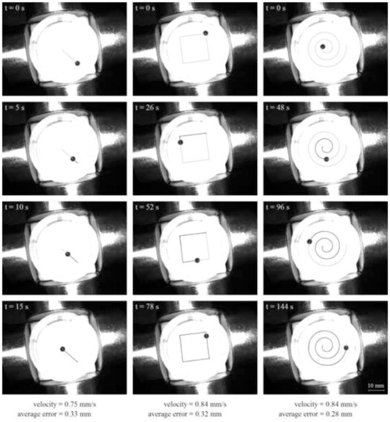
Control of a medium size 20 μL (1.7 mm radius) ferrofluid droplet slowly along a line, square, and spiral path. A quantitative measure of the average error (equation (17)) is noted at the bottom of each column.

Figure 6.

Control of a small 1 μL (0.6 mm radius) ferrofluid droplet faster along a line, square, and spiral path.

Figure 7.

Attempted control of a large 150 μL (3.3 mm radius) ferrofluid droplet. As soon as magnetic control is turned on, the droplet breaks up into multiple smaller droplets. This droplet was too big to control.

Figure 8.

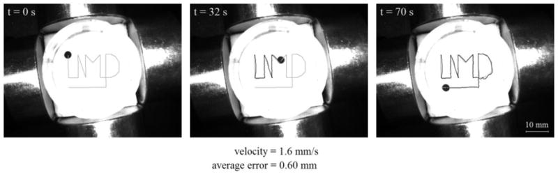
Control of a medium size 20 μL (1.7 mm radius) ferrofluid droplet slowly along a UMD path.

References

- 1.Rosensweig RE. Ferrohydrodynamics. Mineola, NY: Dover Publications, Inc; 1985. [Google Scholar]
- 2.Mikkelsen CI. Department of Micro and Nanotechnology. Technical University of Denmark; Lyngby, Denmark: 2005. Magnetic separation and hydrodynamic interactions in microfluidic systems. [Google Scholar]
- 3.Engel-Herbert R, Hesjedal T. Calculation of the magnetic stray field of a uniaxial magnetic domain. Journal of Applied Physics. 2005;97(7):74504–74505. [Google Scholar]
- 4.Shapiro B, et al. Control to Concentrate Drug-Coated Magnetic Particles to Deep-Tissue Tumors for Targeted Cancer Chemotherapy. 46th IEEE Conference on Decision and Control; New Orleans, LA. 2007. [Google Scholar]
- 5.Shapiro B, et al. Dynamic Control of Magnetic Fields to Focus Drug-Coated Nano-Particles to Deep Tissue Tumors. 7th International Conference on the Scientific and Clinical Applications of Magnetic Carriers; 2008; Vancouver, British Columbia. [Google Scholar]
- 6.Shapiro B, Rutel I, Dormer K. A System to Inject Therapeutically-Coated Magnetic Nano-Particles into the Inner Ear: Design and Initial Validation. Proceedings on the 3rd International Conference on Micro- and Nanosystems (IDETC 200); San Diego, CA: ASME; 2009. [Google Scholar]
- 7.Shapiro B. Towards Dynamic Control of Magnetic Fields to Focus Magnetic Carriers to Targets Deep Inside the Body. Journal of Magnetism and Magnetic Materials. 2009;321(10):1594–1599. doi: 10.1016/j.jmmm.2009.02.094. [DOI] [PMC free article] [PubMed] [Google Scholar]
- 8.Armani M, et al. Using Feedback Control and Micro-Fluidics to Steer Individual Particles. 18th IEEE International Conference on Micro Electro Mechanical Systems; 2005; Miami, Florida. [Google Scholar]
- 9.Armani M, et al. Micro flow control particle tweezers. uTAS; Malmo, Sweden. 2004. [Google Scholar]
- 10.Armani M, et al. Using Feedback Control and Micro-Fluidics to Independently Steer Multiple Particles. Journal of Micro-Electro-Mechanical Systems. 2006;15(4):945–956. [Google Scholar]
- 11.Probstein RF. Physicochemical Hydrodynamics: An Introduction. 2. New York: John Wiley and Sons, Inc; 1994. [Google Scholar]
- 12.Hiemenz PC, Rajagopalan R. Principles of Colloid and Surface Chemistry. 3. New York, Basel, Hong Kong: Marcel Dekker, Inc; 1997. [Google Scholar]
- 13.Schillinger U, et al. Advances in magnetofection—magnetically guided nucleic acid delivery. Journal of Magnetism and Magnetic Materials. 2005;293(1):501–508. [Google Scholar]
- 14.Alenghat FJ, et al. Analysis of Cell Mechanics in Single Vinculin-Deficient Cells Using a Magnetic Tweezer. Biochemical and Biophysical Research Communications. 2000;277(1):93–99. doi: 10.1006/bbrc.2000.3636. [DOI] [PubMed] [Google Scholar]
- 15.Hosu BG, et al. Magnetic tweezers for intracellular applications. Review of Scientific Instruments. 2003;74(9):4158–4163. [Google Scholar]
- 16.Vries AHBd, et al. Micro Magnetic Tweezers for Nanomanipulation Inside Live Cells. Biophysical Journal. 2005;88(3):2137–2144. doi: 10.1529/biophysj.104.052035. [DOI] [PMC free article] [PubMed] [Google Scholar]
- 17.Kanger JS, Subramaniam V, van Driel R. Intracellular manipulation of chromatin using magnetic nanoparticles. Chromosome Research: An International Journal on the Molecular, Supramolecular and Evolutionary Aspects of Chromosome Biology. 2008;16(3):511–522. doi: 10.1007/s10577-008-1239-1. [DOI] [PubMed] [Google Scholar]
- 18.Gijs MAM, Lacharme Fdr, Lehmann U. Microfluidic Applications of Magnetic Particles for Biological Analysis and Catalysis. Chemical Reviews. 2009;110(3):1518–1563. doi: 10.1021/cr9001929. [DOI] [PubMed] [Google Scholar]
- 19.Lehmann U, et al. Two-dimensional magnetic manipulation of microdroplets on a chip as a platform for bioanalytical applications. Sensors and Actuators B: Chemical. 2006;117(2):457–463. [Google Scholar]
- 20.Lubbe AS, et al. Clinical experiences with magnetic drug targeting: A phase I study with 4′-epidoxorubicin in 14 patients with advanced solid tumors. Cancer Research. 1996;56(20):4686–4693. [PubMed] [Google Scholar]
- 21.Lubbe AS, et al. Preclinical experiences with magnetic drug targeting: Tolerance and efficacy. Cancer Research. 1996;56(20):4694–4701. [PubMed] [Google Scholar]
- 22.Ruuge EK, Rusetski AN. Magnetic Fluids as Drug Carriers - Targeted Transport of Drugs by a Magnetic-Field. Journal of Magnetism and Magnetic Materials. 1993;122(1–3):335–339. [Google Scholar]
- 23.Lubbe AS, et al. Physiological aspects in magnetic drug-targeting. Journal of Magnetism and Magnetic Materials. 1999;194(1–3):149–155. [Google Scholar]
- 24.Lubbe AS, Alexiou C, Bergemann C. Clinical applications of magnetic drug targeting. Journal of Surgical Research. 2001;95(2):200–206. doi: 10.1006/jsre.2000.6030. [DOI] [PubMed] [Google Scholar]
- 25.Alexiou C, et al. Magnetic drug targeting - Biodistribution of the magnetic carrier and the chemotherapeutic agent mitoxantrone after locoregional cancer treatment. Journal of Drug Targeting. 2003;11(3):139–149. doi: 10.1080/1061186031000150791. [DOI] [PubMed] [Google Scholar]
- 26.Forbes ZG, et al. An approach to targeted drug delivery based on uniform magnetic fields. IEEE Transactions on Magnetics. 2003;39(5):3372–3377. [Google Scholar]
- 27.Lemke AJ, et al. MRI after magnetic drug targeting in patients with advanced solid malignant tumors. European Radiology. 2004;14(11):1949–1955. doi: 10.1007/s00330-004-2445-7. [DOI] [PubMed] [Google Scholar]
- 28.Simon C. Magnetic drug targeting. New paths for the local concentration of drugs for head and neck cancer. HNO. 2005;53(7):600–601. doi: 10.1007/s00106-005-1278-2. [DOI] [PubMed] [Google Scholar]
- 29.Alexiou C, et al. Distribution of mitoxantrone after magnetic drug targeting: Fluorescence microscopic investigations on VX2 squamous cell carcinoma cells. Zeitschrift Fur Physikalische Chemie-International Journal of Research in Physical Chemistry & Chemical Physics. 2006;220(2):235–240. [Google Scholar]
- 30.Xiong P, et al. Theoretical research of magnetic drug targeting guided by an outside magnetic field. Acta Physica Sinica. 2006;55(8):4383–4387. [Google Scholar]
- 31.Polyak B, Friedman G. Magnetic targeting for site-specific drug delivery: applications and clinical potential. Expert Opinion on Drug Delivery. 2009;6(1):53–70. doi: 10.1517/17425240802662795. [DOI] [PubMed] [Google Scholar]
- 32.Beyzavi A, Nguyen NT. Programmable two-dimensional actuation of ferrofluid droplet using planar microcoils. Journal of Micromechanics and Microengineering. 20(1):015018–015018. [Google Scholar]
- 33.Ramadan Q, et al. Microcoils for transport of magnetic beads. Applied Physics Letters. 2006;88(3):032501–3. [Google Scholar]
- 34.Amblard F, et al. A magnetic manipulator for studying local rheology and micromechanical properties of biological systems. Review of Scientific Instruments. 1996;67(3):818–827. [Google Scholar]
- 35.Gosse C. Magnetic Tweezers: Micromanipulation and Force Measurement at the Molecular Level. Biophysical Journal. 2002;82(6):3314–3329. doi: 10.1016/S0006-3495(02)75672-5. [DOI] [PMC free article] [PubMed] [Google Scholar]
- 36.Fisher JK, et al. Thin-foil magnetic force system for high-numerical-aperture microscopy. Review of Scientific Instruments. 2006;77(2):023702–023702. doi: 10.1063/1.2166509. [DOI] [PMC free article] [PubMed] [Google Scholar]
- 37.Neuman KC, Nagy A. Single-molecule force spectroscopy: optical tweezers, magnetic tweezers and atomic force microscopy. Nat Meth. 2008;5(6):491–505. doi: 10.1038/nmeth.1218. [DOI] [PMC free article] [PubMed] [Google Scholar]
- 38.Pohl HA. Dielectrophoresis: the behavior of neutral matter in nonuniform electric fields. Cambridge University Press; Cambridge: 1978. [Google Scholar]
- 39.Lapizco-Encinas BH, Rito-Palomares M. Dielectrophoresis for the manipulation of nanobioparticles. ELECTROPHORESIS. 2007;28(24):4521–4538. doi: 10.1002/elps.200700303. [DOI] [PubMed] [Google Scholar]
- 40.Edwards B, Engheta N, Evoy S. Electric tweezers: Experimental study of positive dielectrophoresis-based positioning and orientation of a nanorod. Journal of Applied Physics. 2007;102:024913. [Google Scholar]
- 41.Meeker DC, et al. Optimal Realization of Arbitrary Forces in a Magnetic Stereotaxis System. IEEE Transactions on Magnetics. 1996;32(2):320–328. [Google Scholar]
- 42.Creighton FM. Department of Physics. University of Virginia; Charlottesville: 1991. Control of Magnetomotive Actuators for an Implanted Object in Brain and Phantom Materials; p. 203. [Google Scholar]
- 43.Howard MA, III, Ritter RC, Grady MS. Video tumor fighting system. USA: 1989. [Google Scholar]
- 44.Eyssa YM. Apparatus and methods for controlling movement of an object through a medium using a magnetic field. 2005. [Google Scholar]
- 45.Ritter RC. Open field system for magnetic surgery. USA: 2001. [Google Scholar]
- 46.Werp PR. Methods and apparatus for magnetically controlling motion direction of a mechanically pushed catheter. 2002. [Google Scholar]
- 47.Bova FJ, Friedman WA. Computer controlled guidance of a biopsy needle. University of Florida; US: 2003. [Google Scholar]
- 48.Ritter RC, Werp PR, Lawson MA. Method and apparatus for rapidly changing a magnetic field produced by electromagnets. Stereotaxis, Inc; (St. Louis, MO): US: 2000. [Google Scholar]
- 49.Martel S, et al. Automatic Navigation of an Untethered Device in the Artery of a Living Animal Using a Conventional Clinical Magnetic Resonance Imaging System. Applied Physics Letters. 2007;90:114105–1. 4. [Google Scholar]
- 50.Mathieu JB, Beaudoin G, Martel S. Method of Propulsion of a Ferromagnetic Core in the Cardivascular System Through Magnetic Gradients Generated by an MRI System. IEEE Transactions on Biomedical Engineering. 2006;53(2):292–299. doi: 10.1109/TBME.2005.862570. [DOI] [PubMed] [Google Scholar]
- 51.Tamaz S, et al. Real-Time MRI-Based Control of a Ferromagnetic Core for Endovascular Navigation. IEEE Transactions on Biomedical Engineering. 2008;55(7):1854–1863. doi: 10.1109/TBME.2008.919720. [DOI] [PubMed] [Google Scholar]
- 52.Yesin KB, Vollmers K, Nelson BJ. Modeling and Control of Untethered Biomicrorobots in a Fluidic Environment Using Electromagnetic Fields. The International Journal of Robotics Research. 2006;25(5–6):527–536. [Google Scholar]
- 53.Yesin KB, Vollmers K, Nelson BJ. Analysis and design of wireless magnetically guided microrobots in body fluids. Robotics and Automation; Proceedings. ICRA ‘04. 2004 IEEE International Conference; 2004.2004. [Google Scholar]
- 54.Mathieu JB, Martel S. In vivo validation of a propulsion method for untethered medical microrobots using a clinical magnetic resonance imaging system. 2007. [Google Scholar]
- 55.Martel S, et al. Flagellated Magnetotactic Bacteria as Controlled MRI-trackable Propulsion and Steering Systems for Medical Nanorobots Operating in the Human Microvasculature. The International Journal of Robotics Research. 2009;28(4):571–582. doi: 10.1177/0278364908100924. [DOI] [PMC free article] [PubMed] [Google Scholar]
- 56.Martel S, Felfoul O, Mohammadi M. Flagellated bacterial nanorobots for medical interventions in the human body. Biomedical Robotics and Biomechatronics; BioRob 2008. 2nd IEEE RAS & EMBS International Conference; 2008.2008. [Google Scholar]
- 57.Potts HE, Barrett RK, Diver DA. Dynamics of freely-suspended drops. Journal of Physics D-Applied Physics. 2001;34(17):2629–2636. [Google Scholar]
- 58.Lipfert J, Hao X, Dekker NH. Quantitative Modeling and Optimization of Magnetic Tweezers. Biophysical Journal. 2009;96(12):5040–5049. doi: 10.1016/j.bpj.2009.03.055. [DOI] [PMC free article] [PubMed] [Google Scholar]
- 59.Wilson MW, et al. Hepatocellular Carcinoma: Regional Therapy with a Magnetic Targeted Carrier Bound to Doxorubicin in a Dual MR Imaging/Conventional Angiography Suite--Initial Experience with Four Patients. Radiology. 2004;230(1):287–293. doi: 10.1148/radiol.2301021493. [DOI] [PubMed] [Google Scholar]
- 60.Widder KJ, et al. Tumor Remission in Yoshida Sarcoma-Bearing Rats by Selective Targeting of Magnetic Albumin Microspheres Containing Doxorubicin. PNAS. 1981;78(1):579–581. doi: 10.1073/pnas.78.1.579. [DOI] [PMC free article] [PubMed] [Google Scholar]
- 61.Hafeli UO, et al. Effective targeting of magnetic radioactive 90Y-microspheres to tumor cells by an externally applied magnetic field. Preliminary in vitro and in vivo results. Nuclear Medicine and Biology. 1995;22(2):147–155. doi: 10.1016/0969-8051(94)00124-3. [DOI] [PubMed] [Google Scholar]
- 62.Goodwin S, et al. Targeting and retention of magnetic targeted carriers (MTCs) enhancing intra-arterial chemotherapy. Journal of Magnetism and Magnetic Materials. 1999;194(1–3):132–139. [Google Scholar]
- 63.Goodwin SC, et al. Single-Dose Toxicity Study of Hepatic Intra-arterial Infusion of Doxorubicin Coupled to a Novel Magnetically Targeted Drug Carrier. Toxicol Sci. 2001;60(1):177–183. doi: 10.1093/toxsci/60.1.177. [DOI] [PubMed] [Google Scholar]
- 64.Kubo T, et al. Targeted delivery of anticancer drugs with intravenously administered magnetic liposomes in osteosarcoma-bearing hamsters. International Journal of Oncology. 2000;17(2):309–315. doi: 10.3892/ijo.17.2.309. [DOI] [PubMed] [Google Scholar]
- 65.Hirao K, et al. Targeted gene delivery to human osteosarcoma cells with magnetic cationic liposomes under a magnetic field. International Journal of Oncology. 2003;22(5):1065–1071. [PubMed] [Google Scholar]
- 66.Ritter JA, Daniel KD, Ebner AD. High gradient magnetic implants for targeted drug delivery. Abstracts of Papers of the American Chemical Society. 2003;225:U991–U992. [Google Scholar]
- 67.Iacoba GH, et al. Magnetizable needles and wires–modeling an efficient way to target magnetic microspheres in vivo. Biorheology. 2004;41:599–612. [PubMed] [Google Scholar]
- 68.Aviles MO, et al. Theoretical analysis of a transdermal ferromagnetic implant for retention of magnetic drug carrier particles. Journal of Magnetism and Magnetic Materials. 2005;293(1):605–615. [Google Scholar]
- 69.Rosengart AJ, et al. Magnetizable implants and functionalized magnetic carriers: A novel approach for noninvasive yet targeted drug delivery. Journal of Magnetism and Magnetic Materials. 2005;293(1):633–638. [Google Scholar]
- 70.Rotariu O, Strachan NJC. Modeling magnetic carrier particle targeting in the tumor microvasculature for cancer treatment. Journal of Magnetism and Magnetic Materials - Proceedings of the Fifth International Conference on Scientific and Clinical Applications of Magnetic Carriers. 2005;293(1):639–646. [Google Scholar]
- 71.Yellen BB, et al. Targeted drug delivery to magnetic implants for therapeutic applications. Journal of Magnetism and Magnetic Materials. 2005;293(1):647–654. [Google Scholar]
- 72.Feynman RP, Leighton RB, Sands M. The Feynman Lectures on Physics. Addison-Wesley Publishing Company; 1964. [Google Scholar]
- 73.Fleisch DA. A student’s guide to Maxwell’s equations. Cambridge, UK; New York: Cambridge University Press; 2008. [Google Scholar]
- 74.Forbes ZG, et al. Validation of high gradient magnetic field based drug delivery to magnetizable implants under flow. IEEE Transactions on Biomedical Engineering. 2008;55(2 Part 1):643–649. doi: 10.1109/TBME.2007.899347. [DOI] [PubMed] [Google Scholar]
- 75.Incropera FP. Fundamentals of heat and mass transfer. Hoboken, NJ: John Wiley; 2007. [Google Scholar]
- 76.Saltzman WM. Drug delivery: engineering principles for drug therapy. New York, NY: Oxford University Press; 2001. [Google Scholar]
- 77.Smith NP, Pullan AJ, Hunter PJ. An anatomically based model of transient coronary blood flow in the heart. SIAM Journal on Applied mathematics. 2001:990–1018. [Google Scholar]
- 78.Odenbach S. Magnetoviscous Effects in Ferrofluids. Springer; 2002. [Google Scholar]
- 79.Zubarev AY, Odenbach S, Fleischer J. Rheological properties of dense ferrofluids. Effect of chain-like aggregates. Journal of magnetism and magnetic materials. 2002;252:241–243. [Google Scholar]
- 80.Wu M, et al. Magnetic field-assisted hydrothermal growth of chain-like nanostructure of magnetite. Chemical Physics Letters. 2005;401(4–6):374–379. [Google Scholar]
- 81.Mendelev VS, Ivanov AO. Ferrofluid aggregation in chains under the influence of a magnetic field. Physical Review E. 2004;70(5):51502. doi: 10.1103/PhysRevE.70.051502. [DOI] [PubMed] [Google Scholar]
- 82.Wang Z, Holm C. Structure and magnetic properties of polydisperse ferrofluids: A molecular dynamics study. Physical Review E. 2003;68(4):41401. doi: 10.1103/PhysRevE.68.041401. [DOI] [PubMed] [Google Scholar]
- 83.Desoer CA, kuh ES. Basic Circuit Theory: Chapters 1 through 10. McGraw-Hill Inc; US: 1969. [Google Scholar]
- 84.Komaee A, Shapiro B. Steering a Ferromagnetic Particle by Magnetic Feedback Control: Algorithm Design and Validation. Submitted to 2010 American Control Conference. [Google Scholar]
- 85.Lehmann U, et al. Two-dimensional magnetic manipulation of microdroplets on a chip as a platform for bioanalytical applications. Sensors and Actuators B: Chemical. 2005;117(2):457–463. [Google Scholar]
- 86.Creighton FM. Optimal Distribution of Magnetic Material for Catheter and Guidewire Cardiology Therapies. Magnetics Conference (INTERMAG 2006); San Diego, CA: IEEE International; 2006. [Google Scholar]
- 87.Choi JS, Yoo J. Design of a Halbach Magnet Array Based on Optimization Techniques. IEEE Transactions on Magnetics. 2008;44(10):2361–2366. [Google Scholar]
- 88.Alexiou C, et al. A High Field Gradient Magnet for Magnetic Drug Targeting. Applied Superconductivity, IEEE Transactions on. 2006;16(2):1527–1530. [Google Scholar]
- 89.Ui TJ, Hussey RG, Roger RP. Stokes drag on a cylinder in axial motion. Physics of Fluids. 1984;27:787. [Google Scholar]
Associated Data
This section collects any data citations, data availability statements, or supplementary materials included in this article.